Abstract
Most populations of Scots pine in Spain are locally adapted to drought, with only a few populations at the southernmost part of the distribution range showing maladaptations to the current climate. Increasing tree heights are predicted for most of the studied populations by the year 2070, under the RCP 8.5 scenario. These results are probably linked to the capacity of this species to acclimatize to new climates. The impact of climate change on tree growth depends on many processes, including the capacity of individuals to respond to changes in the environment. Pines are often locally adapted to their environments, leading to differences among populations. Generally, populations at the margins of the species’ ranges show lower performances in fitness-related traits than core populations. Therefore, under expected changes in climate, populations at the southern part of the species’ ranges could be at a higher risk of maladaptation. Here, we hypothesize that southern Scots pine populations are locally adapted to current climate, and that expected changes in climate may lead to a decrease in tree performance. We used Scots pine tree height growth data from 15-year-old individuals, measured in six common gardens in Spain, where plants from 16 Spanish provenances had been planted. We analyzed tree height growth, accounting for the climate of the planting sites, and the climate of the original population to assess local adaptation, using linear mixed-effect models. We found that: (1) drought drove differences among populations in tree height growth; (2) most populations were locally adapted to drought; (3) tree height was predicted to increase for most of the studied populations by the year 2070 (a concentration of RCP 8.5). Most populations of Scots pine in Spain were locally adapted to drought. This result suggests that marginal populations, despite inhabiting limiting environments, can be adapted to the local current conditions. In addition, the local adaptation and acclimation capacity of populations can help margin populations to keep pace with climate change. Our results highlight the importance of analyzing, case-by-case, populations’ capacities to cope with climate change.
1. Introduction
The impact of climate change on tree growth is complex, because it depends on many biotic and abiotic processes, and hence, it remains difficult to predict. Northern and western European forests may benefit from warmer temperatures, with positive effects on tree growth [1,2,3,4], but at the same time, tree mortality has increased during the last years [5]. Contrarily, southern and eastern European forests can experience reductions in their growth rates as a consequence of more frequent and intense episodes of drought [1,6]. In natural populations, tree growth strongly depends on climate and stand structure, and on processes related to competition and facilitation among individuals. This complexity varies across geographical scales [4,7,8]. Moreover, tree height growth, related to biomass, and thus, to reproduction, is an important component of fitness with moderate heritability [9] that can show population-level differentiation as a result of local adaptation [10,11]. Likewise, tree height growth can express plasticity (i.e., acclimation) as a result of rapid changes in the environment [12,13].
In the past, natural selection driven by climate may have led to differences among populations in fitness-related traits [10,14]. As a result, tree populations show moderate to strong local adaptation, despite having high levels of gene flow [15]. A locally adapted population is expected to reach its optimum performance (i.e., maximum performance) and outperform non-local populations at its local habitat [16]. However, genetic and demographic processes are different across species’ ranges, leading to remarkable differences between the core and margin populations [17]. Generally, populations’ performances are lower in the margin populations than in the core populations, although this pattern is trait-dependent [12,18]. For instance, tree growth generally declines towards the margins of species’ ranges [19,20], although it can be compensated by trade-offs with other fitness related traits [21,22,23]. Among the different processes that influence trait patterns across species’ ranges, genetic adaptation in margin tree populations is particularly important in the context of climate change.
Common garden experiments (provenance tests) offer an ideal framework to evaluate local adaptation [16,24]. The phenotypic data measured in these experimental designs allow one to estimate populations’ responses to different environments (i.e., reaction norms or plastic responses) and the effect that is attributable to genetic processes. Likewise, common gardens can be used to define a locally adapted population when the local population shows a higher level of fitness (measured from fitness-related traits) than the non-local population when measured in its own habitat [16].
Scots pine (Pinus sylvestris L.) is one of the most widely distributed species in the world [25], with a natural range from beyond the Arctic Circle in Scandinavia to southern Spain, and from western Scotland to the Okhotsk Sea in eastern Siberia. In general, Scots pine tree growth is limited by high temperatures found in the southern part of the range and at low elevations [26], cold temperatures at the northern part of the range and at high elevations [26,27], and by the combination of photoperiod and cold hardiness at the northernmost part of the range [28]. The southern range of Scots pine is reached in Spain. Here, Scots pine presents a fragmented distribution, with high genetic differentiation between populations [29,30,31]. The Spanish populations are mostly found in mountainous areas, growing under the influence of continental or Mediterranean climates, which are characterized by dry summers and cold winters inland, and by mild winters in coastal areas [32], respectively. These marginal populations can be more vulnerable as they inhabit less favorable habitats, where water availability becomes the main constraint of forest growth [33], compromising natural regeneration [34]. Recent warming trends in the climate have exacerbated drought stress, and have negatively impacted tree growth, probably due to an increase in respiration rates and a lower carbon uptake [35,36]. However, these studies have overlooked population-level variation with regard to adaptation and acclimation potential. Previous models, including local adaptation and phenotypic plasticity data, predicted a greater habitat suitability for Scots pine in Spain than classic species distribution models, based exclusively on species occurrence [30], suggesting that these processes are crucial for assessing future predictions of tree height across the species range. However, the extent to which southern Scots pine populations are at a high risk of maladaptation under expected climate change is unclear.
Here, we hypothesize that southern Scots pine populations are locally adapted to the current climate, and that expected changes in climate may lead to a decrease in tree performance. To evaluate our hypothesis, we analyze Scots pine tree height growth data as a proxy of fitness [37,38], from 15-year-old individuals that were measured in a network of common gardens planted in Spain, the southern part of the species’ range. This network gathers six planting sites, in which plants of 16 Spanish provenances had been planted. We define the following objectives: (1) we identify the main climatic drivers shaping among-population differentiation and phenotypic plasticity, (2) we assess if local populations outperform non-local populations at their local environments, and (iii) we predict tree height growth, accounting for the genetic effect of the populations and the phenotypic plasticity, in the southern range of the species under future climates, to assess the impact of climate change.
2. Material and Methods
2.1. Phenotypic Data and Common Gardens
We used the tree height growth data of Scots pine (P. sylvestris) from 15-year-old plants measured in six planting sites established in Spain, the southern range of the species (Figure A1). Sixteen genetically distinct Spanish populations [30,31,39] that cover the species distribution in Spain were planted in each planting site (Figure A1). The seeds for population seedlots were collected during the years 1988 and 1989 [39,40]. A seedlot was composed by mixing the seeds collected in natural populations from at least 25 mother trees, with a 50-m separation distance between each individual, to avoid interbreeding [41]. In 1991, two-year-old plantlets originating from the seedlots were planted in the planting sites, following a randomized complete block design, with four blocks and a 16-tree square plot for each population, planted at a 2.5 × 2.5 m spacing.
2.2. Climate Data
We used two sources of gridded climate data for the present and future conditions:
(1) We used the Gonzalo–Jiménez [42] Spanish climatic model—the average climate was calculated for the period between 1961 and 1999—covering Spain at 30 arc sec resolution (~1 × 1 km), to calibrate our models. We used a total of 51 temperature and precipitation-related climate variables to accurately assess the main climatic drivers promoting among-population differentiation and plasticity (Table 1). We named the climatic variables of the planting site and the population origin _s or _p, respectively (e.g., AHM_s and AHM_p for the annual heat-moisture index of the planting site or at the population origin, respectively).

Table 1.
Temperature- and precipitation-related climate variables considered in the present study.
(2) We used the WorldClim climate database [43,44]—the average climate was calculated for the period between 1970 and 2000—at 30 arc sec resolution (~1 × 1 km), to make spatial predictions of tree height growth for the current and future climates. The climate values for the planting sites and population origins for the current climate were represented by the average climate, as calculated for the period 1970–2000. For future climates, we averaged five global circulation models (GISS-E2-R, HadGEM2-AO, IPSL-CM5A-LR, MIROC-ESM, and NorESM1-M) available in WorldClim [44] for the Representation Concentration Pathway (RCP) 8.5 trajectory for the year 2070. RCPs are greenhouse gas concentration (not emissions) trajectories adopted by the IPCC in the last Assessment Report (AR5) [45]. The RCP 8.5 trajectory is the most aggressive trajectory, and it predicts an increase in the mean temperature of between 2.0 °C and 3.7 °C during the 21st century. Hence, using this scenario for our predictions will show the worst expected outcome. The climate values for the planting sites were represented by the average climate predicted for the year 2070, while the climate values for the populations origins were represented by the average climate of the period 1970–2000.
2.3. Selection of Climate Variables
To identify linear and non-linear co-variations between tree height growth and the climate variables, both between the planting sites and at the populations’ origins, we used Pearson and Spearman correlation analyses. Based on the correlation results, we set a cutoff of ρ ≥ |0.5| to select the climate variables for the planting sites, and of ρ ≥ |0.08|, to select the climate variables for the populations’ origins. For further analyses, all climate variables were standardized: i.e., the mean was subtracted from each value and divided by the standard deviation. We selected 29 climate variables for the planting sites, and five variables for the populations. Climate variables for the planting sites included temperature- and precipitation-related variables, while climate variables for the populations were mostly precipitation-related (Table A1 in Appendix A).
2.4. Linear Mixed-Effect Models of Tree Height Growth
We fitted linear mixed-effect models of tree height growth that accounted for both the climate of the planting site and the climate of the population origin [10,12,13]. To build the best supported linear mixed-effect model, we followed two steps:
(1) We fitted a battery of linear mixed-effect models of pairwise combinations between one climate variable of the planting site, and another climate variable of the population origin from the set of previous selected climate variables to find the best combination. These models included the structure of the experimental design in the random part (two random effects, blocks nested into planting sites, and populations), and the linear and quadratic terms; and the linear interaction term of these climate variables in the fixed part [12] (Equation (1)). We selected the model with the lowest Akaike Information Criterion value (AIC) [46].
where Hijk is tree height growth of the ith individual of the jth population in the kth planting site. αs is the set of n parameters associated with the fixed effects of the model, clim_pij is the climate at the population of origin of the ith individual of the jth population; clim_sik is the climate at the planting site of the ith individual in the kth planting site. βs are the random effects. εijk is the residual distribution of the ith individual of the jth population in the kth planting site following a Gaussian distribution.
Hijk = α0 + α1(clim_s)ik + α2(clim_p)ij + α3(clim_s)ik^2 + α4(clim_p)ij^2 +
α5(clim_s)ik × (clim_p)ij + β1(Planting.site/Block) + β2 (Population) + εijk,
α5(clim_s)ik × (clim_p)ij + β1(Planting.site/Block) + β2 (Population) + εijk,
(2) We built the best supported linear mixed-effect model with the best combination of climate variables selected in the previous step. First, the random part remained invariable, and included the experimental design structure described above (Equation (1)). Second, we defined a full model that included the linear and quadratic terms of both the climate at the planting site and the climate at the population origin, and the linear interaction term of both terms. The model selection of the predictor variables in the fixed part was conducted by using a hierarchical backward selection procedure. We used the AIC criteria, following the rule that net increments of lower than two units of AIC associated with the elimination of any parameter in the full model determined the exclusion of the parameter from the final model [47,48]. We started with the selection of the two-variable interaction (round 1) and then tested the quadratic effects of both climate variables (rounds 2 & 3) and so on downwards the main effects of each predictor (round 4). Fixed effects were tested, using the maximum likelihood (ML), and random effects were tested using the restricted maximum-likelihood method (REML). We computed the percentage of variance explained by the fixed effects of the best supported model, MR2, and the percentage of variance explained by the fixed and random effects together, CR2, [49,50]. The goodness-of-fit of the best model was assessed by examining the predicted vs. observed values. We used normal error distribution with an identity link. We used R (version 3.2.3, 10 December 2015) run in the Linux–GNU operating system to perform all of the analyses, and the ‘‘lme4’’ and “lmerTest” packages [50,51].
2.5. Assessment of the Local Adaptation of Tree Height Growth for Spanish Scots Pine Populations under the Current Climate
Using the best supported linear mixed-effect model, we calculated for each population the tree height growth at its local environment (HL), and the optimum tree height growth (HOPT) attainable at the same environment by a non-local population. To calculate HL, we replaced the climatic values of the planting site by those of the population climate of origin (i.e., clim_s = clim_p). The estimation of HOPT was done in two steps. First, we identified the value of the climate of the population origin, providing the optimum tree height growth (CLOPT), using the best supported mixed-effect model. To do that, we calculated the first-order partial derivate of the best supported linear mixed-effect model with respect to the climate variable of the population origin and settled it to zero [14]. Second, we used CLOPT in our best supported mixed-effect model to obtain HOPT.
The amount of local adaptation of tree height growth for each population was then calculated as follows:
LAH = HOPT − HL,
A positive value of LAH indicates that a non-local population would outperform the local one, suggesting that the local population is not locally adapted. Values of LAH that are equal to or close to zero indicate local adaptation. The higher the value of LAH is, the higher the degree of maladaptation is.
We computed the climate lags (CLH) for each population associated with LAH values, to evaluate the climatic causes of maladaptation; i.e., if the local population does not reach the optimum tree height growth, it could be because it is currently living in a drier or warmer climate (negative values of CLH) or in a wetter or cooler climate (positive values of CLH).
CLH = CLOPT − CLL,
2.6. Spatial Predictions of the Local Adaptation of Tree Height Growth for Southern Scots Pine Populations under the Impacts of the Current and Future Climate
We predicted the optimum tree height growth (HOPT) and local tree height growth (HL) at age 15, based on our models. Our predictions were performed across the species’ range in Spain [52]. Then, we estimated LAH as the difference among them. Moreover, we predicted tree height growth by the year 2070 under the RCP 8.5. scenario (HL-FUT) [53]. Differences between HL-FUT and HL, (DFUT-PRES), can inform us about the climate change impact on Scots pine populations. Positive values of DFUT-PRES mean that Scots pine populations will increase the tree height growth, while negative values would indicate a decrease. We used the ‘raster’ package in R for all of the spatial computations.
3. Results
3.1. Linear Mixed-Effect Models of Tree Height Growth
First, from the battery of models fitted, the model with the lowest AIC included the spring precipitation of the planting site, PREC.spr_s, and the summer heat moisture index of the population origin, SHM_p, (Table A2). Second, the best supported linear mixed-effect model contained the linear term of the spring precipitation of the planting site, PREC.spr_s, and the linear and quadratic terms of the summer heat moisture index of the population origin, SHM_p, and the linear interaction between PREC.spr_s and SHM_p (Table 2 and Table 3). The fixed effects of the model explained 62.36% (MR2) of the variance, and 75.14% (CR2) of the variance was explained by the fixed and random effects together. An examination of the residuals indicated that the main assumptions of linear mixed-effect models were met (Figure A2).
Table 2.
Fixed effects selection for the tree height growth model, following a hierarchical backward procedure using AIC [46] (see Section 2.4 for a detailed description). d.f.: degrees of freedom, AIC: Akaike values, ∆AIC: difference in AIC values between alternative models. MR2 is the percentage of the variance explained by the fixed effects of the model. CR2 is the percentage of the variance explained by the fixed and random effects of the model. MR2 and CR2 values are given for the best supported mixed-effect model.
Table 3.
Mean, standard error (SE), t-values and p-values are given for the fixed effects of the tree height growth model in the first panel; and standard deviation (SD) for the random effects are given in the second panel.
The spring precipitation of the planting sites (PREC.spr_s) had a positive effect on tree height growth (Figure 1). The summer heat moisture index (SHM_p) drove the among-population differentiation in the studied populations. Specifically, populations that originated in sites with intermediate values of the summer heat moisture index, SHM, displayed the highest tree height growth, while populations that originated in sites with either high or low values of SHM presented lower tree height growth. This pattern varied across the PREC.spr_s gradient, due to the interaction term between PREC.spr_s and SHM_p (Table 3 and Figure 1).
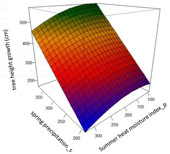
Figure 1.
Predicted tree height growth (cm), based on the best supported linear mixed-effect model across the gradients of spring precipitation of the planting sites, PREC.spr_s, and of the summer heat moisture index of the populations’ origin, SHM_p.
3.2. Assessment of the Local Adaptation of Tree Height Growth for Spanish Scots Pine Populations under the Current Climate
Most of the populations, except two, underperformed at their local environment, as shown by LAH values that were different from zero (Table 4). However, the LAH values were small, and they were specifically below 5 cm in 11 out of the 16 populations tested (Table 4). Most of the populations were currently growing under drier conditions, as we found negative values in climatic lags CLH. This may prevent the optimum tree height growth from being reached. Two out of the 16 populations were growing under wetter conditions, as we found positive values in CLH (Table 4).
Table 4.
Predictions of local tree height growth, HL (cm), and optimum tree height growth, HOPT (cm), for each population, based upon the best supported model.
3.3. Spatial Predictions of the Local Adaptation of Tree Height Growth for Southern Scots Pine Populations under the Impacts of the Current and Future Climate
Most southern Scots pine populations are locally adapted (LAH values close to zero) or slightly maladapted (LAH values of around 5; gray to light-yellow colors in Figure 2) to current climates. Just a few populations of Scots pine at the southernmost part of the distribution presented large values of LAH (yellow to red colors in Figure 2).
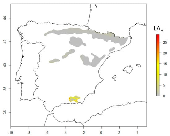
Figure 2.
Local adaptation of tree height growth to current climate for southern Scots pine populations at 15 years-old (LAH, cm) in Spain. LAH provides a measurement of the local adaptation in cm. Zero values indicate local adaptation, the rest of the values denote a lack of local adaptation. Gray to light-yellow colors indicate that the populations are locally or slightly maladapted (LAH ranges between 0 and 5 cm), whilst yellow to red colors indicate populations maladapted to the current climate (LAH > 5 cm).
Our model predicted an increase in tree height growth in year 2070, particularly in the north (Pyrenees), and in high-elevation areas (Figure 3). The model predicted a decrease in tree height growth in the center and in the north-west. Populations at the southernmost part of the distribution were predicted to decrease moderately (Figure 3).
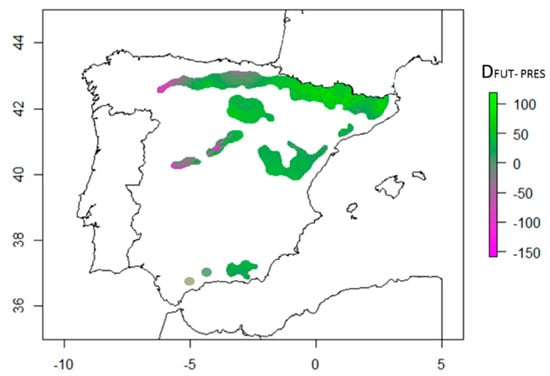
Figure 3.
Differences in tree height growth predictions (DFUT-PRES, cm) between future (year 2070, RCP 8.5.) and tree height growth for current climate conditions. Violet to gray colors indicate a decrease in tree height predicted for 2070, and gray to green colors indicate an increase in the potential tree height growth, as predicted by the model.
4. Discussion
4.1. The Main Climatic Drivers Shaping Among-Population Differentiation and Phenotypic Plasticity Responses of Tree Height Growth
The main climatic driver shaping genetic differentiation among the populations, in terms of tree height growth, was the summer moisture index (SHM_p), a proxy of drought. This result suggests that drought has probably been a selective factor, which is in agreement with previous studies [39,54]. For instance, our model predicted that populations that originated under more stressful conditions, i.e., with higher values of the summer moisture index calculated for the period of years between 1961 and 1999 (Figure 1), would present a slower rate of growth, which is a suggested strategy for increasing drought adaptation by reducing aboveground biomass [39,55]. Other adaptive responses to reduce cavitation risks, induced either by drought or frost stresses, have been described for the same populations. For example, populations from dry sites show large average tracheid lumen diameters, to assure hydraulic conductivity, whilst populations from sites with frequent freeze–thaw events present small tracheid lumen diameters [53]. Also, it has been suggested that southern populations adapt their leaf conductance and stomata control for less transpiration through the needles [54].
Phenotypic plastic responses were driven by spring precipitation (PREC.spr_s). We found a common pattern where tree height growth decreases under drier conditions (Table 3 & Figure 1). This result agrees with the findings of a previous study, where annual precipitation drove phenotypic plastic responses in tree height–diameter allometry for the same species [40]. Now, this study has allowed us to identify that tree height growth is largely driven by the rainfall that falls during the spring season. This could be related to the fact that maximum cambial activity for this species has been described to take place between mid-March and end of August [55], suggesting that Scots pine populations make better use of the rainfall in the early growing season than in the late season (autumn).
Both results highlight that water availability drives the phenotype variations in tree height growth in Scots pine populations, which is consistent with the limiting role that water plays in Mediterranean ecosystems [56].
4.2. Most Southern Scots Pine Populations are Locally Adapted to the Current Climate
The finding of local adaptations for most of the southern Scots pine populations was in agreement with our expectations (Table 4 & Figure 2). One possible explanation could be related to the species’ demographic history. During the last glacial maximum, Scots pine had many refuge areas scattered throughout southern Europe [57,58]. These populations may have adapted to the particular conditions of this part of the range during the postglacial migrations [24,33]. Furthermore, the fragmented distribution of the species in the southern part of the range, and the low levels of gene flow among populations might have favored local adaptation [31]. However, we found maladaptation in the southernmost populations (Figure 2). This result could be explained accordingly by the gene flow asymmetry theory across species’ ranges [14]: maladapted populations might have received alleles from core and northern populations that are pre-adapted to cooler or wetter conditions than those found at the southernmost part of the range, limiting local adaptation [10,14].
Nevertheless, our findings of local adaptation may change if other fitness-related traits were considered. For instance, fitness-related traits can present trade-offs across the species’ ranges [21,23]. Typically, demographic compensation has been found in several marginal populations [21,22,23]. We could expect the same for Scots pine, given that the southernmost Spanish populations show low early recruitment as a consequence of high seedling mortality, low seed production, and high predation rates [56]. Hence, a wider perspective of Scots pine adaptation patterns using other traits than those related with growth is desirable.
4.3. The Importance of Considering Genetic and Plastic Effects for Evaluating Tree Height Growth for Future Climates
Our predictions should be interpreted as the combination of adaptation and plasticity effects in tree height growth. The contribution of genetic effects to explain tree growth variation in our data was lower than that of phenotypic plasticity, although it was of similar magnitude (∆AIC = 28.69 and ∆AIC = 33.94, respectively, Table 1). This result highlights that both adaptations to local conditions and the capacity to adjust to the environment through plastic responses are crucial for understanding the performance of Scots pine populations for future climates.
Future predictions for an average tree, showing an increase in tree height, suggest that plasticity can help with tree acclimation to the new climate, and it can then compensate for the imprint of local adaptation, which is a common characteristic in trees [57]. Our results are partially in agreement with [27], where moderate increases in tree growth for Scots pine populations are predicted in Spain under the RCP 8.5 scenario for 2050, although tree growth does decrease, especially in southern low-elevation sites, in 2070. In the northern and high-elevation areas (Pyrenees), warmer conditions would benefit tree growth by lengthening the growing season, thus increasing net photosynthesis, stomatal conductance, and specific hydraulic conductivity [58]. However, opposite results of tree growth decrease have been reported for this species in Spain [35,59], as lower precipitation regimes combined with higher temperatures would presumably lead to a general pattern of more frequent drought events, higher evapotranspiration, and reduced soil water availability in the future. However, none of these studies have accounted for the plasticity capacity of the species, and this could explain the differences in the forecasts. Moreover, few populations in the north-west and in the central part of the species distribution in Spain have been predicted to decrease in tree height growth. This prediction could be reflected by the sharp decrease in spring precipitation that is expected for year 2070 (RCP 8.5.) in these areas (Figure A3). Our forecast could be related to site characteristics (such as soil depth, nutrient availability, geomorphological features, etc.) that can make water availability difficult.
Finally, caution is needed when interpreting our predictions beyond the year 2070, as we do not know whether plasticity will help with acclimation to new environments in the far future, and evolutionary adaptation may then become necessary. Contrary to our expectations, in terms of the species’ growth, the forecast for southern Scots pine populations is generally favorable. Nonetheless, our results are based on common gardens. In natural populations, other factors, such as above- and below-ground competition, herbivory, management practices, etc., can strongly modify our expectations of Scots pine growth and adaptation to climate change.
5. Conclusions
Most of the populations of Scots pine in Spain were locally adapted to drought. This result suggests that marginal populations, despite inhabiting limiting environments, can become adapted to their current local conditions. In addition, the local adaptation and acclimation capacity of populations can help marginal populations to keep pace with climate change. Our results highlight the importance of analyzing populations’ capacity to cope with climate change, on a case-by-case basis.
Author Contributions
In the present study, the authors contributed to the different sections as follows: Conceptualization, N.V.-P. and M.B.G.; methodology, N.V.-P., N.G.-M. and M.B.G.; formal analysis, N.V.-P.; manuscript writing—original draft preparation N.V.-P., N.G.-M., and M.B.G.; writing—review and editing N.V.-P., S.C.G.-M., R.A., M.B.G.
Funding
This study was funded by: the Spanish Ministry of Economy and Competitiveness, through the following projects VULPINECLIM (MINECO, CGL2013-44553-R), ADAPCON (CGL2011-30182-C02-01), FENOPIN (AGL2012-40151-C03-02), and the following two projects: “Investments for the future” Programme IdEx Bordeaux (reference ANR-10-IDEX-03-02) and the EFPA (Département Ecologie des Forêts, Prairies et milieux Aquatiques) INRA (Institut National de la Recherche Agronomique) Integration Project. NVP was funded by a fellowship FPI-MCI (BES-2009-025151) and a postdoctoral contract associated with the European Project H2020 “Optimising the management and sustainable use of forest genetic resources in Europe” (GenTree; grant agreement No 676876)”. NGM was supported by an AgreenSkills postdoctoral fellowship. The data is part of the Spanish Network of Genetic Trials (GENFORED), and it is publicly available upon request through www.genfored.es.
Acknowledgments
We acknowledge the GENFORED team: F. del Caño, E.D. Barba, F.J. Auñón, and M.R. Chambel—who measured, gathered, and stored the data used in this research article.
Conflicts of Interest
The authors declare no conflict of interest.
Appendix A
Table A1.
Pearson and Spearman correlation coefficients between climate data, at the planting sites and at the population origin, and tree height growth of Scots pine from 15-year-old.
Table A1.
Pearson and Spearman correlation coefficients between climate data, at the planting sites and at the population origin, and tree height growth of Scots pine from 15-year-old.
| Climate at the Planting Site | Climate at the Population Origin | ||||
|---|---|---|---|---|---|
| Variables | Pearson | Spearman | Variables | Pearson | Spearman |
| TMF.jan | −0.565 | −0.384 | TMF.jan | 0.025 | 0.019 |
| TMF.feb | −0.581 | −0.497 | TMF.feb | 0.006 | 0 |
| TMF.mar | −0.62 | −0.554 | TMF.mar | 0.007 | −0.002 |
| TMF.apr | −0.65 | −0.616 | TMF.apr | 0.004 | −0.004 |
| TMF.may | −0.371 | −0.382 | TMF.may | −0.007 | −0.01 |
| TMF.jun | −0.055 | −0.111 | TMF.jun | −0.002 | 0.003 |
| TMF.jul | −0.107 | −0.038 | TMF.jul | −0.016 | −0.025 |
| TMF.ago | −0.171 | 0.009 | TMF.ago | −0.021 | −0.036 |
| TMF.sep | −0.534 | −0.536 | TMF.sep | −0.014 | −0.029 |
| TMF.oct | −0.633 | −0.554 | TMF.oct | 0.005 | −0.009 |
| TMF.nov | −0.636 | −0.594 | TMF.nov | 0.01 | 0.006 |
| TMF.dec | −0.577 | −0.479 | TMF.dec | 0.024 | 0.01 |
| TMC.jan | −0.32 | −0.174 | TMC.jan | −0.017 | −0.031 |
| TMC.feb | −0.478 | −0.47 | TMC.feb | −0.03 | −0.023 |
| TMC.mar | −0.628 | −0.644 | TMC.mar | −0.043 | −0.039 |
| TMC.apr | −0.648 | −0.644 | TMC.apr | −0.034 | −0.037 |
| TMC.may | −0.607 | −0.695 | TMC.may | −0.055 | −0.057 |
| TMC.jun | −0.469 | −0.345 | TMC.jun | −0.055 | −0.064 |
| TMC.jul | −0.494 | −0.478 | TMC.jul | −0.075 | −0.087 |
| TMC.ago | −0.379 | −0.378 | TMC.ago | −0.075 | −0.086 |
| TMC.sep | −0.438 | −0.44 | TMC.sep | −0.077 | −0.086 |
| TMC.oct | −0.443 | −0.521 | TMC.oct | −0.034 | −0.024 |
| TMC.nov | −0.269 | −0.208 | TMC.nov | −0.028 | −0.027 |
| TMC.dec | −0.287 | −0.174 | TMC.dec | −0.016 | −0.014 |
| T.jan | −0.457 | −0.407 | T.jan | 0.003 | 0 |
| T.feb | −0.569 | −0.497 | T.feb | −0.014 | −0.018 |
| T.mar | −0.66 | −0.684 | T.mar | −0.023 | −0.022 |
| T.apr | −0.648 | −0.616 | T.apr | −0.019 | −0.027 |
| T.may | −0.586 | −0.616 | T.may | −0.034 | −0.037 |
| T.jun | −0.337 | −0.345 | T.jun | −0.03 | −0.029 |
| T.jul | −0.358 | −0.282 | T.jul | −0.048 | −0.052 |
| T.ago | −0.311 | −0.378 | T.ago | −0.051 | −0.049 |
| T.sep | −0.492 | −0.378 | T.sep | −0.05 | −0.042 |
| T.oct | −0.534 | −0.521 | T.oct | −0.016 | −0.027 |
| T.nov | −0.466 | −0.521 | T.nov | −0.011 | −0.023 |
| T.dec | −0.426 | −0.407 | T.dec | 0.001 | −0.006 |
| PREC.annl | 0.675 | 0.663 | PREC.ann | 0.073 | 0.105 |
| PREC.win | 0.575 | 0.516 | PREC.win | 0.035 | 0.038 |
| PREC.spr | 0.779 | 0.663 | PREC.spr | 0.073 | 0.088 |
| PREC.sum | 0.609 | 0.497 | PREC.sum | 0.08 | 0.079 |
| PREC.son | 0.611 | 0.487 | PREC.son | 0.079 | 0.107 |
| MT | −0.544 | −0.458 | MT | −0.024 | −0.031 |
| MCMT | −0.262 | −0.282 | MCMT | −0.056 | −0.057 |
| MAXWMT | −0.416 | −0.378 | MAXWMT | −0.072 | −0.083 |
| MCMT | −0.446 | −0.407 | MCMT | 0.01 | 0.007 |
| MINCMT | −0.561 | −0.351 | MINCMT | 0.031 | 0.027 |
| FP | 0.651 | 0.594 | FP | −0.016 | 0.009 |
| DD5 | −0.613 | −0.548 | DD5 | −0.004 | −0.012 |
| TD | 0.282 | 0.33 | TD | −0.103 | −0.107 |
| AHM | −0.611 | −0.663 | AHM | −0.083 | −0.087 |
| SHM | −0.376 | −0.554 | SHM | −0.108 | −0.103 |
T.#, TMC.# and TMF.# mean minimum, maximum and mean average monthly (#) temperatures (°C); PREC.ann means annual precipitation (mm); PREC.win, PREC.spr, PREC.sum, PREC.aut, for winter, spring, summer and autumn, respectively; TM means mean annual temperature (°C); MINCMT means mean of the minimum temperatures from the coldest month (°C); FP means frost period (month); DD5 means degree days-period over 5 °C; TD means continentality; AHM means annual heat moisture index; and SHM means summer heat moisture index.
Table A2.
AIC values from the battery of linear-mixed effect models fitted. Climate variables of the planting sites are specified with _s and climate at the populations’ origin with _p. The best supported model showed the lowest AIC and it is highlighted with bold.
Table A2.
AIC values from the battery of linear-mixed effect models fitted. Climate variables of the planting sites are specified with _s and climate at the populations’ origin with _p. The best supported model showed the lowest AIC and it is highlighted with bold.
| PREC.ann_p | PREC.sum_p | PREC.aut_p | TD_p | SHM_p | |
|---|---|---|---|---|---|
| TMF.jan_s | 49,559.63 | 49,551.74 | 49,554.15 | 49,557.09 | 49,546.44 |
| TMF.feb_s | 49,560.72 | 49,551.38 | 49,555.08 | 49,557.30 | 49,547.21 |
| TMF.mar_s | 49,560.71 | 49,550.99 | 49,555.01 | 49,557.11 | 49,546.92 |
| TMF.apr_s | 49,560.68 | 49,551.40 | 49,555.01 | 49,557.05 | 49,546.58 |
| TMF.sep_s | 49,559.38 | 49,550.93 | 49,554.04 | 49,557.11 | 49,546.46 |
| TMF.ocT_s | 49,560.05 | 49,550.89 | 49,554.45 | 49,556.87 | 49,546.21 |
| TMF.nov_s | 49,560.59 | 49,550.80 | 49,554.90 | 49,557.00 | 49,546.73 |
| TMF.dec_s | 49,558.35 | 49,551.16 | 49,553.06 | 49,556.43 | 49,545.56 |
| TMC.mar_s | 49,559.41 | 49,551.82 | 49,553.99 | 49,556.32 | 49,545.58 |
| TMC.apr_s | 49,560.07 | 49,551.58 | 49,554.50 | 49,556.48 | 49,545.95 |
| TMC.may_s | 49,558.67 | 49,550.63 | 49,553.19 | 49,555.64 | 49,544.68 |
| TMC.ocT_s | 49,560.10 | 49,551.94 | 49,554.42 | 49,557.14 | 49,546.54 |
| T.feb_s | 49,560.11 | 49,551.59 | 49,554.50 | 49,557.14 | 49,546.43 |
| T.mar_s | 49,559.29 | 49,550.86 | 49,553.77 | 49,556.02 | 49,545.26 |
| T.abr_s | 49,560.58 | 49,551.67 | 49,554.94 | 49,556.90 | 49,546.43 |
| T.may_s | 49,559.93 | 49,551.30 | 49,554.34 | 49,556.65 | 49,545.82 |
| T.ocT_s | 49,560.85 | 49,552.14 | 49,555.19 | 49,557.78 | 49,547.12 |
| T.nov_s | 49,560.74 | 49,552.16 | 49,554.99 | 49,557.50 | 49,547.12 |
| PREC.ann_s | 49,556.66 | 49,547.51 | 49,551.56 | 49,554.96 | 49,542.98 |
| PREC.win_s | 49,557.89 | 49,548.82 | 49,553.03 | 49,557.20 | 49,544.34 |
| PREC.spr_s | 49,551.91 | 49,542.89 | 49,546.79 | 49,549.92 | 49,537.76 |
| PREC.sum_s | 49,559.40 | 49,550.01 | 49,553.93 | 49,556.48 | 49,545.86 |
| PREC.aut_s | 49,558.02 | 49,548.82 | 49,552.83 | 49,555.99 | 49,544.56 |
| TM_s | 49,560.08 | 49,551.91 | 49,554.55 | 49,557.53 | 49,546.59 |
| MINCMT_s | 49,559.40 | 49,551.46 | 49,553.88 | 49,556.69 | 49,546.14 |
| FP_s | 49,559.60 | 49550.39 | 49,553.99 | 49,556.29 | 49,545.69 |
| DD5_s | 49,559.15 | 49,550.99 | 49,553.67 | 49,556.52 | 49,545.53 |
| AHM_s | 49,553.34 | 49,546.99 | 49,548.73 | 49,553.97 | 49,541.36 |
| SHM_s | 49,557.06 | 49,551.09 | 49,551.97 | 49,556.55 | 49,545.83 |
T.#, TMC.# and TMF.# mean minimum, maximum and mean average monthly (#) temperatures (°C); PREC.ann means annual precipitation (mm); PREC.win, PREC.spr, PREC.sum, PREC.aut, for winter, spring, summer and autumn, respectively; TM means mean annual temperature (°C); MINCMT means mean of the minimum temperatures from the coldest month (°C); FP means frost period (month); DD5 means degree days-period over 5 °C; TD means continentality; AHM means annual heat moisture index; and SHM means summer heat moisture index.

Figure A1.
Network of provenance common gardens in Spain (GENFORED): Planting sites (green crosses), populations (pink circles). The species distribution range is shown in gray (two isolated populations are represented by “+” in gray).

Figure A2.
Graphical summary of the best supported model for Scots pine populations from 15 year-old. Top line, left to right: plot of observed raw data vs. predicted; plot of observed raw data vs. predicted data; residuals vs. predicted data. Middle line: qq-plot; histogram of residuals values; residuals vs. shm_p (summer heat moisture index). Bottom line: residuals vs. prec.mam_s (spring precipitation); residuals vs. population factor; residuals vs. planting site factor.

Figure A3.
Spring precipitation anomaly between year 2070 (RCP 8.5) and current climate (baseline: average climate calculated for the period 1970–2000).
References
- Lindner, M.; Maroschek, M.; Netherer, S.; Kremer, A.; Barbati, A.; Garcia-Gonzalo, J.; Seidl, R.; Delzon, S.; Corona, P.; Kolström, M.; et al. Climate change impacts, adaptive capacity, and vulnerability of European forest ecosystems. For. Ecol. Manag. 2010, 259, 698–709. [Google Scholar] [CrossRef]
- Pretzsch, H.; Biber, P.; Schütze, G.; Uhl, E.; Rötzer, T. Forest stand growth dynamics in Central Europe have accelerated since 1870. Nat. Commun. 2014, 5, 4967. [Google Scholar] [CrossRef] [PubMed]
- McMahon, S.M.; Parker, G.G.; Miller, D.R. Evidence for a recent increase in forest growth. Proc. Natl. Acad. Sci. USA 2010, 107, 3611–3615. [Google Scholar] [CrossRef] [PubMed]
- Machar, I.; Vlckova, V.; Bucek, A.; Vozenilek, V.; Salek, L.; Jerabkova, L.; Machar, I.; Vlckova, V.; Bucek, A.; Vozenilek, V.; et al. Modelling of Climate Conditions in Forest Vegetation Zones as a Support Tool for Forest Management Strategy in European Beech Dominated Forests. Forests 2017, 8, 82. [Google Scholar] [CrossRef]
- Allen, C.D.; Macalady, A.K.; Chenchouni, H.; Bachelet, D.; McDowell, N.; Vennetier, M.; Kitzberger, T.; Rigling, A.; Breshears, D.D.; Hogg, E.H.; et al. A global overview of drought and heat-induced tree mortality reveals emerging climate change risks for forests. For. Ecol. Manag. 2010, 259, 660–684. [Google Scholar] [CrossRef]
- Lévesque, M.; Siegwolf, R.; Saurer, M.; Eilmann, B.; Rigling, A. Increased water-use efficiency does not lead to enhanced tree growth under xeric and mesic conditions. New Phytol. 2014, 203, 94–109. [Google Scholar] [CrossRef]
- Gómez-Aparicio, L.; García-Valdés, R.; Ruiz-Benito, P.; Zavala, M.A. Disentangling the relative importance of climate, size and competition on tree growth in Iberian forests: Implications for forest management under global change. Glob. Chang. Biol. 2011, 17, 2400–2414. [Google Scholar] [CrossRef]
- Kunstler, G.; Falster, D.; Coomes, D.A.; Hui, F.; Kooyman, R.M.; Laughlin, D.C.; Poorter, L.; Vanderwel, M.; Vieilledent, G.; Wright, S.J.; et al. Plant functional traits have globally consistent effects on competition. Nature 2016, 529, 204–207. [Google Scholar]
- Cornelius, J. Heritabilities and additive genetic coefficients of variation in forest trees. Can. J. For. Res. 1994, 24, 372–379. [Google Scholar] [CrossRef]
- Leites, L.P.; Robinson, A.P.; Rehfeldt, G.E.; Marshall, J.D.; Crookston, N.L. Height-growth response to climatic changes differs among populations of Douglas-fir: A novel analysis of historic data. Ecol. Appl. 2012, 22, 154–165. [Google Scholar] [CrossRef]
- Rehfeldt, G.; Ying, C.; Spittlehouse, D.; Hamilton, D. Genetic responses to climate in Pinus contorta: Niche breadth, climate change, and reforestation. Ecol. Monogr. 1999, 69, 375–407. [Google Scholar] [CrossRef]
- Gárate-Escamilla, H.; Hampe, A.; Vizcaíno-Palomar, N.; Robson, T.M.; Benito Garzón, M. Range-wide variation in local adaptation and phenotypic plasticity of fitness-related traits in Fagus sylvatica and their implications under climate change. Glob. Ecol. Biogeogr. 2019. [Google Scholar] [CrossRef]
- Vizcaíno-Palomar, N.; Ibáñez, I.; González-Martínez, S.C.; Zavala, M.A.; Alía, R. Adaptation and plasticity in aboveground allometry variation of four pine species along environmental gradients. Ecol. Evol. 2016, 6, 7561–7573. [Google Scholar] [CrossRef]
- Wang, T.; O’Neill, G.A.; Aitken, S.N. Integrating environmental and genetic effects to predict responses of tree populations to climate. Ecol. Appl. 2010, 20, 153–163. [Google Scholar] [CrossRef] [PubMed]
- Savolainen, O.; Pyhäjärvi, T.; Knürr, T. Gene flow and local adaptation in trees. Annu. Rev. Ecol. Evol. Syst. 2007, 38, 595–619. [Google Scholar] [CrossRef]
- Kawecki, T.J.; Ebert, D. Conceptual issues in local adaptation. Ecol. Lett. 2004, 7, 1225–1241. [Google Scholar] [CrossRef]
- Hampe, A.; Petit, R.J. Conserving biodiversity under climate change: The rear edge matters. Ecol. Lett. 2005, 8, 461–467. [Google Scholar] [CrossRef]
- Martínez-Meyer, E.; Díaz-Porras, D.; Peterson, A.T.; Yáñez-Arenas, C. Ecological niche structure and range wide abundance patterns of species. Biol. Lett. 2012, 9, 20120637. [Google Scholar] [CrossRef]
- Purves, D.W. The demography of range boundaries versus range cores in eastern US tree species. Proc. R. Soc. B Biol. Sci. 2009, 276, 1477–1484. [Google Scholar] [CrossRef]
- Pedlar, J.H.; McKenney, D.W.; Parra, J.; Jones, P.; Jarvis, A. Assessing the anticipated growth response of northern conifer populations to a warming climate. Sci. Rep. 2017, 7, 43881. [Google Scholar] [CrossRef]
- Doak, D.F.; Morris, W.F. Demographic compensation and tipping points in climate-induced range shifts. Nature 2010, 467, 959–962. [Google Scholar] [CrossRef] [PubMed]
- Benito Garzón, M.; Ruiz-Benito, P.; Zavala, M.A. Interspecific differences in tree growth and mortality responses to environmental drivers determine potential species distributional limits in Iberian forests. Glob. Ecol. Biogeogr. 2013, 22, 1141–1151. [Google Scholar] [CrossRef]
- Peterson, M.L.; Doak, D.F.; Morris, W.F. Both life-history plasticity and local adaptation will shape range-wide responses to climate warming in the tundra plant Silene Acaulis. Glob. Chang. Biol. 2018, 24, 1614–1625. [Google Scholar] [CrossRef] [PubMed]
- Morgenstern, E.K. Geographic Variation in Forest Trees: Genetic Basis and Application of Knowledge in Silviculture; University of British Columbia: Vancouver, BC, Canada, 1996. [Google Scholar]
- Eckenwalder, J.E. Conifers of the World: The Complete Reference; Timber Press: Portland, OR, USA, 2009; ISBN 0881929743. [Google Scholar]
- Sánchez-Salguero, R.; Camarero, J.J.; Hevia, A.; Madrigal-González, J.; Linares, J.C.; Ballesteros-Cánovas, J.A.; Sánchez-Miranda, A.; Alfaro-Sánchez, R.; Sangüesa-Barreda, G.; Galván, J.D.; et al. What drives growth of Scots pine in continental Mediterranean climates: Drought, low temperatures or both? Agric. For. Meteorol. 2015, 206, 151–162. [Google Scholar] [CrossRef]
- Sánchez-Salguero, R.; Camarero, J.J.; Gutiérrez, E.; González Rouco, F.; Gazol, A.; Sangüesa-Barreda, G.; Andreu-Hayles, L.; Linares, J.C.; Seftigen, K. Assessing forest vulnerability to climate warming using a process-based model of tree growth: Bad prospects for rear-edges. Glob. Chang. Biol. 2017, 23, 2705–2719. [Google Scholar] [CrossRef] [PubMed]
- Kujala, S.T.; Savolainen, O. Sequence variation patterns along a latitudinal cline in Scots pine (Pinus sylvestris): Signs of clinal adaptation? Tree Genet. Genomes 2012, 8, 1451–1467. [Google Scholar] [CrossRef]
- Soranzo, N.; Alía, R.; Provan, J.; Powell, W. Patterns of variation at a mitochondrial sequence-tagged-site locus provides new insights into the postglacial history of European Pinus sylvestris populations. Mol. Ecol. 2000, 9, 1205–1211. [Google Scholar] [CrossRef] [PubMed]
- Robledo-Arnuncio, J.J.; Collada, C.; Alía, R.; Gil, L. Genetic structure of montane isolates of Pinus sylvestris L. in a Mediterranean refugial area. J. Biogeogr. 2005, 32, 595–605. [Google Scholar] [CrossRef]
- Prus-Glowacki, W.; Stephan, B.R.; Bujas, E.; Alía, R.; Marciniak, A. Genetic differentiation of autochthonous populations of Pinus sylvestris (Pinaceae) from the Iberian Peninsula. Plant Syst. Evol. 2003, 239, 55–66. [Google Scholar] [CrossRef]
- Nahal, I. The Mediterranean climate from a biological viewpoint. In Ecosystems of the World 11: Mediterranean-Type Shrublands; Di Castri, F., Goodall, W., Specht, R.L., Eds.; Elsevier Scientific Publishing Co.: Amsterdam, The Netherlands, 1981; pp. 63–86. [Google Scholar]
- Sánchez-Salguero, R.; Navarro-Cerrillo, R.M.; Camarero, J.J.; Fernández-Cancio, Á. Selective drought-induced decline of pine species in southeastern Spain. Clim. Chang. 2012, 113, 767–785. [Google Scholar] [CrossRef]
- Castro, J.; Zamora, R.; Hódar, A.J.; Gómez, J. Seedling establishment of a boreal tree species (Pinus sylvestris) at its southernmost distribution limit: Consequences of being in a marginal Mediterranean habitat. J. Ecol. 2004, 92, 266–277. [Google Scholar] [CrossRef]
- Herrero, A.; Rigling, A.; Zamora, R. Varying climate sensitivity at the dry distribution edge of Pinus sylvestris and P. nigra. For. Ecol. Manag. 2013, 308, 50–61. [Google Scholar] [CrossRef]
- McDowell, N.; Pockman, W.T.; Allen, C.D.; Breshears, D.D.; Cobb, N.; Kolb, T.; Plaut, J.; Sperry, J.; West, A.; Williams, D.G.; et al. Mechanisms of plant survival and mortality during drought: Why do some plants survive while others succumb to drought? New Phytol. 2008, 178, 719–739. [Google Scholar] [CrossRef] [PubMed]
- Falster, D.S.; Westoby, M. Plant height and evolutionary games. Trends Ecol. Evol. 2003, 18, 337–343. [Google Scholar] [CrossRef]
- Moles, A.T.; Leishman, M.R. The seedling as part of a plant’s life history strategy. In Seedling Ecology and Evolution; Leck, A., Parker, V.T., Simpson, R.L., Eds.; Cambridge University Press: Cambridge, UK, 2008; pp. 217–238. [Google Scholar]
- Alía, R.; Moro, J.; Notivol, E.; Moro-Serrano, J. Genetic variability of Scots pine (Pinus sylvestris L.) provenances in Spain: Growth traits and survival. Silva Fenn. 2001, 35, 27–38. [Google Scholar] [CrossRef]
- Agúndez, D.; Alía, R.; Diez, R. Variación de Pinus sylvestris en España: Características de piñas y piñones. Investig. Agrar. Sist. Recur. For. 1992, 1, 151–162. [Google Scholar]
- González-Martínez, S.C.; Burczyk, J.; Nathan, R.; Nanos, N.; Gil, L.; Alía, R. Effective gene dispersal and female reproductive success in Mediterranean maritime pine (Pinus pinaster Aiton). Mol. Ecol. 2006, 15, 4577–4588. [Google Scholar] [CrossRef]
- Gonzalo-Jiménez, J. Diagnosis Fitoclimática de la España Peninsular Hacia un Modelo de Clasificación Funcional de la Vegetación y de los Ecosistemas Peninsulares Españoles; Organismo Autónomo Parques Nacionales: Madrid, Spain, 2010; ISBN 978-84-8014-787-3. [Google Scholar]
- Fick, S.E.; Hijmans, R.J. WorldClim 2: New 1-km spatial resolution climate surfaces for global land areas. Int. J. Climatol. 2017, 37, 4302–4315. [Google Scholar] [CrossRef]
- Hijmans, R.J.; Cameron, S.E.; Parra, J.L.; Jones, P.G.; Jarvis, A. Very high resolution interpolated climate surfaces for global land areas. Int. J. Climatol. 2005, 25, 1965–1978. [Google Scholar] [CrossRef]
- IPCC Climate Change. Synthesis Report. Contribution of Working Groups I, II and III to the Fifth Assessment Report of the Intergovernmental Panel on Climate Change; Pachauri, R.K., Meyer, L.A., Eds.; IPCC: Geneva, Switzerland, 2014; p. 151. [Google Scholar]
- Akaike, H. Information theory and an extension of the maximum likelihood principle. In Breakthroughs in Statistics; Kotz, S., Johnson, N., Eds.; Springer-Verlag: London, UK, 1992; pp. 610–624. [Google Scholar]
- Zuur, A.F.; Ieno, E.N.; Walker, N.; Saveliev, A.A.; Smith, G.M. Mixed Effects Models and Extensions in Ecology with R; Springer: Berlin/Heidelberg, Germany, 2009; ISBN 978-0-387-87458-6. [Google Scholar]
- Bolker, B.M.; Brooks, M.E.; Clark, C.J.; Geange, S.W.; Poulsen, J.R.; Stevens, M.H.H.; White, J.-S.S. Generalized linear mixed models: A practical guide for ecology and evolution. Trends Ecol. Evol. 2009, 24, 127–135. [Google Scholar] [CrossRef]
- Nakagawa, S.; Schielzeth, H. A general and simple method for obtaining R2 from generalized linear mixed-effects models. Methods Ecol. Evol. 2013, 4, 133–142. [Google Scholar] [CrossRef]
- Bates, D.; Maechler, M.; Bolker, B.; Walker, S. Fitting Linear Mixed-Effects Models Using lme4. J. Stat. Softw. 2015, 67, 1–48. [Google Scholar] [CrossRef]
- Kuznetsova, A.; Brockhoff, P.B.; Rune, H.B. lmerTest Package: Tests in Linear Mixed Effects Models. J. Stat. Softw. 2017, 82, 1–26. [Google Scholar] [CrossRef]
- Caudullo, G.; Welk, E.; San-Miguel-Ayanz, J. Chorological maps for the main European woody species. Data Br. 2017, 12, 662–666. [Google Scholar] [CrossRef] [PubMed]
- Van Vuuren, D.P.; Edmonds, J.; Kainuma, M.; Riahi, K.; Thomson, A.; Hibbard, K.; Hurtt, G.C.; Kram, T.; Krey, V.; Lamarque, J.-F.; et al. The representative concentration pathways: An overview. Clim. Chang. 2011, 109, 5–31. [Google Scholar] [CrossRef]
- Agúndez, D.; Alía, R.; Stephan, R.; Gil, L.; Pardos, J.A. Ensayo de Procedencias Españolas y Alemanas de Pinus Sylvestris L.: Comportamiento en Vivero y Supervivencia en Monte. Ecología 1994, 8, 245–257. [Google Scholar]
- Valladares, F.; Gianoli, E.; Gómez, J.M. Ecological limits to plant phenotypic plasticity. New Phytol. 2007, 176, 749–763. [Google Scholar] [CrossRef] [PubMed]
- Castro, J.; Gómez, J.M.; García, D.; Zamora, R.; Hódar, J.A. Seed predation and dispersal in relict Scots pine forests in southern Spain. Plant Ecol. 1999, 145, 115–123. [Google Scholar] [CrossRef]
- Benito Garzón, M.; Robson, T.M.; Hampe, A. ΔTrait SDMs: Species distribution models that account for local adaptation and phenotypic plasticity. New Phytol. 2019, 222, 1757–1765. [Google Scholar] [CrossRef]
- Choat, B.; Jansen, S.; Brodribb, T.; Cochard, H.; Delzon, S.; Bhaskar, R.; Bucci, S.; Feild, T.; Gleason, S.; Hacke, U.; et al. Global convergence in the vulnerability of forests to drought. Nature 2012, 491, 752–755. [Google Scholar] [CrossRef]
- Gea-Izquierdo, G.; Montes, F.; Gavilán, R.G.; Cañellas, I.; Rubio, A. Is this the end? Dynamics of a relict stand from pervasively deforested ancient Iberian pine forests. Eur. J. For. Res. 2015, 134, 525–536. [Google Scholar] [CrossRef]
© 2019 by the authors. Licensee MDPI, Basel, Switzerland. This article is an open access article distributed under the terms and conditions of the Creative Commons Attribution (CC BY) license (http://creativecommons.org/licenses/by/4.0/).