Development of a Tree Growth Difference Equation and Its Application in Forecasting the Biomass Carbon Stocks of Chinese Forests in 2050


Abstract
1. Introduction
- (1)
- Selection of 80% of the data to fit the model and use of the remaining 20% to validate the precision;
- (2)
- Partial use of continuous forest inventory (CFI) data to test the practicability of the model;
- (3)
- Combining data from the 8th Chinese Ministry of Forestry and CFI data sets to predict the growth status and biomass carbon stocks (BCS) of Chinese forests from 2013 to 2050.
2. Materials and Methods
2.1. Data
2.2. Model Construction
2.3. BCS Model
2.4. Model Evaluation and Validation
3. Results
3.1. Growth Difference Equation
3.1.1. Model Fitting
3.1.2. Model Precision Evaluation Using the Testing Data
3.1.3. Model Precision Evaluation Using the CFI Data
3.2. BCS Forecast for Chinese Forests in 2050
4. Discussion
4.1. Arbor Growth Difference Equation
4.2. BCS Forecast for Chinese Forests
5. Conclusions
Author Contributions
Funding
Acknowledgments
Conflicts of Interest
Appendix A

| Species (Groups) | ||||
|---|---|---|---|---|
| Quercus spp. | 5.63056 × 10⁻⁵ | 0.457 | 1.87350 | 0.99969 |
| Betula spp. | 5.36548 × 10⁻⁵ | 0.406 | 1.87113 | 0.99050 |
| Larix spp. | 5.64302 × 10⁻⁵ | 0.554 | 1.79286 | 1.07499 |
| Pinus massoniana Lamb. | 6.11955 × 10⁻⁵ | 0.663 | 1.86356 | 0.96431 |
| Pinus yunnanensis | 5.82901 × 10⁻⁵ | 0.527 | 1.97963 | 0.90715 |
| Picea asperata Mast | 6.18416 × 10⁻⁵ | 0.516 | 1.81373 | 1.03963 |
| Abies fabri (Mast.) Craib | 6.59102 × 10⁻⁵ | 0.489 | 1.85472 | 1.00400 |
| Cupressus funebris Endl. | 7.45729 × 10⁻⁵ | 0.531 | 1.87266 | 0.91363 |
| Cunninghamia lanceolata | 5.84195 × 10⁻⁵ | 0.610 | 1.96266 | 0.89525 |
| Populus L. | 5.77279 × 10⁻⁵ | 0.530 | 1.92099 | 0.92660 |
| Pinus tabuliformis Carrière | 6.64925 × 10⁻⁵ | 0.632 | 1.86556 | 0.93769 |
| Other species | 5.96868 × 10⁻⁵ | 0.485 | 1.92063 | 0.92505 |
| Species (Groups) | ||
|---|---|---|
| Quercus spp. | 0.96 | 43.056 |
| Betula spp. | 0.82 | 18.08 |
| Larix spp. | 0.92 | −12.64 |
| Pinus massoniana Lamb. | 0.65 | 25.761 |
| Pinus yunnanensis | 0.71 | 18.993 |
| Picea asperata Mast | 0.48 | 81.143 |
| Abies fabri (Mast.) Craib | 0.53 | 22.951 |
| Cupressus funebris Endl. | 0.54 | 46.846 |
| Cunninghamia lanceolata | 0.53 | 22.954 |
| Populus L. | 0.72 | 24.932 |
| Pinus tabuliformis Carrière | 0.78 | 13.889 |
| Other species | 0.836 | 18.668 |
| Species (Groups) | |
|---|---|
| Quercus spp. | 48.32 |
| Betula spp. | 49.38 |
| Larix spp. | 52.59 |
| Pinus massoniana Lamb. | 51.44 |
| Pinus yunnanensis | 52.81 |
| Picea asperata Mast | 51.6 |
| Abies fabri (Mast.) Craib | 50.5 |
| Cupressus funebris Endl. | 52.11 |
| Cunninghamia lanceolata | 53.65 |
| Populus L. | 49.56 |
| Pinus tabuliformis Carrière | 53.14 |
| Other species | 51.39 |
| Species (Groups) | DBH | Height | ||||||
|---|---|---|---|---|---|---|---|---|
| A | c | r | R2 | A | c | r | R2 | |
| Pinus massoniana Lamb. | 46.837 | 1.689 | 0.026 | 0.755 | 26.515 | 1.905 | 0.046 | 0.89 |
| Abies fabri (Mast.) Craib | 32.527 | 3.545 | 0.032 | 0.691 | 19.553 | 2.728 | 0.032 | 0.669 |
| Platycladus orientalis (L.) Franco | 77.883 | 0.787 | 0.002 | 0.857 | 20.287 | 0.56 | 0.004 | 0.793 |
| Cunninghamia lanceolata | 29.314 | 1.309 | 0.043 | 0.592 | 19.7 | 1.724 | 0.073 | 0.622 |
| Larix gmelinii (Rupr.) Kuzen | 30.621 | 1.604 | 0.015 | 0.725 | 27.879 | 1.469 | 0.019 | 0.864 |
| Larix principis-rupprechtii Mayr | 14.322 | 7.699 | 0.108 | 0.558 | 12.035 | 5.201 | 0.104 | 0.74 |
| Picea asperata Mast | 68.147 | 1.234 | 0.005 | 0.519 | 13.135 | 1.83 | 0.025 | 0.596 |
| Quercus | 26.682 | 1.554 | 0.018 | 0.831 | 13.192 | 1.347 | 0.029 | 0.85 |
| Pinus tabuliformis Carrière | 45.718 | 1.051 | 0.007 | 0.629 | 12.031 | 1.278 | 0.027 | 0.722 |
| Betula platyphylla Suk. | 18.882 | 2.491 | 0.049 | 0.764 | 15.769 | 1.755 | 0.048 | 0.853 |
| Populus davidiana | 13.064 | 4.23 | 0.09 | 0.68 | 10.65 | 2.765 | 0.099 | 0.701 |
| Populus L. | 13.755 | 1.744 | 0.069 | 0.319 | 14.423 | 1.116 | 0.045 | 0.422 |
| Picea likiangensis | 93.367 | 0.98 | 0.004 | 0.772 | 46.196 | 1.277 | 0.009 | 0.855 |
| Pinus yunnanensis | 45.416 | 1.025 | 0.017 | 0.743 | 32.426 | 1.367 | 0.03 | 0.889 |
| Abies georgei Orr | 61.518 | 1.472 | 0.004 | 0.854 | 26.583 | 1.674 | 0.007 | 0.861 |
| Species (Groups) | DBH | Height | ||||||
|---|---|---|---|---|---|---|---|---|
| A | m | r | R2 | A | m | r | R2 | |
| Pinus massoniana Lamb. | 39.032 | 11.043 | 0.067 | 0.743 | 24.372 | 11.195 | 0.096 | 0.876 |
| Abies fabri (Mast.) Craib | 29.435 | 26.181 | 0.064 | 0.689 | 17.496 | 21.255 | 0.07 | 0.664 |
| Platycladus orientalis (L.) Franco | 36.559 | 6.155 | 0.019 | 0.836 | 14.265 | 3.225 | 0.023 | 0.742 |
| Cunninghamia lanceolata | 24.994 | 7.356 | 0.112 | 0.58 | 18.373 | 8.916 | 0.146 | 0.619 |
| Larix gmelinii (Rupr.) Kuzen | 26.766 | 9.469 | 0.036 | 0.718 | 25.262 | 8.169 | 0.042 | 0.85 |
| Larix principis-rupprechtii Mayr | 13.503 | 57.871 | 0.181 | 0.563 | 11.234 | 41.878 | 0.188 | 0.744 |
| Picea asperata Mast | 29.932 | 12.268 | 0.035 | 0.489 | 8.576 | 21.054 | 0.097 | 0.579 |
| Quercus | 19.826 | 10.596 | 0.056 | 0.81 | 11.56 | 7.323 | 0.071 | 0.835 |
| Pinus tabuliformis Carrière | 23.739 | 8.273 | 0.047 | 0.59 | 9.775 | 9.336 | 0.086 | 0.698 |
| Betula platyphylla Suk. | 16.204 | 16.859 | 0.109 | 0.754 | 13.537 | 11.386 | 0.116 | 0.841 |
| Populus davidiana | 12.373 | 26.342 | 0.155 | 0.687 | 10.195 | 15.103 | 0.175 | 0.707 |
| Populus L. | 13.301 | 7.129 | 0.119 | 0.319 | 13.093 | 5.281 | 0.104 | 0.41 |
| Picea likiangensis | 60.677 | 7.267 | 0.019 | 0.747 | 39.296 | 8.173 | 0.025 | 0.837 |
| Pinus yunnanensis | 37.445 | 5.494 | 0.051 | 0.728 | 29.654 | 6.805 | 0.065 | 0.875 |
| Abies georgei Orr | 41.049 | 12.414 | 0.017 | 0.848 | 21.068 | 13.646 | 0.02 | 0.856 |
| Species (Groups) | DBH | Height | ||||||
|---|---|---|---|---|---|---|---|---|
| Bias | MAE | RMSE | R2emp | Bias | MAE | RMSE | R2emp | |
| (cm) | (cm) | (cm) | (m) | (m) | (m) | |||
| Pinus massoniana Lamb. | −2.74 | 5.369 | 7.004 | 0.697 | −0.954 | 2.589 | 3.304 | 0.838 |
| Abies fabri (Mast.) Craib | −1.916 | 6.796 | 9.318 | 0.178 | −2.086 | 4.521 | 5.999 | 0.248 |
| Platycladus orientalis (L.) Franco | −4.314 | 4.351 | 4.974 | 0.896 | −2.365 | 2.405 | 2.862 | 0.683 |
| Cunninghamia lanceolata | 0.521 | 3.886 | 4.996 | 0.642 | 0.197 | 2.815 | 3.665 | 0.668 |
| Larix gmelinii (Rupr.) Kuzen | 0.108 | 3.384 | 4.395 | 0.792 | −1.273 | 2.426 | 3.248 | 0.828 |
| Larix principis−rupprechtii Mayr | 0.165 | 2.459 | 3.167 | 0.663 | 0.231 | 1.364 | 2.153 | 0.823 |
| Picea asperata Mast | −0.488 | 2.667 | 3.159 | 0.486 | −0.039 | 1.244 | 1.685 | 0.704 |
| Quercus | 1.502 | 2.523 | 3.601 | 0.761 | 0.978 | 1.931 | 2.801 | 0.637 |
| Pinus tabuliformis Carritii | 0.221 | 2.707 | 3.505 | 0.576 | 0.702 | 1.4 | 1.896 | 0.679 |
| Betula platyphylla Suk. | 0.719 | 1.589 | 2.014 | 0.843 | 0.521 | 1.538 | 2.115 | 0.745 |
| Populus davidiana | 3.933 | 4.167 | 6.232 | 0.395 | 2.363 | 3.111 | 4.219 | 0.483 |
| Populus L. | −0.55 | 2.325 | 2.815 | 0.616 | −1.623 | 3.224 | 4.096 | 0.37 |
| Picea likiangensis | −1.294 | 7.3 | 9.383 | 0.709 | −1.092 | 3.692 | 5.105 | 0.828 |
| Pinus yunnanensis | 2.52 | 7.124 | 8.454 | 0.581 | 0.682 | 3.572 | 4.575 | 0.761 |
| Abies georgei Orr | 8.054 | 9.242 | 13.433 | 0.409 | 2.587 | 3.71 | 5.334 | 0.609 |
| Species (Groups) | DBH | Height | ||||||
|---|---|---|---|---|---|---|---|---|
| Bias | MAE | RMSE | R2emp | Bias | MAE | RMSE | R2emp | |
| (cm) | (cm) | (cm) | (m) | (m) | (m) | |||
| Pinus massoniana Lamb. | −2.866 | 5.555 | 7.244 | 0.675 | −0.887 | 2.677 | 3.383 | 0.831 |
| Abies fabri (Mast.) Craib | −2.029 | 6.517 | 9.23 | 0.193 | −2.118 | 4.404 | 5.886 | 0.276 |
| Platycladus orientalis (L.) Franco | −4.314 | 4.351 | 4.974 | 0.896 | −1.976 | 2.397 | 2.714 | 0.715 |
| Cunninghamia lanceolata | 0.319 | 4.008 | 5.065 | 0.632 | 0.123 | 2.861 | 3.697 | 0.663 |
| Larix gmelinii (Rupr.) Kuzen | −0.157 | 3.594 | 4.521 | 0.78 | −1.139 | 2.629 | 3.275 | 0.825 |
| Larix principis−rupprechtii Mayr | 0.091 | 2.468 | 3.176 | 0.661 | 0.181 | 1.367 | 2.168 | 0.82 |
| Picea asperata Mast | −0.032 | 2.749 | 3.227 | 0.463 | −0.055 | 1.289 | 1.701 | 0.699 |
| Quercus | 1.332 | 2.585 | 3.614 | 0.76 | 0.897 | 1.959 | 2.808 | 0.635 |
| Pinus tabuliformis Carrière | −0.033 | 2.87 | 3.639 | 0.543 | 0.678 | 1.478 | 1.943 | 0.663 |
| Betula platyphylla Suk. | 0.619 | 1.637 | 2.051 | 0.837 | 0.511 | 1.566 | 2.133 | 0.741 |
| Populus davidiana | 4.03 | 4.233 | 6.425 | 0.357 | 2.366 | 3.178 | 4.312 | 0.459 |
| Populus L. | −1.637 | 3.254 | 4.076 | 0.376 | −0.57 | 2.412 | 2.855 | 0.605 |
| Picea likiangensis | −0.523 | 7.495 | 9.273 | 0.716 | −1.327 | 3.981 | 5.254 | 0.817 |
| Pinus yunnanensis | 2.16 | 7.012 | 8.412 | 0.585 | 0.646 | 3.699 | 4.695 | 0.749 |
| Abies georgei Orr | 7.345 | 9.059 | 12.827 | 0.461 | 2.709 | 3.819 | 5.49 | 0.586 |
References
- Laubhann, D.; Sterba, H.; Reinds, G.J.; De Vries, W. The impact of atmospheric deposition and climate on forest growth in European monitoring plots: An individual tree growth model. For. Ecol. Manag. 2009, 258, 1751–1761. [Google Scholar] [CrossRef]
- Zeng, W.; Zhang, L.; Chen, X.; Cheng, Z.; Ma, K.; Li, Z. Construction of compatible and additive individual-tree biomass models forPinustabulaeformis in China. Can. J. For. Res. 2017, 47, 467–475. [Google Scholar] [CrossRef]
- Couture, S.; Reynaud, A. Forest management under fire risk when forest carbon sequestration has value. Ecol. Econ. 2011, 70, 2002–2011. [Google Scholar] [CrossRef]
- Richards, K.R.; Stokes, C. A review of forest carbon sequestration cost studies: A dozen years of research. Clim. Chang. 2004, 63, 1–48. [Google Scholar] [CrossRef]
- Battle, M.; Bender, M.L.; Tans, P.P.; White, J.W.; Ellis, J.T.; Conway, T.; Francey, R.J. Global carbon sinks and their variability inferred from atmospheric O2 and delta13C. Science 2000, 287, 2467–2470. [Google Scholar] [CrossRef] [PubMed]
- Fei, X.; Song, Q.; Zhang, Y.; Liu, Y.; Sha, L.; Yu, G.; Zhang, L.; Duan, C.; Deng, Y.; Wu, C.; et al. Carbon exchanges and their responses to temperature and precipitation in forest ecosystems in Yunnan, Southwest China. Sci. Total Environ. 2018, 616–617, 824–840. [Google Scholar] [CrossRef]
- Pan, Y.; Birdsey, R.A.; Phillips, O.L.; Jackson, R.B. The Structure, Distribution, and Biomass of the World’s Forests. Ann. Rev. Ecol. Evol. Syst. 2013, 44, 593–622. [Google Scholar] [CrossRef]
- Dobbertin, M. Tree growth as indicator of tree vitality and of tree reaction to environmental stress: A review. Eur. J. For. Res. 2005, 124, 319–333. [Google Scholar] [CrossRef]
- Choi, J.; An, H. A Forest Growth Model for the Natural Broadleaved Forests in Northeastern Korea. Forests 2016, 7, 288. [Google Scholar] [CrossRef]
- Condés, S.; Sterba, H. Comparing an individual tree growth model for Pinus halepensis Mill. in the Spanish region of Murcia with yield tables gained from the same area. Eur. J. For. Res. 2008, 127, 253–261. [Google Scholar] [CrossRef]
- Qin, J.; Cao, Q.V. Using disaggregation to link individual-tree and whole-stand growth models. Can. J. For. Res. 2006, 36, 953–960. [Google Scholar] [CrossRef]
- Moreno, P.; Palmas, S.; Escobedo, F.; Cropper, W.; Gezan, S. Individual-Tree Diameter Growth Models for Mixed Nothofagus Second Growth Forests in Southern Chile. Forests 2017, 8, 506. [Google Scholar] [CrossRef]
- Marchi, M. Nonlinear versus linearised model on stand density model fitting and stand density index calculation: Analysis of coefficients estimation via simulation. J. For. Res. 2019, 1–8. [Google Scholar] [CrossRef]
- Andreassen, K.; Tomter, S.M. Basal area growth models for individual trees of Norway spruce, Scots pine, birch and other broadleaves in Norway. For. Ecol. Manag. 2003, 180, 11–24. [Google Scholar] [CrossRef]
- Thurnher, C.; Klopf, M.; Hasenauer, H. MOSES—A tree growth simulator for modelling stand response in Central Europe. Ecol. Model. 2017, 352, 58–76. [Google Scholar] [CrossRef]
- Sharkovsky, A.N.; Maistrenko, Y.L.; Romanenko, E.Y. Difference Equations and Their Applications; Springer Science & Business Media: Berlin, Germany, 2012; Volume 250. [Google Scholar]
- Lakshmikantham, V.; Trigiante, D. Theory of Difference Equations: Numerical Methods and Applications; Marcel Dekker: New York, NY, USA, 2002; Volume 251. [Google Scholar]
- Agarwal, R.P. Difference Equations and Inequalities: Theory, Methods, and Applications; CRC Press: Boca Raton, FL, USA, 2000. [Google Scholar]
- Aloqeili, M. Dynamics of a rational difference equation. Appl. Math. Comput. 2006, 176, 768–774. [Google Scholar] [CrossRef]
- Kelley, W.G.; Peterson, A.C. Difference Equations: An Introduction with Applications; Academic Press: Cambridge, MA, USA, 2001. [Google Scholar]
- Deeba, E.Y.; Korvin, A.D.; Koh, E.L. A fuzzy difference equation with an application. J. Differ. Equ. Appl. 1996, 2, 365–374. [Google Scholar] [CrossRef]
- Tomé, J.; Tomé, M.; Barreiro, S.; Paulo, J.A. Age-independent difference equations for modelling tree and stand growth. Can. J. For. Res. 2006, 36, 1621–1630. [Google Scholar] [CrossRef]
- Fang, J.; Tang, Y.; Son, Y. Why are East Asian ecosystems important for carbon cycle research? Sci. China Life Sci. 2010, 53, 753–756. [Google Scholar] [CrossRef]
- Li, P.; Zhu, J.; Hu, H.; Guo, Z.; Pan, Y.; Birdsey, R.; Fang, J. The relative contributions of forest growth and areal expansion to forest biomass carbon sinks in China. Biogeosci. Discuss. 2015, 12, 9587–9612. [Google Scholar] [CrossRef]
- Meng, Q.; Cieszewski, C.J.; Strub, M.R.; Borders, B.E. Spatial regression modeling of tree height–diameter relationships. Can. J. For. Res. 2009, 39, 2283–2293. [Google Scholar] [CrossRef]
- Saud, P.; Lynch, T.B.; Wilson, D.S.; Stewart, J.; Guldin, J.M.; Heinemann, B.; Holeman, R.; Wilson, D.; Anderson, K. Influence of weather and climate variables on the basal area growth of individual shortleaf pine trees. In Proceedings of the 17th Biennial Southern Silvicultural Research Conference, Shreveport, LA, USA, 5–7 March 2013; Holley, A.G., Connor, K.F., Eds.; US Department of Agriculture, Forest Service, Southern Research Station: Asheville, NC, USA, 2015; pp. 406–408. [Google Scholar]
- Foster, J.R.; Finley, A.O.; D’Amato, A.W.; Bradford, J.B.; Banerjee, S. Predicting tree biomass growth in the temperate-boreal ecotone: Is tree size, age, competition, or climate response most important? Glob. Chang. Biol. 2016, 22, 2138–2151. [Google Scholar] [CrossRef] [PubMed]
- Zhang, L.; Jiang, Y.; Zhao, S.; Jiao, L.; Wen, Y. Relationships between Tree Age and Climate Sensitivity of Radial Growth in Different Drought Conditions of Qilian Mountains, Northwestern China. Forests 2018, 9, 135. [Google Scholar] [CrossRef]
- Meng, X.Y. Dendrometria; China Forestry Publishing House: Beijing, China, 1996; (Chinese with English Abstract). [Google Scholar]
- Martin, T.M.; Harten, P.; Young, D.M.; Muratov, E.N.; Golbraikh, A.; Zhu, H.; Tropsha, A. Does Rational Selection of Training and Test Sets Improve the Outcome of QSAR Modeling? J. Chem. Inf. Model. 2012, 52, 2570–2578. [Google Scholar] [CrossRef] [PubMed]
- Zeng, W.; Tomppo, E.; Healey, S.P.; Gadow, K.V. The national forest inventory in China: History-results-international context. For. Ecosyst. 2015, 2, 23. [Google Scholar] [CrossRef]
- Kulenović, M.; Ladas, G.; Prokup, N.R. A rational difference equation. Comput. Math. Appl. 2001, 41, 671–678. [Google Scholar] [CrossRef][Green Version]
- Liu, M.; Feng, Z.; Ma, C.; Yang, L. Influencing factors and growth state classification of a natural Metasequoia population. J. For. Res. 2019, 30, 337–345. [Google Scholar] [CrossRef]
- Qiu, Z.; Feng, Z.; Wang, M.; Li, Z.; Lu, C. Application of UAV Photogrammetric System for Monitoring Ancient Tree Communities in Beijing. Forests 2018, 9, 735. [Google Scholar] [CrossRef]
- Zhang, C.; Ju, W.; Chen, J.M.; Zan, M.; Li, D.; Zhou, Y.; Wang, X. China’s forest biomass carbon sink based on seven inventories from 1973 to 2008. Clim. Chang. 2013, 118, 933–948. [Google Scholar] [CrossRef]
- Fang, J.; Chen, A.; Peng, C.; Zhao, S.; Ci, L. Changes in Forest Biomass Carbon Storage in China between 1949 and 1998. Science 2001, 292, 2320–2322. [Google Scholar] [CrossRef]
- Cheng, W. Design and Implementation of the Basic Platform of Forest Resources Management. Master’s Thesis, Beijing Forestry University, Beijing, China, 2018. (Chinese with English Abstract). [Google Scholar]
- Fang, J.; Guo, Z.; Piao, S.; Chen, A. Terrestrial vegetation carbon sinks in China, 1981–2000. Sci. China Ser. D Earth Sci. 2007, 50, 1341–1350. [Google Scholar] [CrossRef]
- Qiu, Z. Measurement and Statistics of Land-Surface Forest Vegetation Carbon Sink in China. Ph.D. Thesis, Beijing Forestry University, Beijing, China, 2019. (Chinese with English Abstract). [Google Scholar]
- Saud, P.; Wang, J.; Lin, W.; Sharma, B.D.; Hartley, D.S. A life cycle analysis of forest carbon balance and carbon emissions of timber harvesting in West Virginia. Wood Fiber Sci. 2013, 45, 250–267. [Google Scholar]
- Huang, C.; Zhang, J.; Yang, W.; Tang, X.; Zhang, G. Dynamics on forest carbon stock in Sichuan Province and Chongqing City. Acta Ecol. Sin. 2008, 28, 966–975, (Chinese with English Abstract). [Google Scholar]
- Huang, S.; Yang, Y.; Wang, Y.; Amaro, A.; Reed, D.; Soares, P. A critical look at procedures for validating growth and yield models, Modelling forest systems. Presented at the Workshop on the Interface between Reality, Modelling and the Parameter Estimation Processes, Sesimbra, Portugal, 2–5 June 2002. [Google Scholar]
- Zeng, W.; Duo, H.; Lei, X.; Chen, X.; Wang, X.; Pu, Y.; Zou, W. Individual tree biomass equations and growth models sensitive to climate variables for Larix spp. in China. Eur. J. For. Res. 2017, 136, 233–249. [Google Scholar] [CrossRef]
- Cai, D.; Delcher, A.; Kao, B.; Kasif, S. Modeling splice sites with Bayes networks. Bioinformatics 2000, 16, 152–158. [Google Scholar] [CrossRef] [PubMed][Green Version]
- Han, Y.; Wu, B.; Wang, K.; Guo, E.; Dong, C.; Wang, Z. Individual-tree form growth models of visualization simulation for managed Larix principis-rupprechtii plantation. Comput. Electron. Agric. 2016, 123, 341–350. [Google Scholar] [CrossRef]
- Saud, P.; Lynch, T.B.; K.C, A.; Guldin, J.M. Using quadratic mean diameter and relative spacing index to enhance height–diameter and crown ratio models fitted to longitudinal data. Forestry 2016, 89, 215–229. [Google Scholar] [CrossRef]
- Scolforo, H.F.; Scolforo, J.R.S.; Thiersch, C.R.; Thiersch, M.F.; McTague, J.P.; Burkhart, H.; Ferraz Filho, A.C.; de Mello, J.M.; Roise, J. A new model of tropical tree diameter growth rate and its application to identify fast-growing native tree species. For. Ecol. Manag. 2017, 400, 578–586. [Google Scholar] [CrossRef]
- Zhang, Y.; Song, C. Impacts of Afforestation, Deforestation, and Reforestation on Forest Cover in China from 1949 to 2003. J. For. 2006, 104, 383. [Google Scholar]
- Webster, C.R.; Lorimer, C.G. Minimum opening sizes for canopy recruitment of midtolerant tree species: A retrospective approach. Ecol. Appl. 2005, 15, 1245–1262. [Google Scholar] [CrossRef]
- Kozak, A.; Kozak, R. Does cross validation provide additional information in the evaluation of regression models? Can. J. For. Res. 2003, 33, 976–987. [Google Scholar] [CrossRef]
- Mehtatalo, L.; De-Miguel, S.; Gregoire, T.G. Modeling height-diameter curves for prediction. Can. J. For. Res. 2015, 45, 826–837. [Google Scholar] [CrossRef]
- Gollob, C.; Ritter, T.; Vospernik, S.; Wassermann, C.; Nothdurft, A. A Flexible Height–Diameter Model for Tree Height Imputation on Forest Inventory Sample Plots Using Repeated Measures from the Past. Forests 2018, 9, 368. [Google Scholar] [CrossRef]
- Zhao, D.H.; Borders, B.; Wilson, M. Individual-tree diameter growth and mortality models for bottomland mixed-species hardwood stands in the lower Mississippi alluvial valley. For. Ecol. Manag. 2004, 199, 307–322. [Google Scholar] [CrossRef]
- Schliep, E.M.; Dong, T.Q.; Gelfand, A.E.; Li, F. Modeling individual tree growth by fusing diameter tape and increment core data. Environmetrics 2014, 25, 610–620. [Google Scholar] [CrossRef]
- Lhotka, J.M.; Loewenstein, E.F. An individual-tree diameter growth model for managed uneven-aged oak-shortleaf pine stands in the Ozark Highlands of Missouri, USA. For. Ecol. Manag. 2011, 261, 770–778. [Google Scholar] [CrossRef]
- Kiviste, K.; Kiviste, A. Algebraic Difference Equations of Stand Height, Diameter, and Volume Depending on Stand Age and Site Factors for Estonian State Forests. Math. Comput. For. Nat. Resour. Sci. MCFNS 2009, 1, 67–77. [Google Scholar]
- Jiang, X.; Huang, J.; Cheng, J.; Dawson, A.; Stadt, K.J.; Comeau, P.G.; Chen, H.Y.H. Interspecific variation in growth responses to tree size, competition and climate of western Canadian boreal mixed forests. Sci. Total Environ. 2018, 631–632, 1070–1078. [Google Scholar] [CrossRef]
- Jackson, S.T.; Betancourt, J.L.; Booth, R.K.; Gray, S.T. Ecology and the ratchet of events: Climate variability, niche dimensions, and species distributions. Proc. Natl. Acad. Sci. USA 2009, 1062, 19685–19692. [Google Scholar] [CrossRef]
- Stephenson, N.L.; Das, A.J.; Condit, R.; Russo, S.E.; Baker, P.J.; Beckman, N.G.; Coomes, D.A.; Lines, E.R.; Morris, W.K.; Rueger, N.; et al. Rate of tree carbon accumulation increases continuously with tree size. Nature 2014, 507, 90. [Google Scholar] [CrossRef]
- Pan, Y.; Birdsey, R.A.; Fang, J.; Houghton, R.; Kauppi, P.E.; Kurz, W.A.; Phillips, O.L.; Shvidenko, A.; Lewis, S.L.; Canadell, J.G.; et al. A Large and Persistent Carbon Sink in the World’s Forests. Science 2011, 333, 988–993. [Google Scholar] [CrossRef] [PubMed]
- Corlett, R.T. The Impacts of Droughts in Tropical Forests. Trends Plant. Sci. 2016, 21, 584–593. [Google Scholar] [CrossRef] [PubMed]
- Pan, Y.D.; Luo, T.X.; Birdsey, R.; Hom, J.; Melillo, J. New estimates of carbon storage and sequestration in China’s forests: Effects of age-class and method on inventory-based carbon estimation. Clim. Chang. 2004, 67, 211–236. [Google Scholar] [CrossRef]
- Guo, Z.; Fang, J.; Pan, Y.; Birdsey, R. Inventory-based estimates of forest biomass carbon stocks in China: A comparison of three methods. For. Ecol. Manag. 2010, 259, 1225–1231. [Google Scholar] [CrossRef]
- Hu, H.; Wang, S.; Guo, Z.; Xu, B.; Fang, J. The stage-classified matrix models project a significant increase in biomass carbon stocks in China’s forests between 2005 and 2050. Sci. Rep. 2015, 5, 11203. [Google Scholar] [CrossRef] [PubMed]
- Xu, B.; Guo, Z.; Piao, S.; Fang, J. Biomass carbon stocks in China’s forests between 2000 and 2050: A prediction based on forest biomass-age relationships. Sci. China Life Sci. 2010, 53, 776–783. [Google Scholar] [CrossRef]
- Yao, Y.; Piao, S.; Wang, T. Future biomass carbon sequestration capacity of Chinese forests. Sci. Bull. 2018, 63, 1108–1117. [Google Scholar] [CrossRef]
- Lai, L.; Huang, X.; Yang, H.; Chuai, X.; Zhang, M.; Zhong, T.; Chen, Z.; Chen, Y.; Wang, X.; Thompson, J.R. Carbon emissions from land-use change and management in China between 1990 and 2010. Sci. Adv. 2016, 2, e1601063. [Google Scholar] [CrossRef]


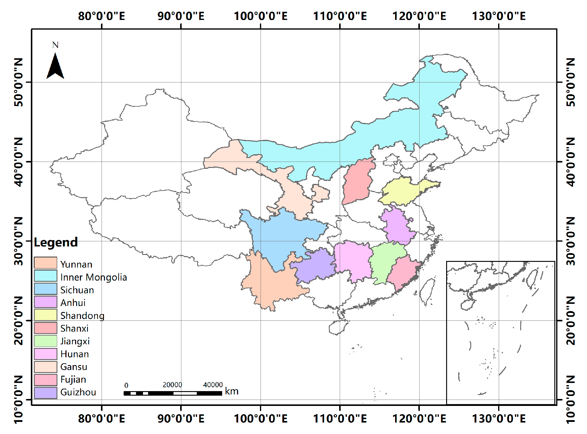
| Location (Province/Autonomous Region) | Species | Number | Ranges | |||
|---|---|---|---|---|---|---|
| DBH (cm) | Height (m) | Age (year) | ||||
| Sichuan | Pinus massoniana Lamb. | 44 | 0.35–59.27 | 0.3–40.09 | 5–112 | |
| Sichuan, Gansu | Abies fabri (Mast.) Craib | 16 | 0.25–45.9 | 0.11–27.3 | 5–161 | |
| Shandong | Platycladus orientalis (L.) Franco | 9 | 0.3–39.6 | 0.3–16.06 | 5–264 | |
| Jiangxi, Fujian, Hunan, Guizhou, Anhui | Cunninghamia lanceolate (Lamb.) Hook. | 388 | 0.35–42.95 | 0.3–30.5 | 5–106 | |
| Inner Mongolia | Larix gmelinii (Rupr.) Kuzen | 44 | 0.5–36.7 | 0.3–31.8 | 5–210 | |
| Shanxi | Larix principis-rupprechtii Mayr | 71 | 0.13–25.82 | 0.22–17.8 | 5–56 | |
| Pinus tabuliformis Carrière | 230 | 0.3–17.03 | 0.2–11 | 10–79 | ||
| Betula platyphylla Suk. | 75 | 0.03–23 | 0.2–13.2 | 5–80 | ||
| Populus davidiana Dode | 38 | 0.38–35.75 | 0.21–26.5 | 5–151 | ||
| Populus L. | 31 | 0.3–21.9 | 1–14.7 | 5–104 | ||
| Picea spp. | Picae asperata | 48 | 0.25–30.3 | 0.3–14.7 | 5–104 | |
| Picea meyeri Rehd. et Wils | 91 | 0.2–23.9 | 0.3–13.5 | 5–107 | ||
| Picea wilsonii Mast | 18 | 0.2–43.75 | 0.3–19.05 | 5–195 | ||
| Quercus spp. | Quercus aliena Bl | 11 | 0.3–23.8 | 0.4–18.5 | 5–79 | |
| Quercus dentata Thunb | 19 | 0.5–20.8 | 0.5–15.1 | 5–66 | ||
| Quercus wutaishansea Mary | 22 | 0.4–37.3 | 0.6–31.3 | 5–85 | ||
| Yunnan | Picea likiangensis (Franch) Pritz | 49 | 0.8–88.8 | 0.5–52.7 | 10–349 | |
| Pinus yunnanensis Franch. | 48 | 1.5–55.5 | 0.63–38.8 | 5–149 | ||
| Abies georgei Orr | 55 | 0.3–50 | 0.2–28.1 | 10–342 | ||
| Species | Location | R2 | SE | Height (b) | R2 | SE | DBH (b) |
|---|---|---|---|---|---|---|---|
| Abies fabri (Mast.) Craib | Sichuan | 0.986 | 0.065 | 1.174 | 0.986 | 0.069 | 1.273 |
| Gansu | 0.994 | 0.032 | 1.231 | 0.99 | 0.04 | 1.409 | |
| Cunninghamia lanceolata | Jiangxi | 0.945 | 0.009 | 0.8 | 0.906 | 0.012 | 0.78 |
| Fujian | 0.947 | 0.02 | 0.808 | 0.933 | 0.027 | 0.867 | |
| Hunan | 0.938 | 0.024 | 0.806 | 0.906 | 0.031 | 0.906 | |
| Guizhou | 0.98 | 0.026 | 0.931 | 0.969 | 0.003 | 0.973 | |
| Anhui | 0.914 | 0.066 | 0.927 | 0.922 | 0.069 | 0.926 |
| Species | R2 | SE | Height (b) | R2 | SE | DBH (b) |
|---|---|---|---|---|---|---|
| Quercus aliena Bl | 0.91 | 0.091 | 0.822 | 0.983 | 0.059 | 1.225 |
| Quercus dentata Thunb | 0.98 | 0.034 | 0.872 | 0.945 | 0.093 | 1.21 |
| Quercus wutaishansea Mary | 0.981 | 0.026 | 0.825 | 0.986 | 0.039 | 1.301 |
| Picea asperata Mast. | 0.977 | 0.032 | 1.568 | 0.885 | 0.077 | 1.949 |
| Picea meyeri Rehd. et Wils | 0.98 | 0.023 | 1.589 | 0.92 | 0.053 | 1.919 |
| Picea wilsonii Mast | 0.99 | 0.049 | 1.333 | 0.98 | 0.078 | 1.739 |
| Location | Species (Groups) | Height | DBH | ||||
|---|---|---|---|---|---|---|---|
| R2 | SE | b | R2 | SE | b | ||
| Sichuan | Pinus massoniana Lamb. | 0.969 | 0.025 | 0.823 | 0.984 | 0.025 | 1.008 |
| Sichuan, Gansu | Abies fabri (Mast.) Craib | 0.991 | 0.034 | 1.186 | 0.991 | 0.038 | 1.338 |
| Shandong | Platycladus orientalis (L.) Franco | 0.986 | 0.045 | 0.717 | 0.987 | 0.065 | 0.938 |
| Jiangxi, Fujian, Hunan, Guizhou, Anhui | Cunninghamia lanceolata | 0.952 | 0.009 | 0.82 | 0.93 | 0.001 | 0.829 |
| Inner Mongolia | Larix gmelinii (Ruprecht) Kuzeneva | 0.979 | 0.019 | 0.785 | 0.984 | 0.002 | 0.906 |
| Shanxi | Larix principis-rupprechtii Mayr | 0.949 | 0.032 | 1.348 | 0.918 | 0.045 | 1.578 |
| Picea spp. | 0.984 | 0.018 | 1.527 | 0.94 | 0.038 | 1.889 | |
| Quercus spp. | 0.965 | 0.026 | 0.842 | 0.966 | 0.041 | 1.250 | |
| Pinus tabuliformis Carrière | 0.975 | 0.012 | 1.065 | 0.968 | 0.02 | 1.306 | |
| Betula platyphylla Suk. | 0.959 | 0.022 | 1.016 | 0.962 | 0.028 | 1.356 | |
| Populus davidiana Dode | 0.94 | 0.03 | 0.981 | 0.964 | 0.033 | 1.405 | |
| Populus L. | 0.951 | 0.03 | 0.728 | 0.956 | 0.034 | 1.008 | |
| Yunnan | Picea likiangensis (Franch) Pritz | 0.994 | 0.015 | 0.885 | 0.995 | 0.015 | 0.842 |
| Pinus yunnanensis French. | 0.939 | 0.022 | 0.758 | 0.966 | 0.019 | 0.729 | |
| Abies georgei Orr | 0.997 | 0.016 | 1.016 | 0.996 | 0.02 | 1.089 | |
| Species (Groups) | BIAS | BIAS% | MAE | RMSE | RMSE% | R2emp | U2 |
|---|---|---|---|---|---|---|---|
| (m) | (m) | (m) | |||||
| Pinus massoniana Lamb. | 0.004 | 0.02 | 0.905 | 1.163 | 6.85 | 0.976 | 0.062 |
| Abies fabri (Mast.) Craib | 0.198 | 2.2 | 0.366 | 0.542 | 3.9 | 0.994 | 0.048 |
| Platycladus orientalis (L.) Franco | −0.036 | −0.411 | 0.317 | 0.410 | 4.88 | 0.993 | 0.043 |
| Cunninghamia lanceolata | −0.042 | −0.31 | 1.03 | 1.333 | 7.75 | 0.943 | 0.091 |
| Larix gmelinii (Ruprecht) Kuzeneva | 0.171 | 1.02 | 0.841 | 1.175 | 4.74 | 0.972 | 0.065 |
| Larix principis-rupprechtii Mayr | 0.096 | 1.3 | 0.657 | 0.83 | 11.24 | 0.961 | 0.097 |
| Picea spp. | 0.096 | 2.3 | 0.341 | 0.466 | 11.14 | 0.999 | 0.09 |
| Quercus spp. | −0.096 | −1.06 | 0.448 | 0.597 | 6.64 | 0.993 | 0.119 |
| Pinus tabuliformis Carrière | 0.128 | 2.193 | 0.452 | 0.670 | 11.45 | 0.952 | 0.101 |
| Betula platyphylla Suk. | −0.164 | −1.89 | 0.737 | 0.942 | 10.87 | 0.934 | 0.1 |
| Populus davidiana | 0.031 | 0.31 | 0.685 | 0.847 | 8.52 | 0.975 | 0.088 |
| Populus L. | 0.516 | 5.49 | 0.636 | 0.968 | 10.28 | 0.942 | 0.094 |
| Picea likiangensis | −0.177 | −0.72 | 0.669 | 0.848 | 3.48 | 0.995 | 0.031 |
| Pinus yunnanensis | −0.342 | −1.47 | 1.525 | 1.922 | 8.28 | 0.941 | 0.078 |
| Abies georgei Orr | −0.075 | −0.64 | 0.415 | 0.555 | 4.69 | 0.996 | 0.038 |
| Species (Groups) | BIAS (cm) | BIAS% | MAE (cm) | RMSE (cm) | RMSE% | R2emp | U2 |
|---|---|---|---|---|---|---|---|
| Pinus massoniana Lamb. | 0.326 | 1.53 | 0.972 | 1.368 | 6.44 | 0.987 | 0.056 |
| Abies fabri (Mast.) Craib | 1.85 | 10.17 | 1.852 | 2.257 | 12.41 | 0.946 | 0.109 |
| Platycladus orientalis (L.) Franco | 0.164 | 0.920 | 0.689 | 0.891 | 4.994 | 0.991 | 0.044 |
| Cunninghamia lanceolata | 0.231 | 1.35 | 1.605 | 2.158 | 13.66 | 0.912 | 0.116 |
| Larix gmelinii (Ruprecht) Kuzeneva | 0.209 | 1.23 | 0.874 | 1.123 | 6.59 | 0.984 | 0.058 |
| Larix principis-rupprechtii Mayr | 0.347 | 3.59 | 0.923 | 1.167 | 12.1 | 0.944 | 0.107 |
| Picea spp. | 0.431 | 5.19 | 1.012 | 1.333 | 16.05 | 0.884 | 0.145 |
| Quercus spp. | −0.059 | −0.47 | 0.664 | 1.066 | 8.42 | 0.983 | 0.064 |
| Pinus tabuliformis Carrière | 0.442 | 4.90 | 0.807 | 1.073 | 11.88 | 0.954 | 0.104 |
| Betula platyphylla Suk. | −0.262 | −2.75 | 0.836 | 0.998 | 10.5 | 0.953 | 0.094 |
| Populus davidiana | −0.159 | −1.16 | 0.883 | 1.057 | 7.68 | 0.982 | 0.066 |
| Populus L. | 0.606 | 6.85 | 0.761 | 1.02 | 11.53 | 0.955 | 0.1 |
| Picea likiangensis | −0.259 | −0.75 | 1.031 | 1.335 | 3.84 | 0.993 | 0.035 |
| Pinus yunnanensis | −0.603 | −2.1 | 1.333 | 1.567 | 5.45 | 0.983 | 0.05 |
| Abies georgei Orr | −0.086 | −0.36 | 0.827 | 1.158 | 4.82 | 0.995 | 0.039 |
| Species (Groups) | ||||||
|---|---|---|---|---|---|---|
| Quercus spp. | 12.94 | 146 | 0.3 | 0.23 | 21.92 | 10.59 |
| Betula spp. | 9.14 | 1112 | 0.2 | 0.15 | 12.03 | 5.94 |
| Larix spp. | 10.01 | 1070 | 0.24 | 0.16 | 15.01 | 7.89 |
| Pinus massoniana Lamb. | 5.91 | 1000 | 0.42 | 0.12 | 7.61 | 3.91 |
| Pinus yunnanensis | 4.77 | 410 | 0.25 | 0.08 | 5.85 | 3.09 |
| Picea asperata Mast | 9.87 | 385 | 0.24 | 0.16 | 7.5 | 3.87 |
| Abies fabri (Mast.) Craib | 11.65 | 308 | 0.24 | 0.18 | 9.53 | 4.81 |
| Cupressus funebris Endl. | 2 | 366 | 0.18 | 0.03 | 1.7 | 0.89 |
| Cunninghamia lanceolata | 7.26 | 1097 | 0.34 | 0.14 | 7.32 | 3.93 |
| Populus L. | 5.03 | 854 | 0.38 | 0.09 | 6.8 | 3.37 |
| Pinus tabuliformis Carrière | 0.66 | 161 | 0.31 | 0.01 | 0.94 | 0.5 |
| Other species | 68.53 | 8027 | 0.27 | 1.18 | 99.03 | 50.89 |
| Total | 147.77 | 14936 | -- | 2.53 | 195.24 | 99.68 |
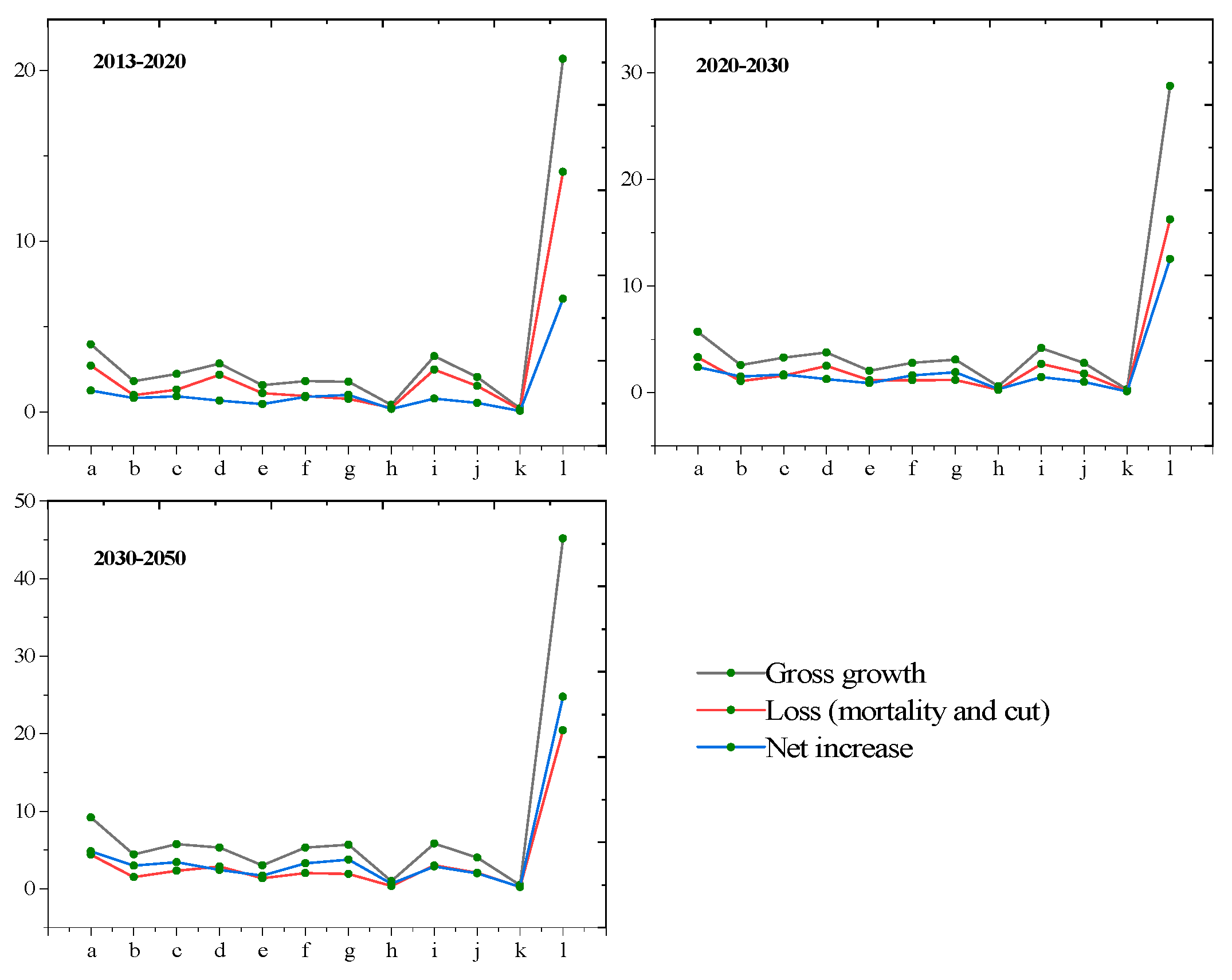
| Species (Groups) | |||||||||
|---|---|---|---|---|---|---|---|---|---|
| Growth | Loss | Increase | Growth | Loss | Increase | Growth | Loss | Increase | |
| Quercus spp. | 1.89 | 1.07 | 0.82 | 2.83 | 1.29 | 1.54 | 5.01 | 1.94 | 3.07 |
| Betula spp. | 2.22 | 1.31 | 0.91 | 3.29 | 1.58 | 1.71 | 5.76 | 2.34 | 3.42 |
| Larix spp. | 2.82 | 2.17 | 0.65 | 3.76 | 2.52 | 1.24 | 5.32 | 2.88 | 2.44 |
| Pinus massoniana Lamb. | 1.57 | 1.1 | 0.47 | 2.04 | 1.16 | 0.88 | 3.03 | 1.33 | 1.7 |
| Pinus yunnanensis | 1.8 | 0.94 | 0.86 | 2.79 | 1.16 | 1.63 | 5.31 | 2.02 | 3.29 |
| Picea asperata Mast | 1.77 | 0.78 | 0.99 | 3.1 | 1.2 | 1.9 | 5.68 | 1.92 | 3.76 |
| Abies fabri (Mast.) Craib | 0.41 | 0.23 | 0.18 | 0.59 | 0.26 | 0.33 | 1 | 0.35 | 0.65 |
| Cupressus funebris Endl. | 3.26 | 2.48 | 0.78 | 4.18 | 2.71 | 1.47 | 5.85 | 2.99 | 2.86 |
| Cunninghamia lanceolata | 2.04 | 1.52 | 0.52 | 2.76 | 1.76 | 1 | 4.03 | 2.06 | 1.97 |
| Populus L. | 0.22 | 0.15 | 0.07 | 0.32 | 0.19 | 0.13 | 0.52 | 0.27 | 0.25 |
| Pinus tabuliformis Carrière | 20.69 | 14.08 | 6.61 | 28.76 | 16.24 | 12.52 | 45.18 | 20.49 | 24.69 |
| Other species | 20.69 | 14.07 | 6.62 | 28.77 | 16.23 | 12.54 | 45.19 | 20.44 | 24.75 |
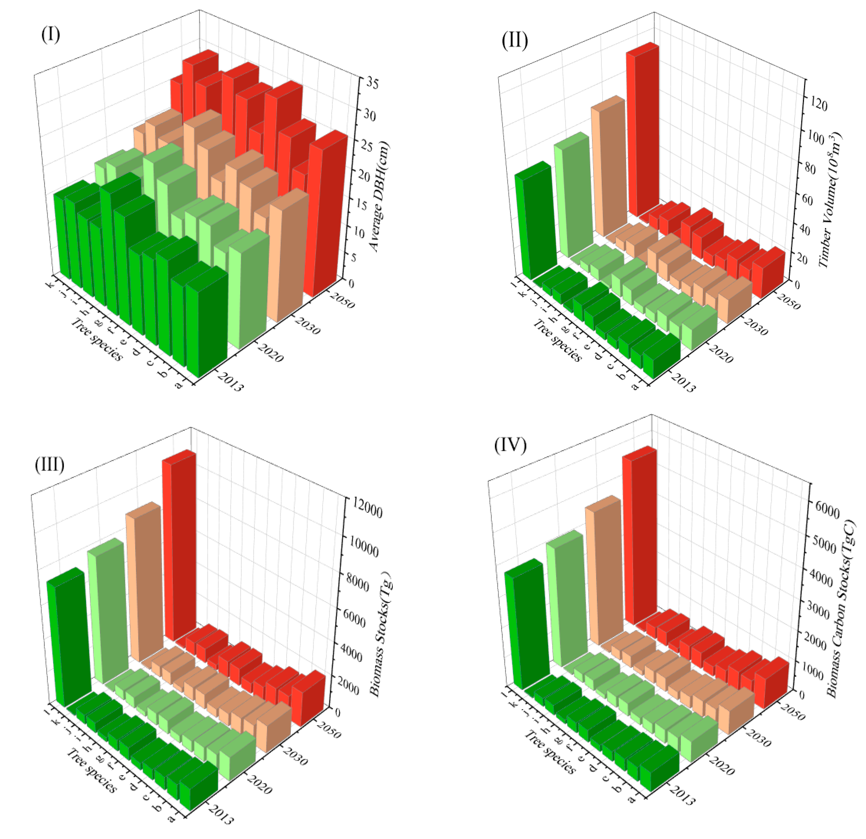
| Species (Groups) | D (cm) | B (Tg) | BCS (Tg C) | |||||
|---|---|---|---|---|---|---|---|---|
| 2013 | 2050 | 2013 | 2050 | 2013 | 2050 | 2013 | 2050 | |
| Quercus spp. | 14.94 | 26.02 | 12.94 | 21.39 | 1305.1 | 2116.09 | 630.63 | 1022.49 |
| Betula spp. | 14.08 | 21.38 | 9.14 | 14.57 | 950.53 | 1395.6 | 469.37 | 689.15 |
| Larix spp. | 16.75 | 25.48 | 10.01 | 16.05 | 785.67 | 1341.1 | 413.18 | 705.29 |
| Pinus massoniana Lamb. | 15.25 | 30.67 | 5.91 | 10.24 | 641.76 | 923.19 | 330.12 | 474.89 |
| Pinus yunnanensis | 14.35 | 23.6 | 4.77 | 7.82 | 416.54 | 632.87 | 219.98 | 334.22 |
| Picea asperata Mast | 19.26 | 28.2 | 9.87 | 15.65 | 786.16 | 1063.64 | 405.66 | 548.84 |
| Abies fabri (Mast.) Craib | 21.64 | 30.54 | 11.65 | 18.3 | 688.14 | 1040.68 | 347.51 | 525.54 |
| Cupressus funebris Endl. | 14.27 | 20.79 | 2 | 3.16 | 279.46 | 342.34 | 145.62 | 178.39 |
| Cunninghamia lanceolata | 14.29 | 26.94 | 7.26 | 12.37 | 636.59 | 907.31 | 341.53 | 486.77 |
| Populus L. | 15.67 | 29.61 | 5.03 | 8.52 | 575.08 | 826.59 | 285.01 | 409.66 |
| Pinus tabuliformis Carriifo | 14.76 | 26.25 | 0.66 | 1.11 | 73.84 | 108.59 | 39.24 | 57.7 |
| Other species | 14.73 | 24.66 | 68.53 | 112.36 | 7227.59 | 10891.71 | 3714.2 | 5597.16 |
© 2019 by the authors. Licensee MDPI, Basel, Switzerland. This article is an open access article distributed under the terms and conditions of the Creative Commons Attribution (CC BY) license (http://creativecommons.org/licenses/by/4.0/).
Share and Cite
Zhang, H.; Feng, Z.; Chen, P.; Chen, X. Development of a Tree Growth Difference Equation and Its Application in Forecasting the Biomass Carbon Stocks of Chinese Forests in 2050. Forests 2019, 10, 582. https://doi.org/10.3390/f10070582
Zhang H, Feng Z, Chen P, Chen X. Development of a Tree Growth Difference Equation and Its Application in Forecasting the Biomass Carbon Stocks of Chinese Forests in 2050. Forests. 2019; 10(7):582. https://doi.org/10.3390/f10070582
Chicago/Turabian StyleZhang, Hanyue, Zhongke Feng, Panpan Chen, and Xiaofeng Chen. 2019. "Development of a Tree Growth Difference Equation and Its Application in Forecasting the Biomass Carbon Stocks of Chinese Forests in 2050" Forests 10, no. 7: 582. https://doi.org/10.3390/f10070582
APA StyleZhang, H., Feng, Z., Chen, P., & Chen, X. (2019). Development of a Tree Growth Difference Equation and Its Application in Forecasting the Biomass Carbon Stocks of Chinese Forests in 2050. Forests, 10(7), 582. https://doi.org/10.3390/f10070582