Impact of Disturbances on the Carbon Cycle of Forest Ecosystems in Ukrainian Polissya

Abstract

Climate change continues to threaten forests and their ecosystem services while substantially altering natural disturbance regimes. Land cover changes and consequent management entail discrepancies in carbon sequestration provided by forest ecosystems and its accounting. Currently there is a lack of sufficient and harmonized data for Ukraine that can be used for the robust and spatially explicit assessment of forest provisioning and regulation of ecosystem services. In the frame of this research, we established an experimental polygon (area 45 km²) in Northern Ukraine aiming at estimating main forest carbon stocks and fluxes and determining the impact caused by natural disturbances and harvest for the study period of 2010–2015. Coupled field inventory and remote sensing data (RapidEye image for 2010 and SPOT 6 image for 2015) were used. Land cover classification and estimation of biomass and carbon pools were carried out using Random Forest and k-Nearest Neighbors (k-NN) method, respectively. Remote sensing data indicates a ca. 16% increase of carbon stock, while ground-based computations have shown only a ca. 1% increase. Net carbon fluxes for the study period are relatively even: 5.4 Gg C·year⁻¹ and 5.6 Gg C C·year⁻¹ for field and remote sensing data, respectively. Stand-replacing wildfires, as well as insect outbreaks and wind damage followed by salvage logging, and timber harvest have caused 21% of carbon emissions among all C sources within the experimental polygon during the study period. Hence, remote sensing data and non-parametric methods coupled with field data can serve as reliable tools for the precise estimation of forest carbon cycles on a regional spatial scale. However, featured land cover changes lead to unexpected biases in consistent assessment of forest biophysical parameters, while current management practices neglect natural forest dynamics and amplify negative impact of disturbances on ecosystem services.

1. Introduction

The functional ability of forest ecosystems to sequester carbon and provide other ecosystem services has been greatly altered by both direct and indirect impacts of climate change over the course of the last decades [1,2,3,4]. International efforts to mitigate global climate change demonstrate both evident progress and significant challenges to overcome due to the complexities of carbon cycle regulation worldwide, as well as substantial uncertainties in the mechanisms of its estimation [5]. The forests of Ukraine, covering nearly 16% of the country’s land area and providing a substantial carbon sink [6], have recently undergone changes and are very likely to face high climate, hydrology, and management-induced risks in the future [7]. Ukraine’s forests are situated in the mid-latitude ecotone, that is, in a transition area between the zone of temperate forests and forestless steppe: e.g., according to the abovementioned study [7], under certain climatic scenarios, a substantial worsening of growth conditions in Ukraine is forecasted by the end of this century mainly due to the water stress. This generates substantial spatial and landscape variability in their features and requires appropriate methods and approaches to account for the current and future vitality and carbon-sequestration capacity of forest ecosystems within the paradigm of adaptive sustainable forest management [8].

Natural disturbances are key drivers that substantially alter the spatio-temporal dynamics of forest ecosystems [9,10,11]: either stand-replacing wildfires, wind breakages and windthrow, or gap-scale insect outbreaks and disease affections. Many recent studies have reported on the exacerbation of disturbance regimes, which are explained by synergism between climate change and an increasing extent in the frequency and severity of natural disturbances [12,13]. An increasing variability of weather conditions results in more frequent and severe heat waves, which substantially escalate the mortality of trees and reduce the productivity of forests [14]. Interactions between different disturbance agents occur more frequently, mostly positively amplifying their negative impacts on ecosystems. Current management systems need to be adapted to already recognized changes in natural disturbance regimes [15].

The forest ecosystems of Ukraine are increasingly disturbed by a number of agents, which are mostly of biogenic origin (outbreaks of insects such as bark beetles and nematode worms; different diseases and pathogens, etc.), but also storms (windbreak and windthrow) and wildfires [16]. Sufficient systematic information on the impact of disturbances on carbon cycling in Ukraine’s forests is still lacking. Although somewhat complete aggregated countrywide estimates of the impacts of disturbances on the carbon budget of forest ecosystems are available, these are mainly related to the effects of harvest and wildfire [6,17]. However, regional analyses on the occurrence, extent and severity of disturbances are rare. For Ukrainian Polissya, the most forested zone in Ukraine’s flatlands, the only publications available to date concern the Chernobyl Exclusion Zone [18,19].

Salvage logging continues to have strong ecosystem consequences worldwide [20]. As the almost exclusive harvest method used in the forests of Ukraine’s flatlands, salvage logging is having an uncertain, but mostly negative impact on species diversity, processes of natural afforestation and the lives of local communities [21]. As this method of harvesting involves clear cutting aimed at reducing the risk of wildfires and insects spreading, they simultaneously neglect natural processes of forest dynamics and efforts to maintain biodiversity and other ecosystem functions [9]. To date, salvage and sanitary loggings drive main impact on managed forests after natural mortality events, while natural disturbances as prior reasons for such activities play a substantial role in the shaping of future spatial management composition.

While carbon sequestration seems to be the most important ecosystem service provided by forests in terms of climate change mitigation efforts, there is a lack of systematic application of carbon management in Ukraine. Full verified terrestrial carbon accounting is a fuzzy system that requires the complimentary use of different methods for the reliable assessment of uncertainties [5]. Major results obtained in Ukraine are based on a “semi-empirical” landscape-ecosystem approach, combining ground-based assessment with remote sensing data. Other approaches (eddy-covariance method, current generation of process-based models, and inverse modelling) have not been approbated in Ukraine. At the same time, process-based modelling at different scales (both forest landscape and dynamic global vegetation models) remains the only approach for the prediction of future changes in disturbance regimes and their impact on forest ecosystem productivity and services [22].

Studies on the biological productivity of forests are based on empirical methods that endeavor to obtain the most reliable data for past carbon sequestration potential [23]. While allowing the determination of the main carbon pools in ecosystems (live, dead biomass and soil) and some key carbon flows, this approach forms a solid basis for a full and verified accounting of the carbon budget of Ukraine’s forests.

The use of remote sensing (RS) data has been proven as a comprehensive tool for the mapping of forest cover, estimation of biomass, determining tree species distribution, and the assessment of past forest dynamics [24,25,26]. Using the common non-parametric methods Random Forest (RF) (as a processing application for the land cover classification of satellite imagery) and k-Nearest Neighbors (k-NN) (as a modelling system for the determination and calculation of forest parameters) provide strict, explicit, and reliable data on forest vegetation cover, live biomass and their parameters [27,28,29,30]. A number of studies based on remote sensing data assessed major natural disturbance agents across North America and reported large forest patches influenced by wildfires, windthrows and bark beetle outbreaks [31,32]. Meanwhile, European studies that focused on wind and bark beetle disturbances with smaller occurrence and severity, considered Landsat time series a reliable tool capable of assessing the disturbance agents mentioned above at 76%–86% precision in protected and actively managed stands [33,34]. Characterizing disturbances in forest ecosystems using satellite images has been proved to be successful tool for monitoring forest changes. Although dense time series of remote sensing data have been extensively used, a bi-temporal approach for the detection of disturbances is more preferential for use with commercial satellite images.

One of the background principles of transition to adaptive, risk resilient forest management in a changing world is a continuous monitoring of the state and dynamics of forest ecosystems with prompt application of new emerging knowledge of forest management practices. Such monitoring should be provided at different scales among which empirical studies at landscape level seem to be underestimated. A major objective of this research is to assess the carbon budget of forest ecosystems based on a relatively small experimental area over a 5-year period, using available ground and RS data. The study focused on ascertaining the role of natural and anthropogenic disturbances in the region with rapid changes of land cover and considers the influence of spatial and temporal peculiarities of data and methods on the reliability of the results. This requires carrying out a comparative analysis of different sources of available information and major agents that have influenced the local dynamics of forests over a short period.

Here we aim (i) to identify main typical disturbances in forest ecosystems of Ukrainian Polissya using ground-based inventory and remote sensing data; (ii) to assess impact of disturbances on carbon cycle and encompass links between natural and anthropogenic disturbances; (iii) to develop models and define impact of dead biomass decomposition on forest carbon cycle.

2. Materials and Methods

2.1. Study Area

The experimental polygon is located in the Chernihiv region between longitudes 31° 47′ 2″ E and 31° 52′ 60″ E and latitudes 52° 1′ 57″ N and 52° 5′ 31″ N (Northern Ukraine, Ukrainian Polissya zone), and covers an area of 45 km². Forest ecosystems, which covered 38.8% of the polygon area in 2010, comprised mostly Scots pine (Pinus sylvestris L.), silver birch (Betula pendula L.) and black alder (Alnus glutinosa L.)—respectively representing 44.7%, 39.8%, and 13.1% of the tree species dominance. Common aspen (Populus tremula L.) and other softwood broadleaved tree species dominate on a small area (~2.4%). Only 16% of local forest stands are mixed, 31% is a share of forests with admixtures of other tree species (less than 20% in stand tree composition), the rest is presented by stands with only one predominant tree species. Mixed stands are formed by combinations of all local common tree species. The experimental site represents a typical tree species composition for Ukrainian Polissya. A detailed description of the landscape, forest productivity and age distribution characteristics of vegetation was presented in Bilous et al. (2017) [30].

A distinct feature of the research area is the presence of continuous changes in land cover due to the natural afforestation of abandoned agricultural lands and illegal cutting by local people in shelterbelts within agricultural landscapes and forest stands on agricultural land. Forests per se are managed by a number of stakeholders (who are subordinate to the state forest authority) and are actively managed. Changes in forest cover may be very rapid: for example, areas affected by outbreaks of bark beetles, storms or wildfires, as a rule, are immediately cleared with salvage (sanitary) logging. The distribution of land cover classes within the study area during the years 2010–2015 is presented in

Table 1. Land cover distribution based on classification of satellite images.

Land Cover Class	2010		2015
	area, ha	%	area, ha	%
Forested area	1660	38.8	1866	43.7
Croplands	830	19.5	771	18.1
Grasslands	1473	34.5	1077	25.2
Shrublands	220	5.2	460	10.8
Wetlands	68	1.6	59	1.4
Water	16	0.4	34	0.8
Total	4267	100.0	4267	100.0

.

The occurrence of natural disturbance events across the experimental polygon was examined on a 5-year temporal scale (2010–2015). A large storm damaged forests on an area of 32.8 ha in the southern part of the study site in 2013, causing wind breakage in mostly pine and birch stands. Outbreaks of pests were observed throughout the polygon in 2010 and 2014, being caused by European spruce bark beetle (Ips typographus L.). In 2015, large fires occurred in the northeastern part of the polygon and some burned areas remained unmanaged during the above period, while the rest was cleared with salvage logging. Thus, the spatio-temporal structure of the research site represents a typical forest disturbance regime for Ukrainian Polissya [16].

2.2. Input Datasets

2.2.1. Remote Sensing Data and Ancillary Data

Remote sensing data for the study site included the following satellite images: RapidEye (acquisition date July 1, 2010; spectral bands used: B1—blue, B2—green, B3—red, B4—redEdge, B5—NIR4; spatial resolution—5 m); SPOT 6 (acquisition date August 9, 2015; spectral bands used: B1—blue, B2—green, B3—red, B4—NIR; spatial resolution—6 m); IKONOS (acquisition date August 12, 2011; resolution after pan-sharpening—0.81 m). All images have been acquired from data providers by end-user license agreements: BlackBridge, Airbus DS, and DigitalGlobe. We have chosen the images of 5–6 m spatial resolution since they enable effective mapping of forest disturbances within the study area and meet the requirements of national forest inventory guidelines regarding the size of minimal mapping unit of 0.5 ha.

Spectral bands of multispectral images have been converted to top-of-atmosphere (TOA) reflectance. RapidEye and SPOT 6 images were employed in the study for per-pixel classification, while IKONOS image was used as a source for training data collection. To improve the visual interpretation of IKONOS data, we applied the pan-sharpening technique for enhancing its spatial resolution up to 0.81 m. For geometrical correction of the images, we used rational polynomial coefficients (RPC) provided with data. Afterwards both RapidEye and SPOT 6 images were co-registered to IKONOS image which had higher spatial accuracy.

As a source of ancillary information, we employed digital elevation model (DEM) featuring a 10 m resolution and a vector layer which comprised polygons with soil types features within the study area. To match all components of the raster dataset, the DEM and RapidEye image were finally projected to a 6 m spatial resolution.

2.2.2. Reference Data

The sampling frame for image classification was created following a recommendation by Olofsson et al. [35] using a stratified sampling design. We used Global Forest Change dataset [36] for the stratification of the study area into four strata: permanent forest—forested area with canopy cover of 40% and more; non-forest areas; forest loss—defined as change from a forest to a non-forest state that occurred during the study period; and forest gain, which is defined as an opposite process to loss. The minimum sampling size for every stratum accounted for as much as 50 sampling points. All 568 sampling points were visually classified using IKONOS imagery as a reference. We applied a two-tier classification scheme representing the major land classes (LC) of the research area: croplands (263); forested area (246); shrublands (32); wetlands (9); and water bodies (19).

The second tier included a detailed classification of the forested area by dominant tree species. We used the forest inventory database (FID) to filter forest stands composed of a single species. Afterwards we selected about 150 random points within these stands (

Table 2. Training dataset for tree species classification.

Tree Species Code	Latin Name	Acronym	Sample Size
1	Alnus glutinosa L.	ALGL	22
2	Betula pendula Roth	BEPE	51
3	Pinus sylvestris L.	PISY	81
4	Populus tremula L.	POTR	6
5	Quercus robur L.	QURO	3
6	Robinia pseudoacacia L.	ROPS	3

). This step was important to exclude the mixed pixels problem from further analysis [37]. For each sampling point we extracted a median pixel within a radius of r = 12.62 m, which is a usual sample size for forest inventory in Ukraine.

The quality of the FID was crucial for our study because it was used as a reference dataset for prediction of carbon stock using satellite images. Three state forest enterprises whose forests are located within the boundaries of the research area were inventoried between three and seven years prior to our study. It was unclear if the inventory data corresponded to the current state of the forest cover. In addition, there was no information about forests outside areas managed by the state forest authority. In order to update and clarify the features of land cover, we conducted our own stand level inventory within the experimental polygon, regardless of its affiliation to local forest enterprises. The in-situ inventory was carried out according to the main requirements as set out in the existing Ukraine forest inventory manuals. During field inventory a qualified crew has inspected each forest stand and measured their main parameters: quadratic mean diameter, stand height, age, site index, relative stocking, and tree species composition. The mean stand parameters have been estimated by measuring diameters and heights of 3–5 sample trees within each forest polygon. For immature, mature, and overmature stands basal area has been calculated using circular (r = 12.62 m) and angle-counting plots (basal area factor 1). The selection of plot configuration depended on structure of a stand. For example, if a dense undergrowth was present in a stand making impossible to apply a relascope for tree counting, then fixed-radius plots were established. The number of sample plots (usually 3–7) has been estimated following the national forest inventory guidelines and depended on peculiarities of age, spatial structure and area of forest stand in question.

The purpose of the described inventory was twofold: (i) to clarify the boundaries of inventory units; and (ii) to precisely estimate forest stand biometrical parameters that are further used for satellite image classification. Thus, the training dataset for modelling the spatial distribution of carbon and net primary production (NPP) was created using FID and median pixel values for the forest stands selected above. We aggregated all pixels inside polygons to calculate the median values. The training datasets were collected separately for the years 2010 and 2015 using the RapidEye and SPOT 6 images.

2.2.3. Dataset for Biomass Estimation

The experimental data on forest dead biomass were collected at temporary sample plots (TSPs), which were established in accordance with the methodology proposed by Bilous (2014) [17]. TSPs are demarcated on site in accordance with the relevant national requirements for forest inventory sample plots. The size of a sample plot is defined based on the number of trees of the target species (usually not less than 200–250 trees for middle-aged and mature stands and 350–500 for young stands). The size of a TSP typically ranges from 0.05 to 1.00 ha. Diameter at breast height is measured for every tree. A total of 5–15 sample trees are selected proportionally to diameter class distribution. The sample trees are cut, based on their heights a height curve is further produced. Simultaneously, the following measurements are carried out: stem length from stump to top; height of stump; length of branch-free section of the stem; stem height at which the first live branch is attached, tree age, 5-year height increment of a tree, bark thickness and 5-year diameter increment at stump height, breast height (1.3 m), and at the middle of stem sections. For each sample tree dead branches are weighed. Snags were surveyed with measuring DBH, height, and identification of coarse and fine branches presence. Length and diameter on middle of length were measured in logs samplings, also presence of branches on downed stems was identified. Compartments of coarse woody debris (CWD) were determined by decomposition stage: snags (I-II classes), logs and coarse branches litter (I-V classes). Coarse branches litter and fine litter were assessed on sample plots. The biomass samples are further processed in a laboratory aiming at establishing density of the dead biomass components.

83 temporary sample plots were established in Ukrainian Polissya region with aim to model forest dead biomass, including 22 TSPs within the study polygon (5 in pine, 5 in birch, 5 in alder, and 7 in aspen stands). Additionally, we used data from 45 sample plots presented in Lakyda and Matushevych, 2006 [38].

These TSPs were used to assess the dry weight of dead biomass including snags, logs, coarse branches litter and fine litter (t d.m.·ha⁻¹), see

Table 3. Experimental data for forest dead biomass assessment (quantity of sample plots).

Experimental Data	Scots Pine	Silver Birch	Black Alder	Common Aspen
Temporary sample plots (TSPs), in total	19	77	16	16
Including estimation: snags	19	77	16	16
Logs	19	32	13	14
Coarse branches	19	33	13	14
Fine litter	19	33	13	14
Snag sample trees	72	84	48	48
Samplings, in total	792	840	525	704
Including: stems of snags	90	168	96	144
Logs	270	420	195	210
Coarse branches	270	84	195	210
Fine litter	162	84	39	140

. The applied classification and definitions of the dead biomass components are presented in

Table 4. Definitions of forest dead biomass components.

No.	Dead Biomass Component	Description	Size
1	Snags	Standing stems over bark and branches of dead and live trees, if their height is >1.3 m	No limitations
2	Logs	Downed stems over bark or their parts with branches, including stumps with a height <1.3 m	No limitations
3	Litter of coarse branches	Downed branches over bark, broken from stems of live or dead trees	Diameter >1 cm
4	Fine litter	Foliage (leaves and needles), fine branches, bark, fruits and seeds on the ground	Diameter of branches ≤1 cm

.

The dead biomass of tree and shrub roots was not assessed due to the large uncertainty associated with the identification of different decomposition stages (dead roots versus decomposed soil organic matter). The total aboveground dead biomass of the experimental polygon’s forests was computed as the sum of snags, logs, coarse branches and fine litter.

2.2.4. Data on Heterotrophic Soil Respiration

Soil carbon stock (for the stock-based method) and heterotrophic soil respiration (HSR) (for the flux-based method) were obtained based on the database of Mukhortova et al. [39]. Of the nine main soil groups typical for the forest ecosystems of Eurasia, only three were found among the soil types of the experimental polygon (

Table 5. Heterotrophic soil respiration (HSR) input data for the study region.

Group of Soils	HSR, g C·m−2·year−1
Luvisols and Greyzems—texture-differentiated soils	290 ± 160
Gleysols—over wetted mineral soils with thick (10–30 cm) organic horizon	314 ± 214
Histosols—over wetted organic soils	268 ± 201

).

2.3. Analyses

We have performed data analysis in the two directions. Forest inventory data has been used for estimation of mean and total C and NPP values. With aim to obtain these values, data was aggregated on stand scale; inventory database and geostatistics methods were used. As an alternative, estimated C and NPP values were compared to data obtained from satellite images. The forest mask was created through classification of images using the RF method, while NPP and C values were predicted within the mask by means of the k-NN method. Since these maps are of raster type, assessment of the mean values for fluxes and stocks has been carried out based on the pixel values. These data have been aggregated by the tree species mapped within the study area. The analyses are presented separately for the years 2010 and 2015 to enable estimation of C fluxes. We have also calculated the uncertainties for the predicted results within the two outlined directions of the data analysis.

2.4. Data Processing Methods

2.4.1. Image Classification Approaches

We used a Random Forest classifier to classify images. We used the following variables as predictors in the LC classifications: X and Y coordinates, DEM, and spectral bands. The out-of-bag error for the forest mask was about 2%. There are two sources of commission and omission errors, namely shrublands and orchards, that have spectral features similar to those of forests. The confusion in terms of tree species classification is larger, so we included the ground forest type as an additional predictor variable. This helped us to distinguish black alder more precisely. The total accuracy of tree species classification was 13%.

We used %IncMSE as a measure of variable importance for tree species classification. Among spectral data, red, red edge and near-infrared bands were the most important variables (Figure 1 and Figure S1), while those from a non-spectral features list represents DEM and soil type. As was expected, coordinates X and Y did not play a significant role in tree species classification.

As can be seen in Figure 1, coniferous and deciduous forests are distinguished quite well. The major confusion occurs between black alder and silver birch that have similar spectral signals in visible and infra-red bands. We included the soil type layer to improve our classification (Figure 2 and Figure S2). The forested area lies within eight soil types that could be grouped in two major classes: Luvisols and Greyzems (soil types 2, 3, 6, 8, 10, 133, 162; [39]) and Hystosols (soil type 138). Figure 2 demonstrates that black alder mainly occupies over wetted organic soils (Hystosols), while silver birch never occurs there.

To predict the spatial distribution of carbon stock and NPP at pixel basis we used the k-NN technique available from the yaImpute package for R [40]. Spectral bands and DEM were selected as predictors. We analyzed all available distance metrics (Euclidean, Mahalanobis, Most Similar Neighbor, Gradient Nearest Neighbor, Individual Component Analysis) and selected Random Forest as a method for the nearest neighbor search since it was more precise. We imputed carbon and NPP values for each pixel of RapidEye and SPOT 6 images using the corresponding training datasets for 2010 and 2015. The imputation was performed strictly within the forest masks.

The spatial accuracy of forest masks for 2010 and 2015 was estimated using an error matrix of land cover classification (

Table 6. Confusion matrix of land cover classification for 2010.

Reference Data	Classified Data						Class Error 1
	Croplands	Forests	Grasslands	Shrublands	Water Bodies	Wetlands
Croplands	113	1	16	1	0	0	0.137
Forests	0	242	2	0	0	0	0.016
Grasslands	28	3	96	4	0	0	0.267
Shrublands	4	0	26	2	0	0	0.937
Water bodies	0	1	0	0	18	0	0.053
Wetlands	0	2	1	0	0	6	0.333

¹ Out-of-bag (OOB) estimate of error rate: 16.0%.

and

Table 7. Confusion matrix of land cover classification for 2015.

Reference Data	Classified Data						Class Error 2
	Croplands	Forests	Grasslands	Shrublands	Water Bodies	Wetlands
Croplands	114	1	15	2	0	0	0.130
Forests	1	240	1	4	0	0	0.024
Grasslands	21	0	101	8	0	1	0.230
Shrublands	0	4	14	14	0	0	0.562
Water boodies	0	0	0	0	19	0	0.000
Wetlands	0	0	0	0	0	9	0.000

² OOB estimate of error rate: 12.5%.

). We used out-of-bag (OOB) samples as implemented in the RF classifier to assess the misclassification between reference and predicted land cover classes.

The OOB error rate of 12.5% proved that SPOT-based classification of land cover outperformed RapidEye classification by more than 16% of the OOB error. The user accuracy of forest cover classification for both epochs reached 97%–98%.

The total accuracy of the tree species classification is significantly lower and estimated as high as 78% for both 2010 and 2015. The major source of misclassification is caused by three tree species that cover a relatively small area within the study polygon (aspen, oak, and black locust).

2.4.2. Carbon Budget Estimation

Aiming to estimate carbon flows, we applied the methodology of full verified carbon accounting developed by the International Institute for Applied Systems Analysis (IIASA, [5]). Using both stock-based and flux-based methods, we examined the available data from the ground-based surveys on the sample plots and FID, as well as the dataset presented by Mukhortova et al. [39] for soil carbon stock and heterotrophic respiration estimation. Classic methods of statistics and error theory were used for calculation of the main parameters of output results of carbon budgets and fluxes. The uncertainty of indirect measurements was estimated at a probability of 68% (±SD).

The stock-based method is defined as:

$$\Delta C=\Delta LB+\Delta WD+\Delta S$$

(1)

where ΔC is the annual change of organic carbon in forest ecosystems, while ΔLB, ΔWD, and ΔS respectively represents changes of C stocks in live biomass, woody detritus and soil.

The method of dead biomass estimation in Ukraine proposed by Bilous [1] is a modification of Harmon et al. [41]. This approach defines coarse woody debris (CWD) as snags (standing dead stems and dead branches on live and dead trees), logs (fallen stems and stumps) and coarse branches (d > 1 cm) litter, while other dead biomass components (fine litter of fine branches (d ≤ 1 cm), fruits and foliage, and dead roots) are considered part of soil carbon stock.

The flux-based method can be defined as:

$$NBP=NPP-HSR-DIST-LAT-DEC$$

(2)

where NBP and NPP represents net biome and net primary production respectively, HSR is heterotrophic soil respiration, DIST is the loss caused by natural and anthropogenic disturbances, LAT is lateral fluxes into the lithosphere and hydrosphere, and DEC is carbon loss caused by the decomposition of woody detritus.

Carbon fluxes related to harvest and natural disturbances are jointly accounted for due to the above-mentioned clearing of post-disturbance areas by salvage logging (except for young stands after wildfires). LAT flux due to the actual absence of respective data was calculated using the same assumption proposed by Shvidenko et al. [16] for Ukraine, being given as 5% of NPP flux for study area.

For live biomass estimation (birch, alder, and aspen) we used equations proposed by Bilous et al. [30], which include stems over bark, branches, foliage, understory and green forest floor. Belowground live biomass was defined using models presented in Shvidenko et al. [42]. All the equations used include stand age, site index and relative stocking as independent variables.

Dead biomass by components were calculated using Equations (3)–(5):

$$D{B}_{fr}=a_0·D^{a_1}·H^{a_2}·RS{t}^{a_3}$$

(3)

$$R_{fr}=\raisebox{1ex}{$D{B}_{fr}$}\!\left/ \!\raisebox{-1ex}{$GS$}\right.=a_0·D^{a_1}·H^{a_2}·RS{t}^{a_3}$$

(4)

$$D{B}_{fr}=a_0·D^{a_1}·H^{a_2}·RS{t}^{a_3}·\exp (a_4·D+a_5·RS)$$

(5)

where DB_fr is mean dead biomass (t·ha⁻¹), R_fr is the dead biomass expansion factor, GS is growing stock volume (m³·ha⁻¹), D is mean diameter (cm), H is mean height (m), and RSt is relative stocking.

Dead biomass of pine, birch, aspen and alder was defined by Equation (3), fine litter in birch stands by Equation (4) and coarse branches litter in pine stands by Equation (5). The statistical characteristics of forest dead biomass equations are presented in Appendix A.

The decomposition model for CWD is defined as:

$$DEC=S·k_1+\left(L+CL\right)·k_2$$

(6)

where S is C stock in snags, L represents logs, CL is C stock in litter of coarse branches and k₁ and k₂ are the respective decomposition annual rates computed as a single exponential function.

In order to estimate the decomposition rate, we collected 317 samples of CWD of birch, alder, aspen, and oak. Of these, 153 were between 1 and 10 cm in diameter, and 164 had a diameter of more than 10 cm at different stages of decay. For each CWD sample, diameter and density were measured in dry conditions, given that the dates of the respective tree deaths were known.

The decomposition rate of CWD was assessed using the chronosequence method [43]:

$$P_t=P_0·e^{-k·t}$$

(7)

where P_t is the density of CWD remaining at time t (years), P₀ is the initial density, and k is the average annual constant of the decomposition rate independent on the climatic conditions (year⁻¹).

Decomposition rates for birch, alder, aspen and oak are presented in Appendix A. The decomposition rate of snags for all other tree species was taken at 0.03 year⁻¹, and for logs of Scots pine at 0.06 year⁻¹ according to Shvidenko et al. [16].

NPP was accounted for using a semi-empirical method described in Shvidenko et al. [42]. In this method, NPP is considered to be the difference of total productivity of live biomass for two consecutive years, taking into account the turnover of fine roots and foliage, as well as damage by wind, insects, harvest, etc. Contrary to the direct aggregation of field measurements, this method does not have any recognized biases. The uncertainty of NPP was defined independently through a correlation between the current increment of live biomass and NPP.

As a rule, insect outbreaks and wind damage cause relatively small impacts on biomass stock, converting a part of live biomass into dead organic matter and decreasing the biological productivity of the remaining over- and understory [9]. Such natural disturbances were observed in the study area for the considered time period, however, the disturbed sites are usually cleared with removal of all biomass except for underground live and dead components. Fires that occurred on the polygon area were observed in three stands, including a complete aboveground biomass loss due to high-severity burning in young pine forests (two stands, with a few snag remnants) and was cleared by salvage logging the site of the third stand. Hence, all the natural disturbances in this study were considered a net total loss of entire accumulated aboveground biomass, which was similar to our calculations for harvested forest stands.

3. Results

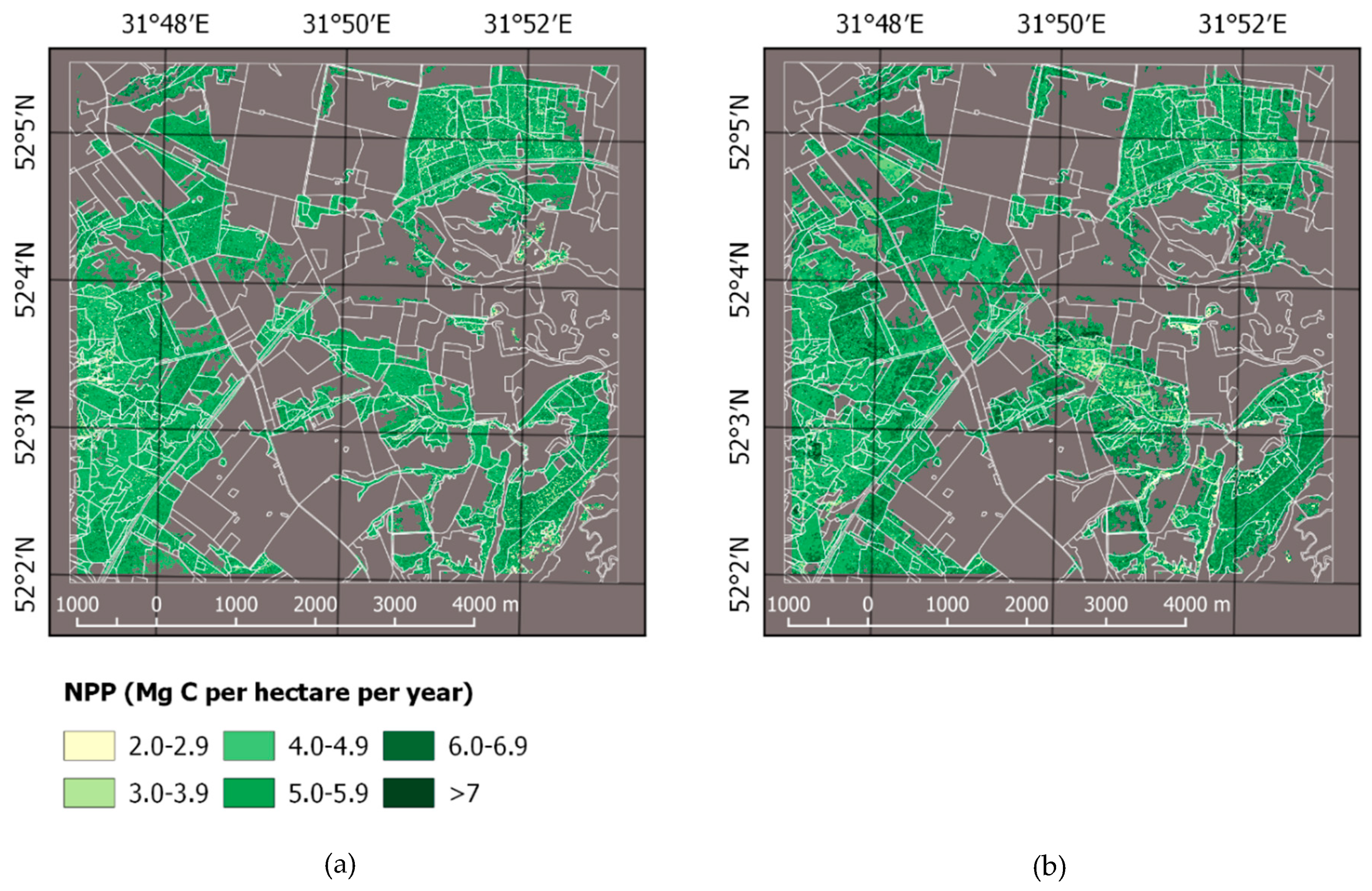
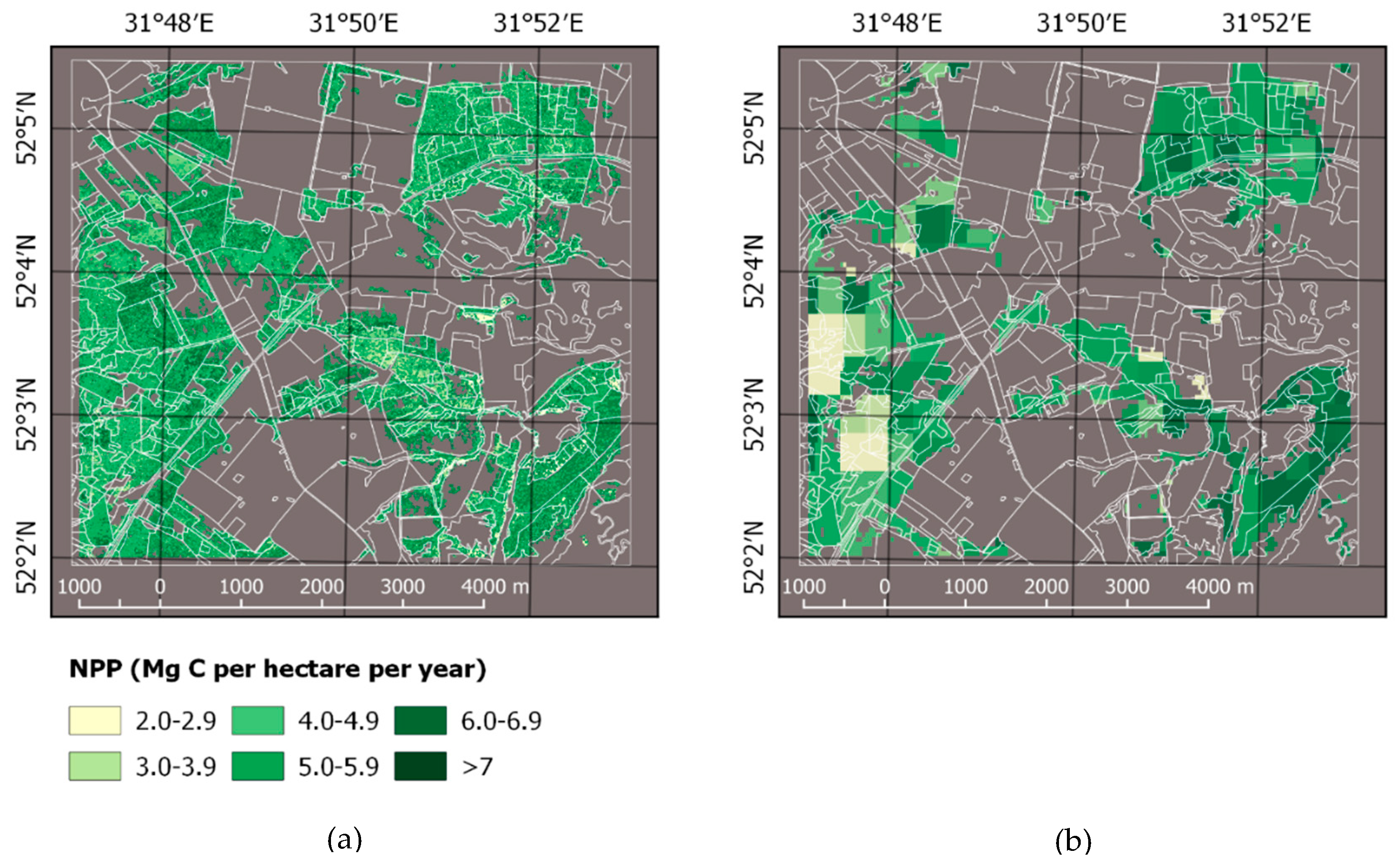
3.1. Forest Mask, Carbon Stock, and NPP

FID showed a slight decrease in the area covered by pine (commonly harvested for timber production) and a corresponding increase in birch-dominated stands (as a pioneer species encroaching abandoned agricultural sites), while the area dominated by alder, which prefers wetter soils with a thin (<30 cm) peat layer, has not actually changed. C stock has slightly increased for all main species indicated by FID but has shown great fluctuations in RS estimates as well as in pine-dominated forests (

Table 8. Tree species distribution: Forested area and carbon stock, 2010–2015. FID: forest inventory database; RS: remote sensing.

Species	Area, ha				Carbon, Gg C
	2010		2015		2010		2015
	FID	RS	FID	RS	FID	RS	FID	RS
Black alder	240 ± 5	202 ± 43	245 ± 5	231 ± 49	11.1 ± 0.7	7.9 ± 2.6	12.5 ± 0.8	13.4 ± 4.6
Silver birch	711 ± 14	614 ± 86	725 ± 14	681 ± 95	29.4 ± 1.6	25.7 ± 5.5	31.2 ± 1.7	36.4 ± 7.9
Scots pine	866 ± 17	829 ± 92	831 ± 17	928 ± 103	66.2 ± 3.3	66.0 ± 11.0	69.7 ± 3.4	82.2 ± 14.0
Common oak	13 ± 1	5 ± 3	13 ± 1	2 ± 2	1.2 ± 0.11	0.3 ± 0.2	1.3 ± 0.12	0.1 ± 0.1
Common aspen	13 ± 1	1 ± 1	14 ± 1	23 ± 9	1.0 ± 0.12	>0.1	1.1 ± 0.13	1.3 ± 1.3
Black locust	6 ± 1	9 ± 6	6 ± 1	1 ± 1	0.4 ± 0.05	0.7 ± 0.7	0.4 ± 0.05	>0.1
Total	1849 ± 23	1660 ± 129	1834 ± 23	1866 ± 146	109.3 ± 5.9	100.7 ± 11.6	116.2 ± 6.3	133.5 ± 15.7

, Figure 3).

Forest gain (Appendix A, Figure S5) is observed on abandoned agricultural lands as well as on clear-cuts, since regeneration was established before 2010. Young stands on abandoned agricultural lands are characterized by intensive tree growth and increasing biodiversity [44].

Forest loss (

Table 9. Forest gain and loss, 2015.

Direction of Change	Area, ha		Carbon, Gg C
	FID	RS	FID	RS
Gain	68	304	0.7	17.0
Loss	103	108	8.2	7.1
Net change	−35	+196	−7.5	+9.9

) is identified within forested areas disturbed by natural agents (a wildfire in the north-east, a wind breakage in the south-west and insect outbreaks throughout the polygon) that have been consecutively cleared by salvage logging, as well as by stands harvested for timber production or as a result of illegal logging in forests of different subordination.

A comparison of outputs demonstrates the opposite results: the increase of net forested area according to RS data is 5.6 times larger than the respective loss obtained from FID. Carbon stock calculation results show a considerable variation from net loss to net gain according to field inventory and remote sensing data.

The same trends are recognized for NPP estimates (

Table 10. Net primary production by species, 2010–2015.

Species	NPP, Gg C·year−1				Average NPP, Mg C·ha−1·year−1
	2010		2015		2010		2015
	FID	RS	FID	RS	FID	RS	FID	RS
ALGL	1.2	0.8	1.2	1.0	4.9	4.6	4.8	5.0
BEPE	3.5	3.0	3.5	3.2	5.0	4.9	4.7	4.8
PISY	4	3.7	3.9	4.4	4.6	4.5	4.8	4.8
QURO	>0.1	>0.1	0.1	0.1	4.9	5.0	5.5	5.4
POTR	0.1	>0.1	0.1	>0.1	4.1	3.9	4.7	4.7
ROPS	>0.1	>0.1	>0.1	>0.1	3.9	4.2	4.3	4.8
Total	8.8	7.6	8.8	8.7	–

, Figure 4 and Figure S6).

3.2. Carbon Budget Estimation and Disturbances Impact

Soils, including fine litter, store the largest amount of C. Estimates of C stock strictly depend on the size of the forested area, which was much larger for RS data, leading to a substantial increase of total C stock in soils and live biomass (

Table 11. Stock-based C changes, 2010–2015.

Ecosystem Components	Carbon stock, Gg C
	FID			RS
	2010	2015	Changes, %	2010	2015	Changes, %
Live biomass	96.3 ± 3.5	103.0 ± 3.8	+7.0	87.6 ± 15.1	116.2 ± 20.2	+32.6
Woody detritus	6.0 ± 1.0	6.2 ± 1.0	+3.3	5.4 ± 1.6	7.2 ± 2.2	+33.3
Soil	461.0 ± 253.6	458.2 ± 252.0	−0.6	416.2 ± 228.9	468.4 ± 257.6	+12.5
Total	563.3 ± 253.6	567.4 ± 252.0	+0.7	509.2 ± 229.4	591.8 ± 258.4	+16.2

). On the other hand, since a change of forested area on abandoned agricultural sites was not accounted for by FID, the calculated soil C stock has slightly decreased, resulting in a high discrepancy (~20 times) between the two stock-based outputs obtained by different methods.

Dead biomass (including CWD and fine litter) on average account for 13.0% of the total C in forest biomass within the study area, with a 41.5% C share of woody debris (Appendix A, Figure S7). The percentage of belowground live biomass is slightly higher (16.9%) while green forest floor and understory both represent around 3.0% of the total biomass stock. Apparently, local C stock is concentrated in stem over bark (58.2%) compartment, while foliage and live branches account for 8.9% of C stock.

HSR fluxes were strictly related to the size of the forested area, while the resulting DEC were dependent on stored woody debris. The discrepancy between FID and RS data computed using the flux-based method was insignificant, specifically in comparison to the respective values obtained using the stock-based method (

Table 12. Flux-based C changes, 2010–2015.

Carbon Fluxes of Forest Ecosystems	Annual Value of Flux (Except DIST), Mg C year−1
	FID		RS
	2010	2015	2010	2015
Net primary production (NPP)	8886 ± 678	8750 ± 671	7748 ± 1262	9008 ± 1498
Heterotrophic soil respiration (HSR)	5340 ± 3364	5320 ± 3352	4778 ± 3345	5371 ± 3760
Decomposition of CWD (DEC)	297 ± 91	303 ± 91	336 ± 147	360 ± 160
Lateral fluxes into lithosphere and hydrosphere (LAT)	444 ± 333	438 ± 329	387 ± 290	450 ± 338
Loss caused by natural disturbances and harvest (DIST)	8311 ± 1247		7073 ± 2334
Net	+5426		+5610

).

All fluxes except DIST are presented as annual values for 2010 or 2015, while losses caused by disturbances and harvest were computed for the entire study period.

Overall, the results of the NPP assessment obtained from FID and RS data are consistent. However, the RS data addresses a stronger trend of increasing NPP. This may be explained by a more flexible NPP estimation for each RS imagery pixel compared to a rougher stand-wise assessment.

RS data showed less C loss caused by disturbances, since this method estimates the forest cover area more flexibly, while FID is typically based on a polygonal approach.

The temporal composition across disturbance agents and gain by area/carbon change, being based on annual forest inventory data on replanting and salvage/sanitary loggings that have occurred within study period, is presented in Figure 5 and Figure S8.

Values for 2010 and for 2015 are presented for July 31, 2010 and 2015, respectively.

The increase in forested area follows from the transformation of previously unforested area to forests (after a reforestation phase reaches the 5-year mark), explains the substantially lower respective C values. A similar situation is observed on burned areas as a result of the disturbance followed by salvage logging, particularly in young stands. Harvest, however, remains the primary cause of C and forested area loss. At the same time, an intensive storm event in 2013 actually converted the entire experimental polygon from a net C sink to a net C source causing ~2 Gg C emissions (Figure 5 and Figure S8).

4. Discussion

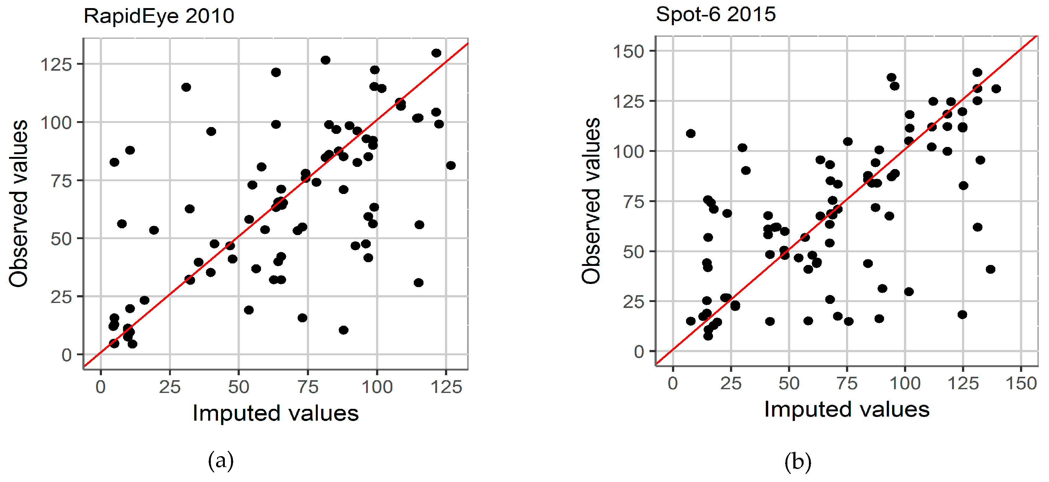
4.1. Spatial Accuracy and Reliability

The observed and estimated values of total carbon stock show substantial variability but on average, they are well agreed with the 1:1 line (Figure 6 and Figure S9).

The per-pixel distribution of NPP values for 2015 were compared using the regional map compiled by Lesiv et al. [6] with a spatial resolution of 40 × 60 m (Figure 7 and Figure S10). Although the compared maps have different spatial accuracy, we can conclude that the regional map performed well for such a small area. We compared the mean values of NPP estimates—4.9 Mg C·ha⁻¹·year⁻¹ according to the map presented in Lesiv et al. [6], while our estimate is 4.8 Mg C·ha⁻¹·year⁻¹.

We applied the lossyear layer of the GFC dataset [36] to calculate forest loss that occurred within the study area during 2011–2015 (Figure 8 and Figure S11). The global forest change map underestimates the area of forest loss. Although, the loss layers of this research and GFC have a rather good agreement—the total GFC loss is nearly 60 ha while, according to our assessment, it is 137 ha, which is explained by the rough spatial resolution of GFC data.

GFC data does not provide information about an annual forest gain but it includes a cumulative area that has been converted from non-forested into forested during the period from 2000 to 2015. For the study period, about 314 ha of forest gain is identified by GFC. We classified about 318 ha of forest gain for the same period.

4.2. Forest Land Cover and Carbon Estimation

Ukraine still does not have an effective enough forest inventory and management system capable of meeting global change challenges. In total, 7.5% of Ukrainian forests are not officially subordinated to any entity [45]. The last aggregated forest inventory data for Ukraine was reported in 2011, while a countrywide national forest inventory has not been carried out yet [45]. In addition, rapid changes in land cover induce additional uncertainties. This situation is clearly illustrated by the research polygon. According to FID the percentage of forest cover there was 40.7% in 2015. However, according to our surveys, forests of state enterprises in the region only account for 26.5%, while the remaining forest cover consisted of young forests under natural succession processes on former agricultural lands, which had not been used for the preceding 20–30 years. During 2010–2015 there was an active regrowth of trees and shrubs on abandoned agricultural lands [29].

However, a simultaneous deforestation process took place there. Aiming to reclaim land for agricultural use, trees and stands were cut on an area of about 200–250 ha. Note that this land was not indicated as forest in 2010. The natural regrowth on those sites was at canopy closure stage (turning into forest as land cover class) in 2011–2012, the majority of it was harvested (occasionally being burned) in 2013–2014 and the territories were prepared for crop planting. Such forests were not indicated in either FID or RS data in 2010 and 2015.

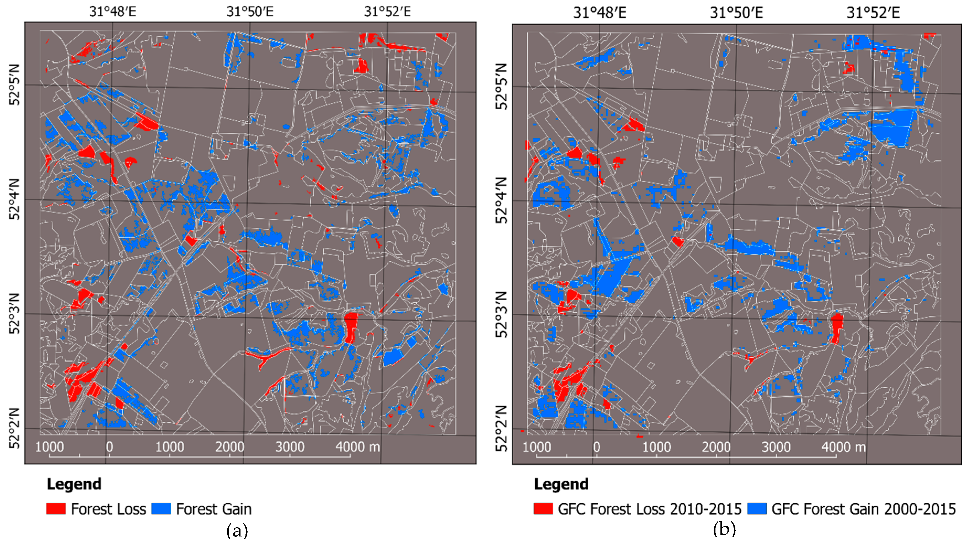
4.3. Disturbances Impact

The extent, frequency, and severity of individual natural disturbances like wildfires, wind damage, and bark beetle outbreaks in the study region have a very uneven temporal distribution. This unevenness is substantially amplified by post-disturbance forest management activities. For instance, practically all stands affected by bark beetles are cleared by salvage logging. As a result, these stands become agents of biomass and C loss. Only a few forested areas damaged by insects and diseases were found in the study area during the 5-year period. Note that the spatial structure of forest cover may play a substantial role in the distribution of disturbances and carbon fluxes. For instance, young stands of silver birch serve as a buffer zone that restricts the spreading of bark beetles that actively damage Scots pine stands [46].

An intense storm event in 2013 destroyed forests over 32.8 ha (~1.8% of forested area) of the research polygon and made them a net C source for this year (considering C budget of forested areas within polygons and its C fluxes), in spite of the forest gain and increasing productivity of existing stands. Information about wood lateral flow in the region is lacking or unreliable. Therefore, the substitutional effect of sanitary (salvage) logging on the C cycle cannot be estimated precisely in the study region. On the other hand, timber obtained from such harvesting in Ukraine is basically used as fuel. Consequently, biomass removal caused by wind breakages and insect outbreaks (where all plots were cleared) was estimated as a net C loss. Comparing to studies with similar geographic, climatic, and hydrological conditions and tree species compositions, we can call for resent study from Polish forests [47]. There was a data on severe wind breakages that had removed .ca half of stand basal area in forests of Scots pine, Silver birch and Black alder. However, post-disturbance ecosystems not affected by salvage loggings created more structurally diverse stands with better maintaining the habitats preservation function.

Different post-disturbance forest management actions may also play a substantial role. Forests within the study area are subordinated to three state or communal authorities, however, clear cuts were carried out after outbreaks of pests or diseases only in one enterprise. In two others, selective sanitary cuts that caused smaller carbon emissions were carried out. Such case may refer to situation occurred in post-soviet countries of Eastern Europe without long history of non-state forestry: e.g., in Poland private forests faced much more frequent natural disturbances, which can correspond to lower ecosystem resilience entailed by inappropriate management practices [48].

Therefore, local disturbances are mainly linked to human factor, while natural events serve as preliminary reasons for either salvage or sanitary loggings in stands of all age cohorts starting from middle-aged forests. However, Ukrainian forests planted in second part of XX century remain to be ecosystems with low resilience capacity [7], so thus needing human intervention after prior mortality events with aim to prevent risks related to further occurrence and spreading of bark beetles and diseases. So we are therefore convinced that for such cases the composition of natural disturbances that caused obliged human silvicultural activities like salvage logging must be determined. Another question is how loggings after natural disturbances with such intensity and actual absence of natural concerns affect local biodiversity and ecosystem functioning [49].

In general, consideration of regional specifics increases the reliability of estimates of carbon cycling in forest ecosystems. However, some limitations remain. Some changes in land and forest cover occur so rapidly that they cannot be properly quantified, even over short time periods. In addition, unrecognized biases could be generated due to the fact that regional models and empirical aggregations applied within this research, are inevitably based on limited experimental data collected on a restricted number of sample plots.

Summing up, we state that natural and anthropogenic disturbances caused nearly 21% of total C emissions from forest ecosystems in the study area from 2010 to 2015, including 57% due to timber harvest and 34% due to wind damage, while 6% resulted from insect outbreaks and 3% from wildfires. The persistence of this kind of distribution is very unlikely due to the substantial impacts of rare disturbances of large magnitude (e.g., wind damage or a fire that occurred during the study period).

5. Conclusions

Some lessons follow from this study. Official forest inventory data in Ukraine are not capable of properly reflecting the short period dynamics of forests. There are two major reasons for this, namely, the incompleteness of territorial coverage and the impossibility of accounting for rapid (1 to 3 years) changes in land cover. This generates a bias of unknown direction and magnitude. Carbon emissions caused by insects and diseases are substantially dependent on forest management similarity and appropriateness (e.g., selective harvest versus clear cutting). Inappropriate forest management (e.g., unreasonable clear cuts in stands affected by biogenic agents) usually increases carbon emissions. The impacts of disturbances like harvest and insect outbreaks are the major drivers of forest cover dynamics in Ukrainian Polissya. Rapid changes in land and forest cover are an inherent feature of this most forested region of the country’s flatlands. This also greatly influences the functions and services of forest ecosystems, particularly their carbon cycle. Wildfires and storms may also have a substantial impact on carbon emissions. However, the extent, frequency, and severity of these disturbance agents are not systematic on a local spatial and short temporal scale. Overall, this study raises some questions about the scaling aspects of a full verified carbon account of forest ecosystems. The most pressing of these are, how regional changes occurring at temporal and spatial scales that are impossible to properly monitor by large territorial assessments impact the reliability of aggregated (country-wide) estimates, and how uncertainties originating from these kinds of inconsistencies can be optimally minimized.

References

1. Field, C.B.; Raupach, M.R. The Global Carbon Cycle: Integrating Humans, Climate, and the Natural World; Island Press: Washington, DC, USA, 2012. [Google Scholar]
2. Bonan, G.B. Forests and climate change: Forcings, feedbacks, and the climate benefits of forests. Science 2008, 320, 1444–1449. [Google Scholar] [CrossRef]
3. Grassi, G.; House, J.; Dentener, F.; Federici, S.; den Elzen, M.; Penman, J. The key role of forests in meeting climate targets requires science for credible mitigation. Nat. Clim. Chang. 2017, 7, 220–226. [Google Scholar] [CrossRef]
4. Schaphoff, S.; Reyer, C.P.O.; Schepaschenko, D.; Gerten, D.; Shvidenko, A. Tamm review: Observed and projected climate change impacts on Russia’s forests and its carbon balance. For. Ecol. Manag. 2016, 361, 432–444. [Google Scholar] [CrossRef]
5. Shvidenko, A.; Schepaschenko, D.; Kraxner, F.; Fritz, S. Full verified carbon account of forest ecosystems as a fuzzy system: An attempt to assess uncertainty. In Proceedings of the 4th International Workshop on Uncertainty in Atmospheric Emissions, Krakow, Poland, 7–9 October 2015; Systems Research Institute, Polish Academy of Sciences: Warsaw, Poland, 2015; pp. 1–8. [Google Scholar]
6. Lesiv, M.; Shvidenko, A.; Schepaschenko, D.; See, L.; Fritz, S. A spatial assessment of the forest carbon budget for Ukraine. Mitig. Adapt. Strateg. Glob. Chang. 2018. [Google Scholar] [CrossRef]
7. Shvidenko, A.; Buksha, I.; Krakovska, S.; Lakyda, P. Vulnerability of ukrainian forests to climate change. Sustainability 2017, 9, 1152. [Google Scholar] [CrossRef]
8. Groisman, P.; Lyalko, V. Earth Systems Change over Eastern Europe; Akademperiodyka: Kyiv, Ukraine, 2012. [Google Scholar]
9. Franklin, J.F.; Spies, T.A.; Pelt, R.V.; Carey, A.B.; Thornburgh, D.A.; Berg, D.R.; Lindenmayer, D.B.; Harmon, M.E.; Keeton, W.S.; Shaw, D.C.; et al. Disturbances and structural development of natural forest ecosystems with silvicultural implications, using Douglas-fir forests as an example. For. Ecol. Manag. 2002, 155, 399–423. [Google Scholar] [CrossRef]
10. Angelstam, P.; Kuuluvainen, T. Boreal forest disturbance regimes, successional dynamics and landscape structures: A European perspective. Ecol. Bull. 2004, 51, 117–136. [Google Scholar]
11. Kuemmerle, T.; Olofsson, P.; Chaskovskyy, O.; Baumann, M.; Ostapowicz, K.; Woodcock, C.E.; Houghton, R.A.; Hostert, P.; Keeton, W.S.; Radeloff, V.C. Post-soviet farmland abandonment, forest recovery, and carbon sequestration in western Ukraine. Glob. Chang. Biol. 2011, 17, 1335–1349. [Google Scholar] [CrossRef]
12. Seidl, R.; Rammer, W.; Spies, T.A. Disturbance legacies increase the resilience of forest ecosystem structure, composition, and functioning. Ecol. Appl. 2014, 24, 2063–2077. [Google Scholar] [CrossRef] [Green Version]
13. Seidl, R.; Thom, D.; Kautz, M.; Martin-Benito, D.; Peltoniemi, M.; Vacchiano, G.; Wild, J.; Ascoli, D.; Petr, M.; Honkaniemi, J.; et al. Forest disturbances under climate change. Nat. Clim. Chang. 2017, 7, 395–402. [Google Scholar] [CrossRef] [Green Version]
14. Millar, C.I.; Stephenson, N.L. Temperate forest health in an era of emerging megadisturbance. Science 2015, 349, 823–826. [Google Scholar] [CrossRef] [PubMed]
15. Thom, D.; Seidl, R. Natural disturbance impacts on ecosystem services and biodiversity in temperate and boreal forests: Disturbance impacts on biodiversity and services. Biol. Rev. 2016, 91, 760–781. [Google Scholar] [CrossRef] [PubMed]
16. Shvidenko, A.; Lakyda, P.; Schepaschenko, D.; Vasylyshyn, R.; Marchuk, Y. Carbon, Climate and Land-Use in Ukraine: Forest Sector: A Monograph; FOP Havryshenko V. M.: Korsun-Shevchenkivskyi, Ukraine, 2016. [Google Scholar]
17. Bilous, A. Methodology of the research dead biomass of forest. Biol. Resour. Nat. Manag. 2014, 6, 134–145. [Google Scholar]
18. Zibtsev, S.V.; Goldammer, J.G.; Robinson, S.; Borsuk, O.A. Fires in nuclear forests: Silent threats to the environment and human security. Unasylva 2015, 66, 40–51. [Google Scholar]
19. Evangeliou, N.; Balkanski, Y.; Cozic, A.; Hao, W.M.; Mouillot, F.; Thonicke, K.; Paugam, R.; Zibtsev, S.; Mousseau, T.A.; Wang, R.; et al. Fire evolution in the radioactive forests of ukraine and belarus: Future risks for the population and the environment. Ecol. Monogr. 2015, 85, 49–72. [Google Scholar] [CrossRef]
20. Lindenmayer, D.B.; Burton, P.J.; Franklin, J.F. Salvage Logging and Its Ecological Consequences; Island Press: Washington, DC, USA, 2008. [Google Scholar]
21. Thorn, S.; Bässler, C.; Brandl, R.; Burton, P.J.; Cahall, R.; Campbell, J.L.; Castro, J.; Choi, C.-Y.; Cobb, T.; Donato, D.C.; et al. Impacts of salvage logging on biodiversity: A meta-analysis. J. Appl. Ecol. 2018, 55, 279–289. [Google Scholar] [CrossRef] [PubMed]
22. Seidl, R.; Fernandes, P.M.; Fonseca, T.F.; Gillet, F.; Jönsson, A.M.; Merganičová, K.; Netherer, S.; Arpaci, A.; Bontemps, J.-D.; Bugmann, H.; et al. Modelling natural disturbances in forest ecosystems: A review. Ecol. Model. 2011, 222, 903–924. [Google Scholar] [CrossRef]
23. Lakyda, P. Live Biomass of Ukraine’s Forests; Zbruch: Ternopil, Ukraine, 2002. [Google Scholar]
24. Latifi, H.; Fassnacht, F.E.; Hartig, F.; Berger, C.; Hernández, J.; Corvalán, P.; Koch, B. Stratified aboveground forest biomass estimation by remote sensing data. Int. J. Appl. Earth Obs. Geoinf. 2015, 38, 229–241. [Google Scholar] [CrossRef]
25. Mcroberts, R.; Tomppo, E. Remote sensing support for national forest inventories. Remote Sens. Environ. 2007, 110, 412–419. [Google Scholar] [CrossRef]
26. Belgiu, M.; Drăguţ, L. Random forest in remote sensing: A review of applications and future directions. ISPRS J. Photogramm. Remote Sens. 2016, 114, 24–31. [Google Scholar] [CrossRef]
27. McRoberts, R.E. Estimating forest attribute parameters for small areas using nearest neighbors techniques. For. Ecol. Manag. 2012, 272, 3–12. [Google Scholar] [CrossRef]
28. Ohmann, J.L.; Gregory, M.J. Predictive mapping of forest composition and structure with direct gradient analysis and nearest-neighbor imputation in coastal Oregon, USA. Can. J. For. Res. 2002, 32, 725–741. [Google Scholar] [CrossRef]
29. Beaudoin, A.; Bernier, P.Y.; Guindon, L.; Villemaire, P.; Guo, X.J.; Stinson, G.; Bergeron, T.; Magnussen, S.; Hall, R.J. Mapping attributes of Canada’s forests at moderate resolution through kNN and MODIS imagery. Can. J. For. Res. 2014, 44, 521–532. [Google Scholar] [CrossRef]
30. Bilous, A.; Myroniuk, V.; Holiaka, D.; Bilous, S.; See, L.; Schepaschenko, D. Mapping growing stock volume and forest live biomass: A case study of the polissya region of Ukraine. Environ. Res. Lett. 2017, 12, e105001. [Google Scholar] [CrossRef]
31. Kennedy, R.E.; Yang, Z.; Braaten, J.; Copass, C.; Antonova, N.; Jordan, C.; Nelson, P. Attribution of disturbance change agent from Landsat time-series in support of habitat monitoring in the puget sound region, USA. Remote Sens. Environ. 2015, 166, 271–285. [Google Scholar] [CrossRef]
32. Schroeder, T.A.; Schleeweis, K.G.; Moisen, G.G.; Toney, C.; Cohen, W.B.; Freeman, E.A.; Yang, Z.; Huang, C. Testing a landsat-based approach for mapping disturbance causality in U.S. forests. Remote Sens. Environ. 2017, 195, 230–243. [Google Scholar] [CrossRef]
33. Oeser, J.; Pflugmacher, D.; Senf, C.; Heurich, M.; Hostert, P. Using intra-annual landsat time series for attributing forest disturbance agents in Central Europe. Forests 2017, 8, 251. [Google Scholar] [CrossRef]
34. Senf, C.; Pflugmacher, D.; Hostert, P.; Seidl, R. Using landsat time series for characterizing forest disturbance dynamics in the coupled human and natural systems of Central Europe. ISPRS J. Photogramm. Remote Sens. 2017, 130, 453–463. [Google Scholar] [CrossRef]
35. Olofsson, P.; Foody, G.M.; Herold, M.; Stehman, S.V.; Woodcock, C.E.; Wulder, M.A. Good practices for estimating area and assessing accuracy of land change. Remote Sens. Environ. 2014, 148, 42–57. [Google Scholar] [CrossRef] [Green Version]
36. Hansen, M.C.; Potapov, P.V.; Moore, R.; Hancher, M.; Turubanova, S.A.; Tyukavina, A.; Thau, D.; Stehman, S.V.; Goetz, S.J.; Loveland, T.R.; et al. High-resolution global maps of 21st-century forest cover change. Science 2013, 342, 850–853. [Google Scholar] [CrossRef]
37. Ohmann, J.L.; Gregory, M.J.; Roberts, H.M. Scale considerations for integrating forest inventory plot data and satellite image data for regional forest mapping. Remote Sens. Environ. 2014, 151, 3–15. [Google Scholar] [CrossRef]
38. Lakyda, P.; Matushevych, L. Live Biomass of Silver Birch Forest Stands in Ukrainian Polissya; NNC IAE: Kyiv, Ukraine, 2006. [Google Scholar]
39. Mukhortova, L.; Schepaschenko, D.; Shvidenko, A.; McCallum, I.; Kraxner, F. Soil contribution to carbon budget of Russian forests. Agric. For. Meteorol. 2015, 200, 97–108. [Google Scholar] [CrossRef] [Green Version]
40. Crookston, N.L.; Finley, A.O. yaImpute: An R package for k-NN imputation. J. Stat. Softw. 2008, 23. [Google Scholar] [CrossRef]
41. Harmon, M.E.; Franklin, J.F.; Swanson, F.J.; Sollins, P.; Gregory, S.V.; Lattin, J.D.; Anderson, N.H.; Cline, S.P.; Aumen, N.G.; Sedell, J.R.; et al. Ecology of coarse woody debris in temperate ecosystems. In Advances in Ecological Research; MacFadyen, A., Ford, E.D., Eds.; Academic Press, Inc.: Orlando, FL, USA, 1986; Volume 15, pp. 133–302. [Google Scholar]
42. Shvidenko, A.; Schepaschenko, D.; Nilsson, S.; Bouloui, Y. Semi-empirical models for assessing biological productivity of Northern Eurasian forests. Ecol. Model. 2007, 204, 163–179. [Google Scholar] [CrossRef]
43. Olson, J.S. Energy storage and the balance of producers and decomposers in ecological systems. Ecology 1963, 44, 322–331. [Google Scholar] [CrossRef]
44. Bilous, A.M.; Voloshchuk, N.M.; Buzyl, M.A.; Kovbasa, I.V. Peculiarities of Mortmass Mycobiota Formation in Soft-Deciduous Young Forests on Old-Tillage Soils of the Chernihiv Polissya. Available online: https://eurekamag.com/research/054/902/054902763.php (accessed on 1 February 2019).
45. IA “Ukrderzhlisproekt”. Reference Book on Forest Fund of Ukraine According to the Data of State Forest Account in 2010; IA “Ukrderzhlisproekt”: Irpin, Ukraine, 2012. [Google Scholar]
46. Meshkova, V.; Borysenko, O.; Pryhornytskyi, V. Forest growth conditions and other bark beetle-favorable characteristics of Scots pine stands. Sci. Bull. For. Acad. Sci. Ukr. 2018, 106–114. [Google Scholar] [CrossRef]
47. Szwagrzyk, J.; Gazda, A.; Dobrowolska, D.; Checko, E.; Zaremba, J.; Tomski, A. Tree mortality after wind disturbance differs among tree species more than among habitat types in a lowland forest in northeastern Poland. For. Ecol. Manag. 2017, 398, 174–184. [Google Scholar] [CrossRef]
48. Kuemmerle, T.; Kozak, J.; Radeloff, V.C.; Hostert, P. Differences in forest disturbance among land ownership types in Poland during and after socialism. J. Land Use Sci. 2009, 4, 73–83. [Google Scholar] [CrossRef]
49. Jonasova, M.; Prach, K. The influence of bark beetle outbreak vs. salvage logging on ground layer vegetation in Central European mountain spruce forests. Biol. Conversat. 2008, 141, 1525–1535. [Google Scholar] [CrossRef]
Figure 1. Box-whisker plots of top-of-atmosphere (TOA) reflectance for six tree species: (a) RapidEye near infrared band reflectance; (b) RapidEye red edge band reflectance; (c) SPOT 6 near infrared band reflectance; (d) SPOT 6 Red band reflectance.
Forests 10 00337 g001
Figure 2. Distribution of the training dataset for (a) black alder and (b) silver birch between soil types.
Forests 10 00337 g002
Figure 3. Carbon stock of forest ecosystems predicted by k-Nearest Neighbors method using satellite images: (a) RapidEye image for 2010; (b) SPOT 6 image for 2015.
Forests 10 00337 g003
Figure 4. Net primary production (NPP) of forest ecosystems predicted by k-Nearest Neighbors method using satellite images: (a) RapidEye image for 2010; (b) SPOT 6 image for 2015.
Forests 10 00337 g004
Figure 5. Yearly distribution of annual gain and loss caused by harvest and natural disturbances within study period: (a) changes in carbon pool; (b) changes in forested area.
Forests 10 00337 g005
Figure 6. Scatterplots of imputed versus observed values of total carbon stock according to k-Nearest Neighbors (k-NN) prediction, t C year−1: (a) prediction based on RapidEye image for 2010; (b) prediction based on SPOT 6 image for 2015. The red lines indicate 1:1 relationship.
Forests 10 00337 g006
Figure 7. Spatial distribution of forest net primary production (NPP): (a) based on SPOT 6 classification for 2015; (b) according to Lesiv et al. [6].
Forests 10 00337 g007
Figure 8. Mapping forest change within the study area using (a) RapidEye versus SPOT 6 classification and (b) Global Forest Change data [36].
Forests 10 00337 g008