1. Introduction and Related Work
Problems related to wireless ad-hoc networks (or just sensor networks) have emerged in the last few years as a result of the fast development of the associated technology. These networks have great long-term economic potential and pose many new system-building challenges [
1]. Sensor networks are used to solve a great diversity of problems that range from battlefield monitoring to weather detection, museums’ security and even wildlife protection [
2]. The problems solved in this paper are related to
coverage. Since each sensor, antenna (or any device able to send or receive some sort of signal) can be located anywhere within a specific region, coverage measures the quality of this placement. Let
R be a region on the plane that is monitored by a given sensor network. Does this network cover
R completely? If not, is it still an acceptable coverage? These questions are obviously fundamental issues in this area. Coverage can be seen from two opposite perspectives. In the
worst-case coverage there is an attempt to locate the regions of
R that are hidden from the sensors, that is, not monitored. These areas are known as breach regions. On the other hand, the
best-case coverage is characterised as an attempt to locate the areas that are are within reach of as many sensors as possible, thus identifying the “best” monitored regions of
R. The following optimisation problems aim to tune a sensor network so that a given region is well covered and assure the existence of a path between two points within the region that stays as close to the sensors as possible. In other words, a best-coverage path.
Let
be a set of
n points on the plane that represent the location of
n devices that are able to send or receive some sort of signal, like antennas. The devices of
S are homogeneous in the sense that they all have the same power transmission range
. It is also assumed that they are in general position. Let
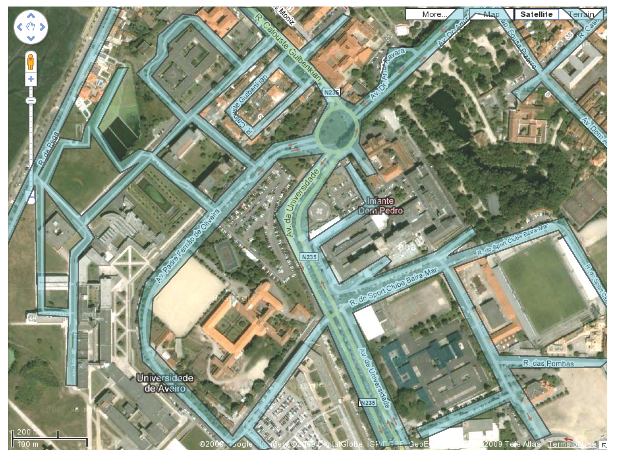
R be a polygonal region that models a street network (see
Figure 1, the background image was taken from Google Maps). People and vehicles can move within
R to reach specific locations there.
Figure 1.
The blue polygonal region models a street network.
Figure 1.
The blue polygonal region models a street network.
In this example, the set S of antennas is located at the buildings’ tops and not on the streets, so no antennas are found on R. However, the algorithms in this paper work for both cases. The regions within reach of at least two antennas are considered to be well covered. Therefore, the larger these regions the better the coverage of R. This restriction is derived by several real-life problems that may occur in situations where stronger monitoring is needed, such as military applications. This is also the case when multiple sensors are required to detect an event.
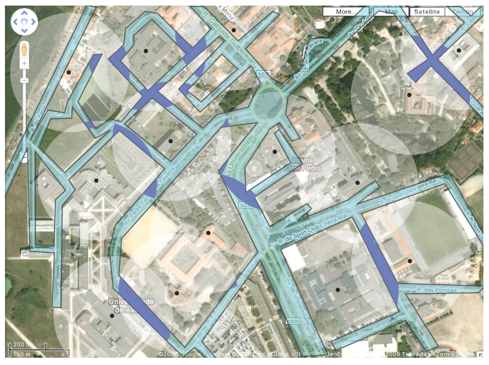
In
Figure 2 and
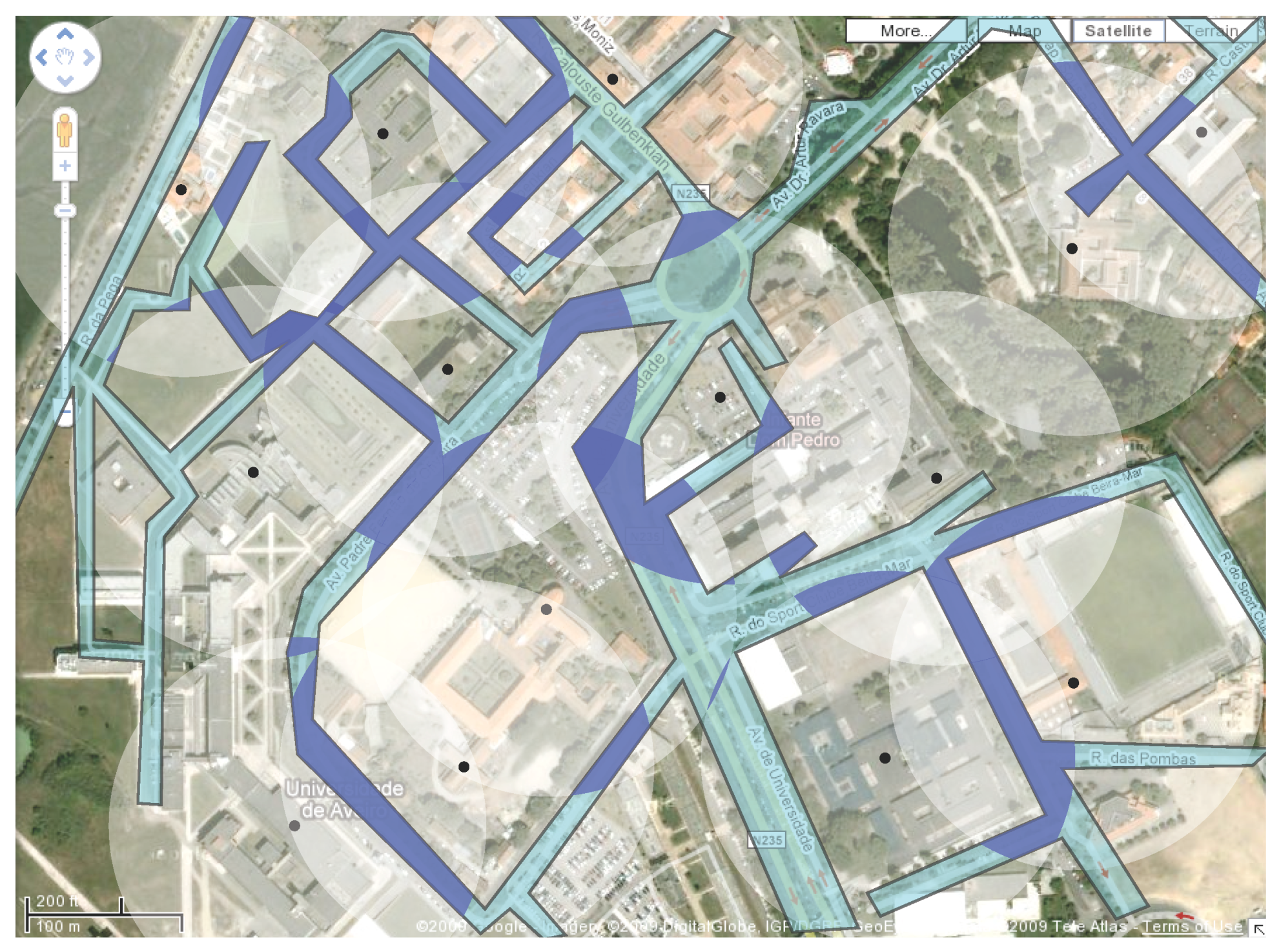
Figure 3 there are two examples of a polygonal region each with a set of homogeneous antennas (represented by black dots) whose coverage area is shown in white. The antennas’ range in
Figure 2 is shorter than in
Figure 3. The best covered regions, that is, regions that are within reach of at least two antennas are shown in dark blue. In these zones, any traffic would get a signal transmitted from at least two antennas.
Figure 2.
The areas of the polygonal region that are covered by at least two antennas are shown in dark blue.
Figure 2.
The areas of the polygonal region that are covered by at least two antennas are shown in dark blue.
Figure 3.
The areas of the polygonal region that are covered by at least two white antennas are shown in dark blue.
Figure 3.
The areas of the polygonal region that are covered by at least two white antennas are shown in dark blue.
As stated before, it can be seen that larger transmission ranges provide better coverage. However, as larger ranges also result in higher costs, it is appropriate to balance one against the other. Moreover, the optimisation of the antennas’ transmission range also improves the life span of wireless-enabled devices [
3]. Consequently, the main problem in this paper is to
minimise the antennas’ range in order to provide a good coverage of region R and or to assure the existence of a well covered path within R. What follows is therefore a formal definition of the problem. Assuming all distances are Euclidean, the distance between a point
q on the plane and a set
S of points is defined as the minimum distance between
q and any one point of
S. Point
q is said to be
covered by a set
S of antennas with power transmission range
r if the distance between
q and
S is less or equal to
r. Therefore, the antennas’ minimum transmission range that covers
q is the distance between
q and
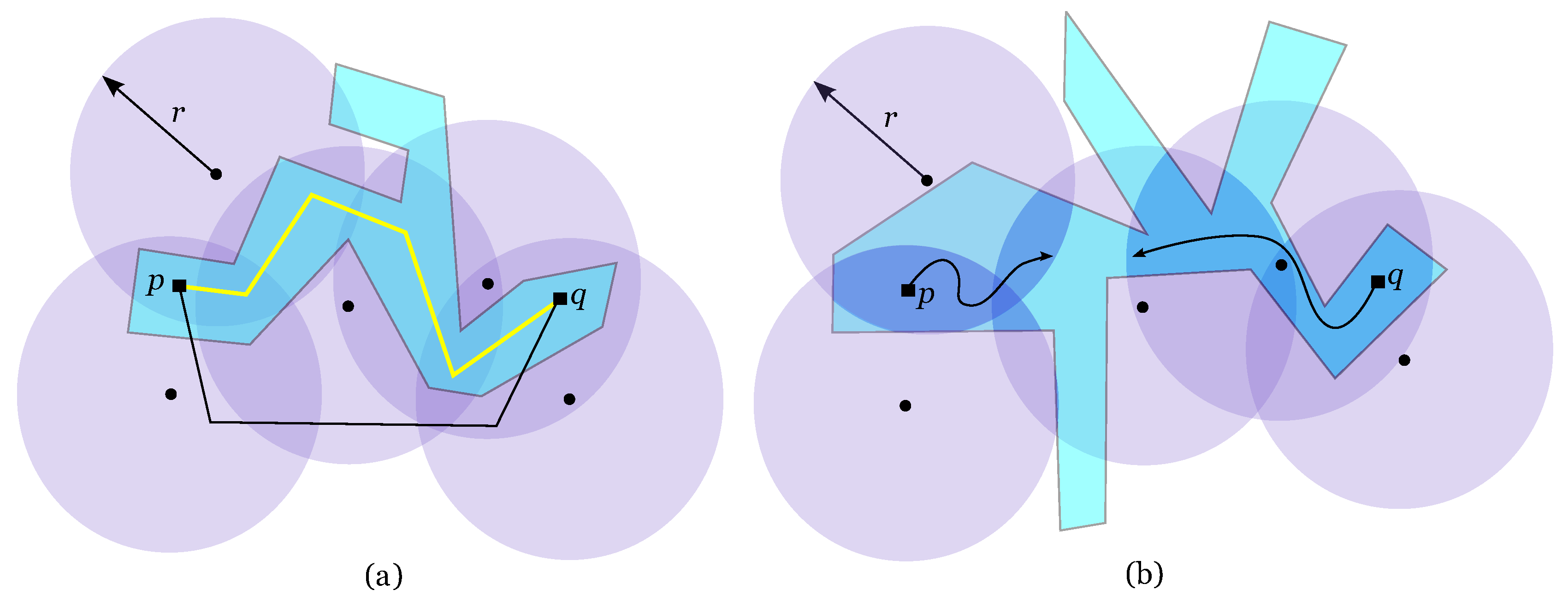
S. A point covered by two or more antennas of
S is said to be
2-covered by
S (see
Figure 4(a)). This definition aims towards quality coverage, as previously explained. The minimum power transmission range of
S that 2-covers an object
x is denoted by
. For example, if the object is a point
q,
is the minimum power transmission range of
S that 2-covers
q.
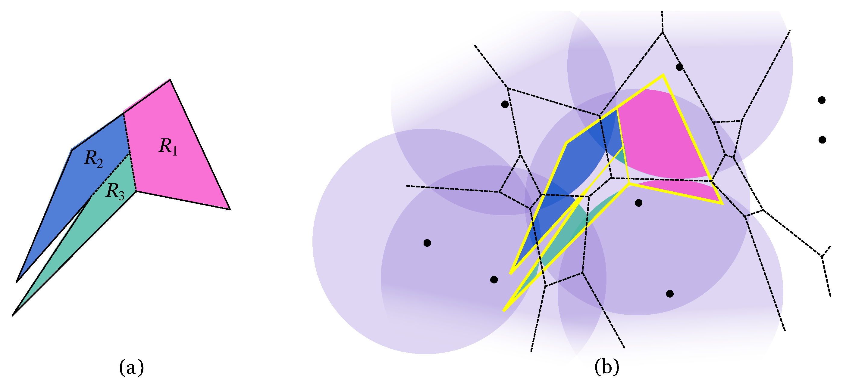
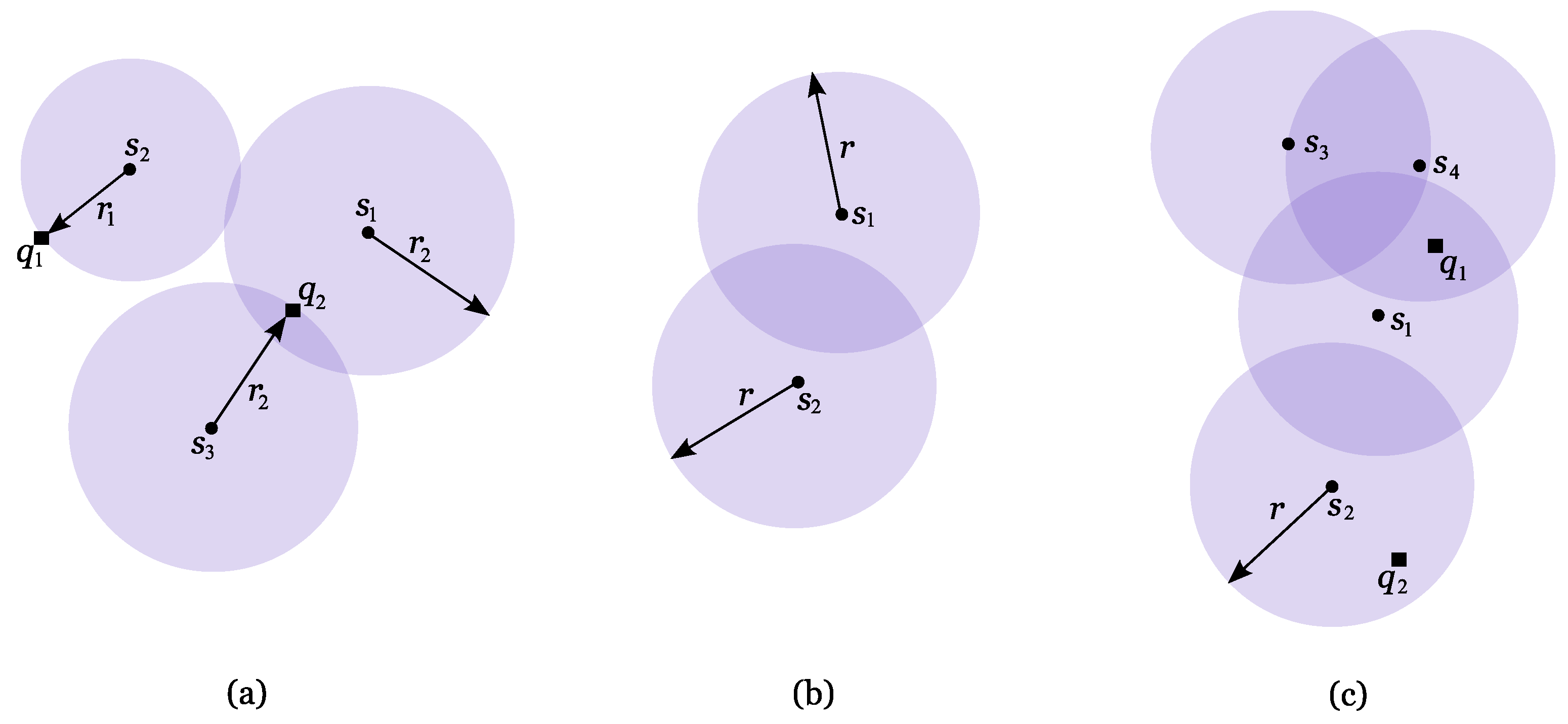
Figure 4.
Set S is represented by dots. (a) Point is covered by antenna with minimum range . Point is 2-covered by S with minimum range . (b) The lens formed by and is shown in dark purple. (c) Regions 2-covered by S with range r are shown in dark purple. Point is 2-covered by S, whilst is not.
Figure 4.
Set S is represented by dots. (a) Point is covered by antenna with minimum range . Point is 2-covered by S with minimum range . (b) The lens formed by and is shown in dark purple. (c) Regions 2-covered by S with range r are shown in dark purple. Point is 2-covered by S, whilst is not.
Let
be the set of discs of radius
r each centred at an antenna of
S. Each nonempty intersection between two discs of
D is called a
lens (see
Figure 4(b)). The union of these lenses encloses all the points on the plane that are 2-covered by
S, thus defining 2-
covered regions (see
Figure 4(c)). Every point within such regions clearly is 2-covered. The problems presented in the next sections aim to 2-cover a given region while minimising the antennas’ range
r. Note that the minimum range of the antennas that covers a point can be easily calculated in
time since such range is given by the distance between the point and its closest antenna. However, the Voronoi diagram of
S [
4] is a useful geometric structure that answers each query in
time. This diagram can be constructed in
time, so its construction is only justified when the number of queries regarding
S is larger than
. The two closest antennas to a given point can be found using the second order Voronoi diagram of
S, denoted by
. The second order Voronoi diagram of
S divides the plane into several regions by grouping points that share the same two closest antennas [
4]. It has the same complexity as the ordinary Voronoi diagram [
5]. This diagram is naturally related to the optimisation problems studied in this paper since a point is 2-covered if it is within range of its two closest antennas.
Following the previous terminology, there are several works related to geometric optimisation using 1-coverage. For example, Abellanas
et al. [
6] and Mehta
et al. [
7] study routes that are always close (or always far) to a given set of sensors on the plane. Agnetis
et al. [
8] compute a subset of a given set of discs with variable radii whose costs depend on their radii, as well as the same subset but with fixed costs to cover a given line segment at minimum cost. After Meguerdichian’s work [
1], others followed either by studying different versions of the coverage problem or by improving and proving previous results as are the cases of Boukerche
et al. [
2], Li
et al. [
9] and Mehta
et al. [
7]. Recently, Zhang
et al. [
10] developed two localised algorithms to identify whether a sensor is on the boundary of the area covered by a sensor network. In this work, one of the proposed algorithms is based on a technique called the localised Voronoi diagram and the other on neighbour embracing polygons. Contrary to some of the previous work, their algorithms can be applied to arbitrary topologies of the sensor network. Using variable radii sensors, Zhou
et al. [
11] address the problem of selecting a minimum energy-cost coverage, where each sensor can vary its sensing and transmission radius. They propose several centralised and distributed algorithms to compute a small subset sensors that are sufficient to cover the region required to be monitored. Das
et al. [
12] study efficient location of base stations to cover a convex region when the base stations are interior to the region. Making use of Voronoi diagrams, they developed a fast iterative algorithm to solve this problem. In their paper there are also some citations related to the coverage of a square or an equilateral triangle. Also employing Voronoi diagrams, Stoyan and Patsuk [
13] consider the problem of covering a compact polygonal set using identical discs of minimum radius. Boukerche
et al. [
2] address sensor networks by studying how well a large wireless sensor network can be monitored or tracked while keeping a long lifetime. Their solution outperforms previously known techniques. Bezdek and Kuperberg [
14] research an intermediate problem between 1-coverage and 2-coverage. They study the minimum coverage of the plane using homogeneous discs so that the region remains covered even when the radius of one of the discs decreases. This concept provides a continuous transition from 1-coverage to 2-coverage.
This paper is organised as follows: in
Section 2 it is shown how to minimise the power transmission range of a set
S of antennas to 2-cover a polygonal region
R (with or without holes). In
Section 3, it is introduced an algorithm to minimise the power transmission range that assures the existence of a 2-covered path between two points on
R. This problem is solved using the respective decision problem that is also addressed in this section. The cases where region
R is not polygonal are discussed in
Section 4, which is followed by a brief discussion of the results.
2. Minimum Transmission Range to 2-Cover a Polygonal Region
Let R be a polygonal region (with or without holes) and S a set of antennas with the same power transmission range. The boundary of R, denoted by , is considered to be part of the region R. Region R is said to be 2-covered by S if every point on R is 2-covered. The algorithm introduced in this section calculates the minimum power transmission range of S to 2-cover R, . Such range is calculated as being the largest distance between a point and its second closest antenna. Let the antennas’ range be large enough to 2-cover R. Now suppose this range is reduced until there is just one point that is no longer 2-covered. The antennas’ minimum range to 2-cover q is exactly . The following proposition characterises the location of point q on R.
Proposition 1 Let R be a polygonal region, q a point on R and S a set of antennas. If for some antenna ,
then q can only be one of the following:- (a)
A vertex of R;
- (b)
An intersection point between and ;
- (c)
A vertex of interior to R.
Proof:
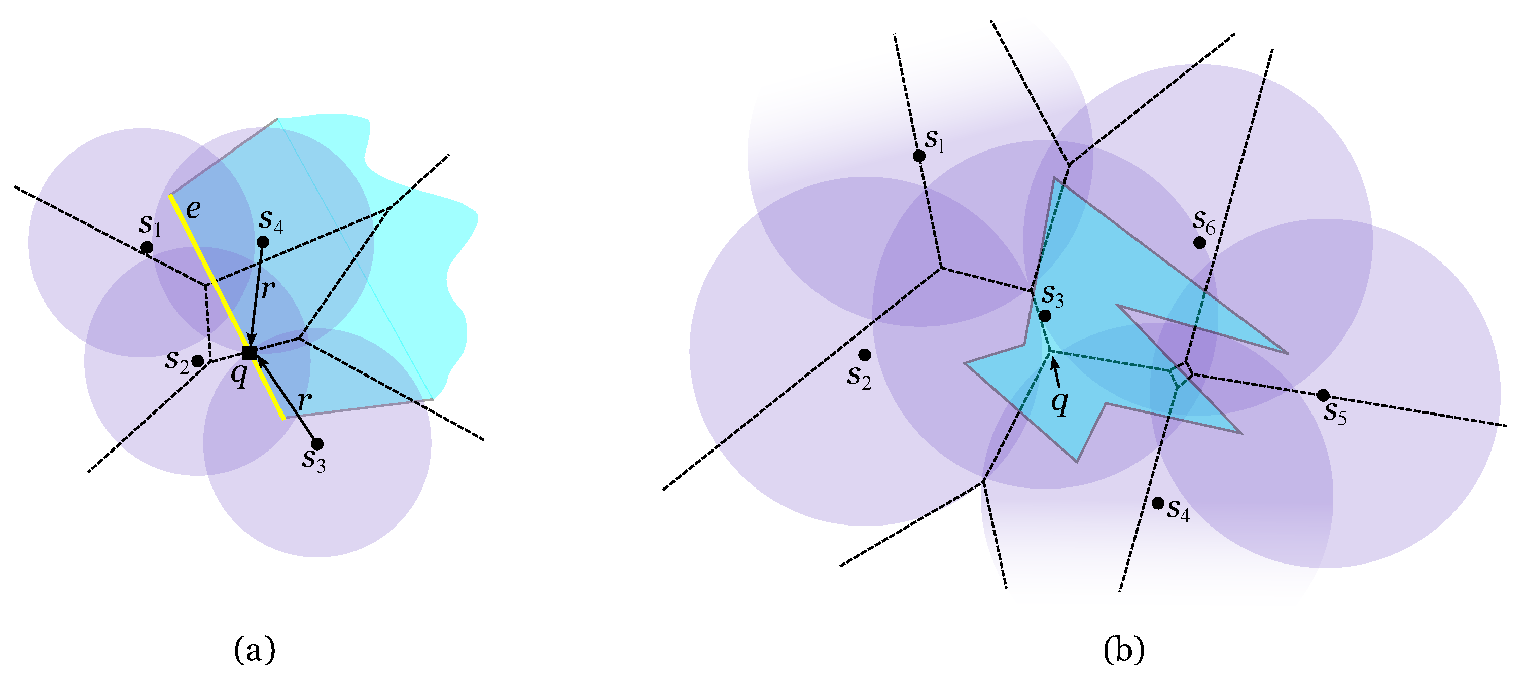
Let
be such that
for some antenna
. Given an edge
e of
R, it is easy to see that
is calculated using the intersection points between
e and
plus the endpoints of
e. The minimum range of
S that 2-covers all these points is exactly the minimum transmission range needed to 2-cover
e (see
Figure 5(a)). Consequently, if
then
q must be a vertex of
R or an intersection point between
and
. If
q is an interior point then the situation gets trickier since it does not depend on the shape of
R but on the way lenses interact with each other. As the antennas’ range increases, the lenses grow larger and fill the interior of
R. The last interior point to be 2-covered must be a point lying in the last “hole” (meaning a region of
R not yet 2-covered). These holes are filled when three lenses intersect at a time since not only the intersection point is 2-covered but also its whole neighbourhood (see
Figure 5(b)). Since three lenses intersect at a vertex of
[
15], if
q is interior to
R then it has to be a vertex of
.
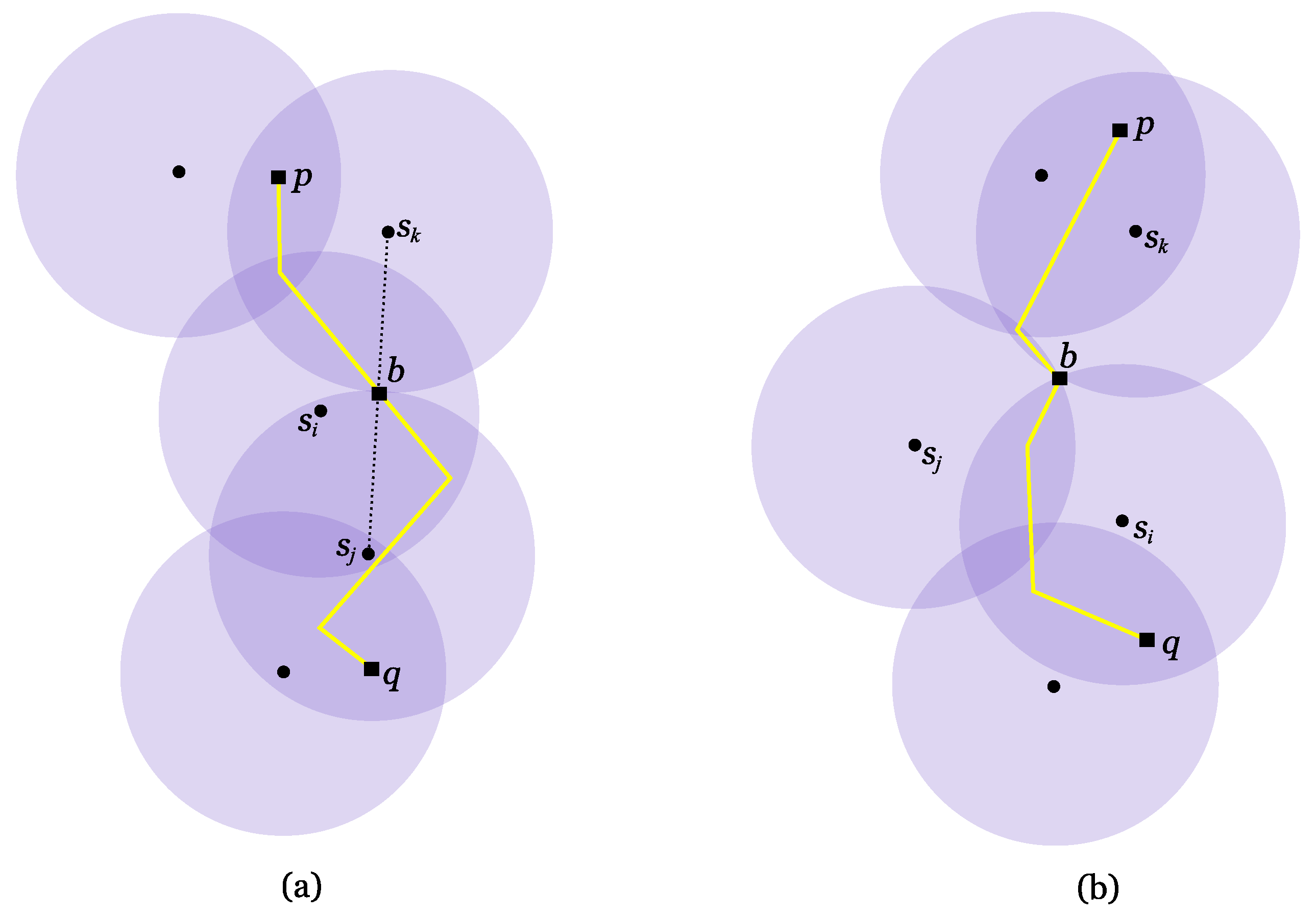
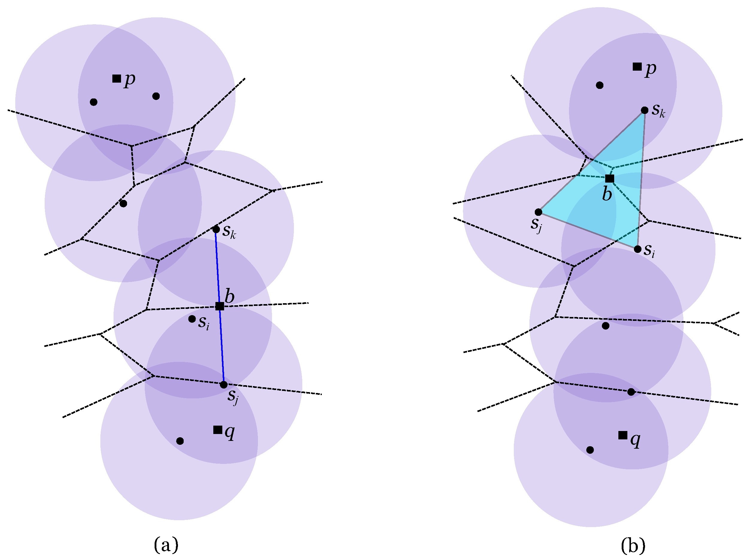
Figure 5.
(a) Line segment e is 2-covered with minimum range . (b) Point q is the last point to be 2-covered on R. It is a vertex of (shown in a dashed line).
Figure 5.
(a) Line segment e is 2-covered with minimum range . (b) Point q is the last point to be 2-covered on R. It is a vertex of (shown in a dashed line).
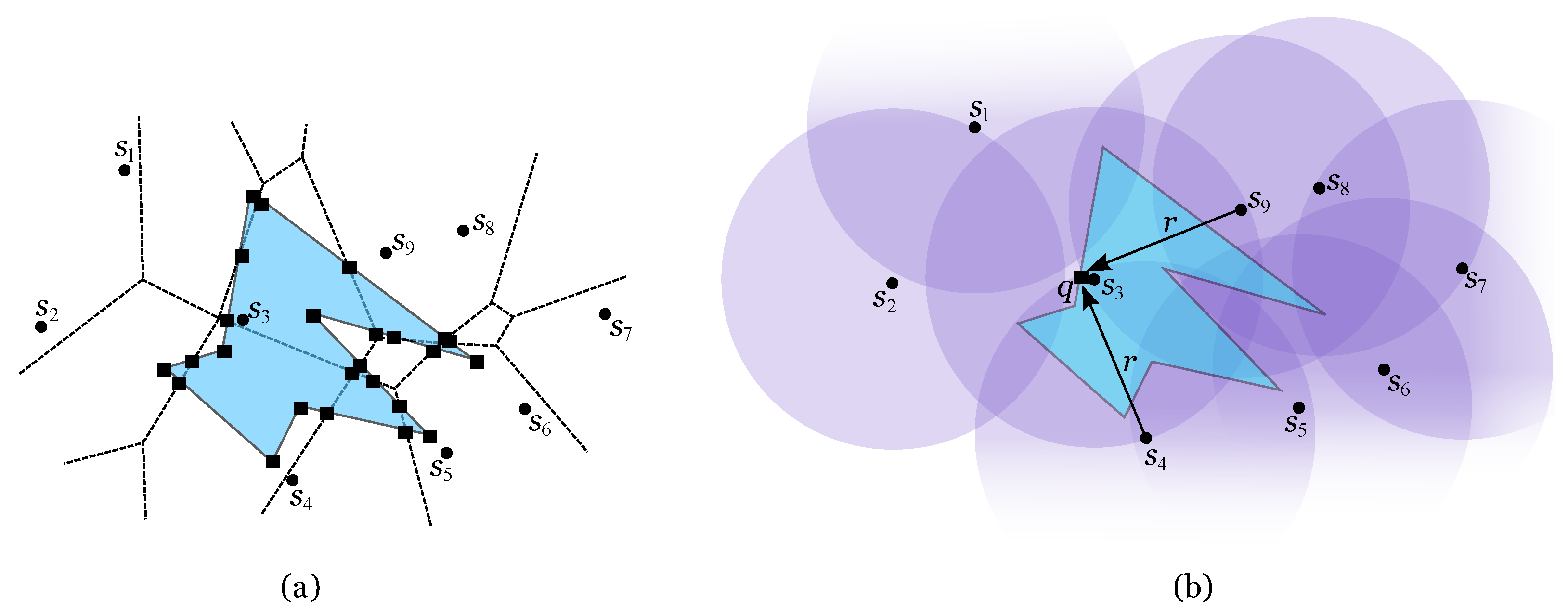
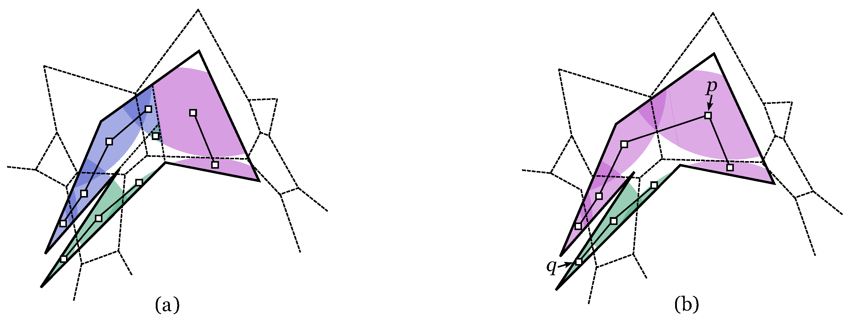
According to this proposition, there are several candidates on
R to be the point needing the largest range in order to be 2-covered. Since every point on
R has to be 2-covered,
is calculated as the minimum range to 2-cover every such candidate. Therefore, there is the need to analyse every vertex of
R, intersection points between
and
and vertices of
interior to
R (see
Figure 6(a)). In
Figure 6(b) there is an example of a 2-covered polygonal region
R with minimum power transmission range. The point of
R defining
is
and so
R is 2-covered if the antennas’ transmission range is at least
. The following algorithm calculates
.
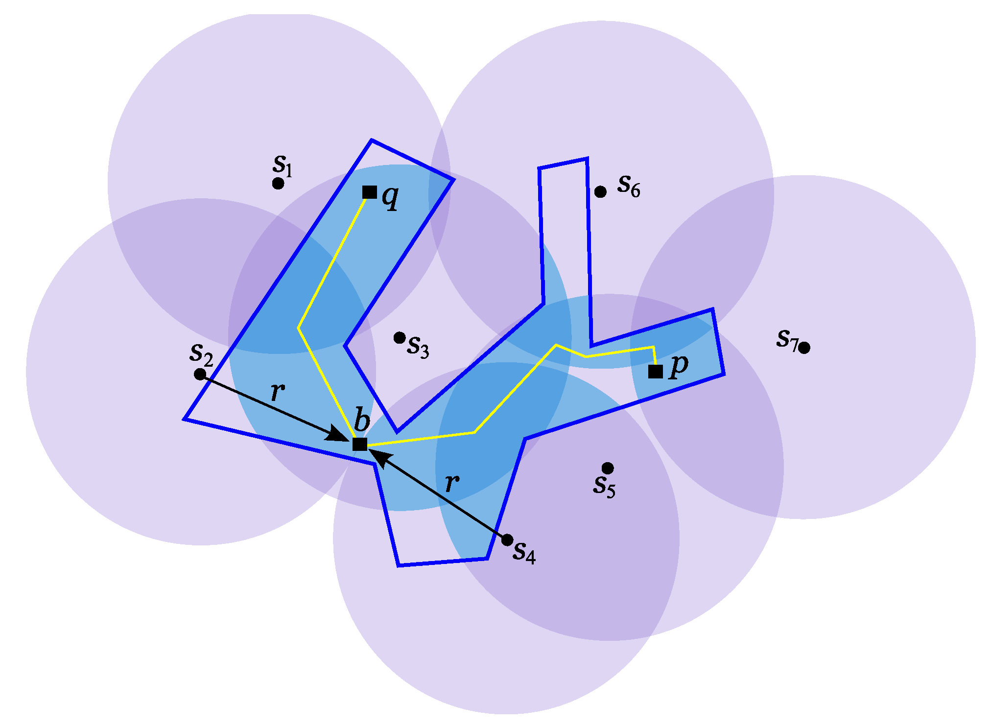
Figure 6.
(a) The candidates are represented by squares: vertices of R, points of and a vertex of interior to R. (b) .
Figure 6.
(a) The candidates are represented by squares: vertices of R, points of and a vertex of interior to R. (b) .
Algorithm Minimum Range to 2-Cover a Region
Input: Set S of n antennas and polygonal region R
Output:
1. Compute , the second order Voronoi diagram of S.
2. Compute the intersection set .
3. Add the vertices of that are interior to R to set I.
4. Add the vertices of R to set I.
5. .
The following result is a direct consequence of the algorithm Minimum Range to 2-Cover a Region.
Theorem 1 Given a set S of n antennas and a polygonal region R with m vertices, can be calculated in time and space.
Proof:
Computing
takes
time since
S is formed by
n antennas on the plane [
5]. The cardinality of set
is at most
since
has
n faces and
R has
m edges. Adding all the vertices of
that are interior to
R to set
I takes
time. The region’s vertices can be added to
I in
time. For each intersection point
,
is calculated in constant time using
as it is the distance between
q and its second closest antenna. The largest of these distances is
. Overall, the time complexity of this procedure is
. Regarding the space complexity, there is the need to store at most
intersection points while
can be stored in
space [
5]. Consequently, this algorithm runs in
time and space.
Corollary 1 Given a set S of n antennas and a convex polygonal region R with m vertices, can be calculated in time and space.
Note that, for a convex polygonal region R, can be calculated in time and space if has been previously built.
