Delaunay Meshing of Piecewise Smooth Complexes without Expensive Predicates

Abstract

Recently a Delaunay refinement algorithm has been proposed that can mesh piecewise smooth complexes which include polyhedra, smooth and piecewise smooth surfaces, and non-manifolds. However, this algorithm employs domain dependent numerical predicates, some of which could be computationally expensive and hard to implement. In this paper we develop a refinement strategy that eliminates these complicated domain dependent predicates. As a result we obtain a meshing algorithm that is practical and implementation-friendly.

1. Introduction

Delaunay mesh generation of non-smooth domains such as piecewise smooth surfaces and complexes is a difficult challenge. Aided by recent developments in sampling theory and computational topology, Chew’s furthest point strategy [1, 2] (Delaunay refinement) has been applied to generate Delaunay meshes for smooth surfaces with provable guarantees [3, 4]. The lack of global smoothness poses two main difficulties in extending these methods to non-smooth domains. First, the sampling theory developed for smooth surfaces breaks down for non-smooth surfaces. Secondly, small input angles possibly present at non-smooth regions pose problems for the termination of Delaunay refinement [5].

Boissonnat and Oudot [6] gave a provable algorithm for a class of non-smooth surfaces called Lipschitz-surfaces. They showed that their algorithm for smooth surface meshing [3] extends to this class only if input angles are sufficiently large. Unfortunately, this approach failed to admit small input angles which limited the input class. Rineau and Yvinec [7] implemented an algorithm for meshing volumes bounded by piecewise smooth surfaces; their approach also suffers from an angle constraint. Recently Cheng, Dey and Ramos [8] proposed an approach that completely removed any constraint on input angles. As a result their algorithm could accommodate large class of input domains called piecewise smooth complexes (PSCs). This class includes polyhedral domains, smooth and piecewise smooth surfaces, and even non-manifolds.

The algorithm of [8] uses the idea of protecting non-smooth curves and vertices in the input complex with balls. This idea already gave good results in the polyhedral case [9,10,11]. A novelty introduced by Cheng et al. is that they turn the balls into weighted points and then carry out the mesh refinement in the weighted Delaunay triangulation [12, 13]. Notwithstanding its theoretical success, practical relevance of this algorithm remains questionable. It employs some expensive numerical computations that are hard to implement. Unless these computations are removed, one cannot expect a practical solution for Delaunay mesh generation of PSCs. The goal of this paper is to design a refinement strategy without expensive predicates so that it becomes implementation-friendly and practical.

Bottleneck. Consider a smooth surface given by an implicit equation. To generate a meaningful mesh for this surface, one needs to sample it at a scale that captures its smallest local variations. One approach would be to guess a scale and sample the surface with it. If the guess is right, sampling with the furthest point strategy gives a mesh with provable guarantees as shown by Boissonnat and Oudot [3]. A second approach would be to compute a version of the local length scales and mesh the surface with those scales. The algorithm of Cheng et al. [8] works on this latter principle. It computes how a curve or a surface varies normal-wise around a point. It also computes separation distances between different elements (vertices, curves, and surfaces) to capture separation feature size (gap size) in the sense of [9, 14]. These assumed powerful numerical primitives allow Cheng et al. to determine the size of the protecting balls with certain desirable properties and allow them to sample surface patches at appropriate length scales. Unfortunately, these computations are expensive and are hard to implement which makes the algorithm impractical.

Solution. To circumvent the problem we follow the guessing approach. We would like to guarantee that even if the guess is incorrect, the algorithm terminates and outputs a mesh which approximates the input complex at a coarse level. A main difficulty in this approach is to formulate a unified refinement strategy that captures the input topology correctly when the guessed scale is right and outputs a mesh with some reasonable properties all the time. To reach this goal we formulate a disk condition that says that the output mesh should have a topological disk formed by triangles around each vertex. This disk condition drives the refinement, that is, we go on refining protecting balls or surface meshes if this disk condition fails. If this refinement terminates, the disk condition necessarily holds for the output mesh. Then, by PL topology, the output Delaunay mesh restricted to each manifold surface patch is a manifold. Furthermore, the input incidence structure among different elements in the PSC is maintained. The output may not be homeomorphic to the input since a small feature such as a small handle may not be detected at the length scale the algorithm is asked to operate. However, a homeomorphic meshing is guaranteed when the supplied scale is sufficiently small. Actually, in practice, the disk condition usually suffices to provide a homeomorphism.

One of our main tasks is to prove that the refinement always terminates. To this end we use the following result. If the protecting balls are sufficiently small and satisfy some separation properties (conditions C1-C3 in Section 2.), then the disk condition holds if the restricted Delaunay triangles are sufficiently small. Therefore, the failure of the disk condition signals either balls do not satisfy separation properties, or are large, or triangles are large. The way we compute the protecting balls, failure of separation properties also implies that they are large. In essence, if the disk condition fails, either a ball or a triangle is too large. The algorithm refines the larger of the two and hence guarantees that neither a protecting ball nor a triangle gets arbitrarily small ensuring termination. One may observe that, this strategy does not allow adaptive mesh sizing. However, one may regulate the input scale to produce meshes at different levels of resolution.

Perhaps the most important ingredient in this approach is to maintain a set of protecting balls with the separation properties. It turns out that it is difficult to ensure one of these properties exactly (condition C3) when the balls are large. Instead we maintain a more relaxed condition which implies the desired property when the balls are sufficiently small.

We have implemented our algorithm in this paper. In an earlier attempt we tried to mesh with the disk condition but pre-computed the balls with a small radius chosen heuristically [15]. The code failed in cases where the pre-selected size of the balls was wrong. The approach in this paper allows the refinement algorithm to determine the balls automatically instead of pre-computing them. We report experimental results for our protection algorithm and meshing in Section 5. The code and a video explaining the experimental results have been released [16].

1.1. Domain

Throughout this paper, we assume a generic intersection property that a k-manifold $\sigma \subset {\mathbb{R}}^3$, $0⩽k⩽2$, and a j-manifold ${\sigma }^{\prime }\subset {\mathbb{R}}^3$, $0⩽j⩽2$, intersect (if at all) in a $(k+j-3)$-manifold if $\sigma \neg \subset {\sigma }^{\prime }$ and ${\sigma }^{\prime }\neg \subset \sigma$. We will use both geometric and topological versions of closed balls. A geometric closed ball centered at point $x\in {\mathbb{R}}^3$ with radius $r>0$, is denoted as $B(x,r)$. We use $\mathrm{int}\mathbb{X}$ and $\mathrm{bd}\mathbb{X}$ to denote the interior and boundary of a topological space $\mathbb{X}$, respectively.

The domain D is a piecewise smooth complex (PSC) where each element is a compact subset of a smooth ($C^2$) k-manifold, $0⩽k⩽2$. Each element is closed and hence contains its boundaries. For simplicity we assume that each element has a non-empty boundary (used in Lemma 8, this restriction can be removed by some added complication in the initialization of the algorithm). We use $D_k$ to denote the subset of all k-dimensional elements, the kth stratum. $D_0$ is a set of vertices; $D_1$ is a set of curves called 1-faces; $D_2$ is a set of surface patches called 2-faces. For $1⩽k⩽2$, we use $D_{⩽k}$ to denote $D_0\cup \dots \cup D_k$.

The domain D satisfies the usual proper requirements for being a complex: (i) interiors of the elements are pairwise disjoint and for any $\sigma \in D$, $\mathrm{bd}\sigma \subset D$; (ii) for any $\sigma ,{\sigma }^{\prime }\in D$, either $\sigma \cap {\sigma }^{\prime }=\varnothing$ or $\sigma \cap {\sigma }^{\prime }$ is a union of elements in D. We use $|D|$ to denote the underlying space of D. For $0⩽k⩽2$, we also use $|D_k|$ to denote the underlying space of $D_k$.

1.2. Complexes

We will be dealing with weighted points and their Delaunay and Voronoi diagrams. A weighted point p with weight ${\omega }_p$ is represented as a ball $b=B(p,{\omega }_p)$. The squared weighted distance of any two points p and q is $\widehat{d}{(p,q)}^2=d{(p,q)}^2-{\omega }_p^2-{\omega }_q^2$ where ${\omega }_p$ and ${\omega }_q$ are the weights of p and q respectively. With this definition, an unweighted point $x\in {\mathbb{R}}^3$ has a distance of $\widehat{d}(x,p)=\sqrt{d{(x,p)}^2-{\omega }_p^2}$ from p. Under the distance metric $\widehat{d}(·,·)$, one can define weighted versions of Delaunay and Voronoi diagrams. For a weighted point set $S\subset {\mathbb{R}}^3$, let $\mathrm{Vor}S$ and $\mathrm{Del}S$ denote the weighted Voronoi and Delaunay diagrams of S respectively. Each diagram is a cell complex where each k-face is a k-polytope in $\mathrm{Vor}S$ and is a k-simplex in $\mathrm{Del}S$. Each k-simplex ξ in $\mathrm{Del}S$ is dual to a $(3-k)$-face $V_{\xi }$ in $\mathrm{Vor}S$ and vice versa.

Let S be a point set sampled from $|D|$. For any sub-collection $\mathbb{X}\subset D$ we define ${\mathrm{Del}S|}_{\mathbb{X}}$ to be the Delaunay subcomplex restricted to $\mathbb{X}$, i.e., each simplex ${\xi \in \mathrm{Del}S|}_{\mathbb{X}}$, called a restricted simplex, is the dual of a Voronoi face $V_{\xi }$ where $V_{\xi }{|}_{\mathbb{X}}=V_{\xi }\cap |\mathbb{X}|\ne \varnothing$. By this definition, for any $\sigma \in D$, ${\mathrm{Del}S|}_{\sigma }$ denotes the Delaunay subcomplex restricted to σ, and ${\mathrm{Del}S|}_{D_i}={\bigcup }_{\sigma \in D_i}{\mathrm{Del}S|}_{\sigma }and\mathrm{Del}S{{|}_D={\bigcup }_{\sigma \in D}\mathrm{Del}S|}_{\sigma }.$ An i-face $\sigma \in D_i$ should be meshed with i-simplices. However, ${\mathrm{Del}S|}_{\sigma }$ may have lower dimensional simplices not incident to any restricted i-simplex. Therefore, we compute special sub-complexes of restricted complexes. Define the following i-dimensional subcomplexes (see Figure 1):

$${\mathrm{Skl}}^i{S|}_{\sigma }={\{t|t\in \mathrm{Del}S|}_{\sigma }$$

is an i-simplex or a sub-simplex of an i-simplexand

$${\mathrm{Skl}}^{i}S{{|}_{D_i}=\bigcup _{\sigma \in D_i}{\mathrm{Skl}}^{i}S|}_{\sigma }.$$

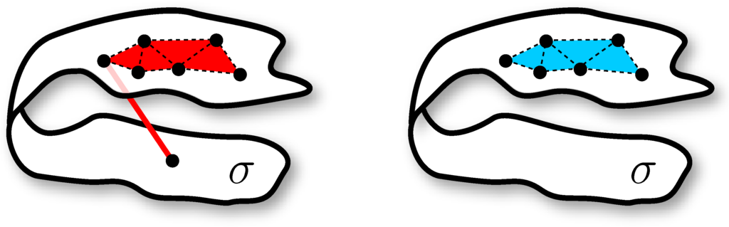
Figure 1. (left) ${\mathrm{Del}S|}_{\sigma }$ and (right) ${\mathrm{Skl}}^2{S|}_{\sigma }$ There is one extra edge in ${\mathrm{Del}S|}_{\sigma }$ which is not in ${\mathrm{Skl}}^2{S|}_{\sigma }$.

2. Protection and Refinement

The meshing algorithm computes a set of balls protecting 1-faces. Unlike [8], the protecting balls are adjusted on the fly as refinement proceeds. It inserts points in 2-faces to refine the triangulation. The protecting balls and the triangulation are refined simultaneously either to satisfy a disk condition or to achieve a refinement level dictated by an input scale parameter. In what follows all skipped proofs appear in the appendix.

2.1. Covering 1-faces

Let $\sigma (x,y)$ denote the curve segment oriented from x to y on any 1-face σ. In this notation $\sigma =\sigma (u,v)$ where σ is oriented from the end point u to the other end point v. Let $b=B(c,r)$ be a ball with $c\in \sigma (x,y)$. The intersection $b\cap \sigma$ is a set of curve segments. Among them the curve segment containing c is called the segment of b in σ, ${\mathrm{seg}}_{\sigma }\left(b\right)$, see Figure 2. Two balls b and $b^{\prime }$ with their centers c and $c^{\prime }$ respectively on a 1-face σ are adjacent if $\sigma (c,c^{\prime })$ does not contain any other ball center. In this case the corresponding weighted vertices of b and $b^{\prime }$ are also called adjacent. Any two balls or weighted vertices that are not adjacent are called non-adjacent. We use $d(x,y)$ to denote the Euclidean distance between two points $x,y$ and use $d_{\sigma }(x,y)$ to denote the length of a curve segment $\sigma (x,y)$. Let $b_0,b_1,...,b_k$ be a set of balls that protect σ where $b_i=B(c_i,r_i)$ with $c_i\in \sigma$. We require that the balls satisfy the following conditions:

(C1)

$b_0$ and $b_k$ are centered at u and v respectively. These will be called the vertex balls.

(C2)

σ is covered by the balls, that is, $\sigma \subseteq {\cup }_i{\mathrm{seg}}_{\sigma }\left(b_i\right)$ and any two adjacent balls $b=B(c,r)$ and $b^{\prime }=B(c^{\prime },r^{\prime })$ intersect deeply, that is, $d(c,c^{\prime })⩽r+\frac{6r^{\prime }}{7}$ where $r^{\prime }⩽r$.

(C3)

No point in ${\mathrm{seg}}_{\sigma }\left(b_i\right)$ is contained in a ball non-adjacent to $b_i$.

Notice that the choice of the constant $\frac{6}{7}$ in C2 is a little arbitrary. We need only a factor of $r^{\prime }$ in the expression and a follow-up analysis with other constants are also possible.

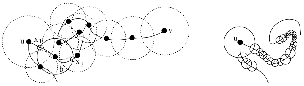
Figure 2. Covering 1-faces : (left) A 1-face σ between u and v is being protected. The ball b shown with solid boundary has ${\mathrm{seg}}_{\sigma }\left(b\right)$ as the curve segment between $x_1$ and $x_2$. The balls satisfy C1 and C2 but intersect arbitrarily. (right) Balls are refined and they start satisfying separation properties C1-C3.

We will maintain a point set $S\subset D$ with the following properties throughout the algorithm: all points in S except those in $D_{⩽1}$ are unweighted and no unweighted point has a negative weighted distance to any other point. This means each unweighted point $p\in S$ has $V_p$ non-empty. We call such a point set admissible.

It is worthwhile to note that one of the consequences of conditions C1-C3 would be the following result which would imply R2 in Lemma 2.

Lemma 1 Let S be an admissible point set satisfying conditions C1-C3. Let p and q be adjacent weighted vertices on a 1-face σ. $V_{pq}$ is the only Voronoi facet in $\mathrm{Vor}S$ that intersects $\sigma (p,q)$.

Let z be any point in $\sigma (p,q)$. Let $b_p$ and $b_q$ be the balls centered at p and q respectively. The point z is contained in $b_p\cup b_q$. Due to property C3, z being a point in $\sigma (p,q)$ cannot lie inside any ball other than $b_p$ and $b_q$. We remark that $b_p$ and $b_q$ may have a common intersection with another ball, but z cannot be contained in that ball. Therefore, z cannot lie on any Voronoi facet partly defined by a point other than p and q. However, $\sigma (p,q)$ has to intersect at least one Voronoi facet since p and q lie in two different Voronoi cells. Therefore, the only Voronoi facet which intersects $\sigma (p,q)$ is $V_{pq}$.

For any $\sigma \in D_2$ and any triangle $t\in {\mathrm{Skl}}^2{S|}_{\sigma }$, define $\mathrm{size}(t,\sigma )$ to be the maximum weighted distance between the vertices of t and points in $V_t{|}_{\sigma }$. This is the maximum weighted distance between vertices of t and the points where the dual Voronoi edge of t intersects σ.

λ-property: We say S has the λ-weight property if each point in S has a weight at most $\lambda ⩾0$. We say S has the λ-size property if $\mathrm{size}(t,\sigma )⩽\lambda$ for each triangle $t\in {\mathrm{Skl}}^2{S|}_{\sigma }$ and S has the λ-weight property.

The following observation is at the heart of our refinement algorithm (see Section 7. in appendix for a proof sketch).

Lemma 2 Let $S\subset D$ be an admissible point set and $p\in S$ be a point on a 2-face σ. Let ${\sigma }_p\subset \sigma$ be the set of all connected components in $V_p{|}_{\sigma }$ that intersect a Voronoi edge. There exists a constant $\lambda >0$ so that hypotheses H1 and H2 imply results R1 and R2 where

(H1)

S satisfies λ-size property.

(H2)

Weighted points in S satisfy C1-C3.

(R1)

${\sigma }_p$ is a 2-disk where any edge of $V_p$ intersects ${\sigma }_p$ at most once and any facet of $V_p$ intersects ${\sigma }_p$ in an empty set or an open curve.

(R2)

If $p\in \mathrm{bd}\sigma$, at least two Voronoi facets of $V_p$ intersect $\mathrm{bd}\sigma$, each intersecting one of the curve segments between p and its adjacent weighted points (possibly two) in $\mathrm{bd}\sigma$.

Interpreted in terms of the Delaunay triangulation, the conclusion of the above lemma implies that the triangles incident to p and restricted with respect to σ form a topological disk around p. This disk has p at the boundary if and only if p is in $\mathrm{bd}\sigma$. Furthermore, if p is in $\mathrm{bd}\sigma$, it is connected to its two adjacent weighted points in $\mathrm{bd}\sigma$ on this disk. We will formulate a disk condition with these properties. Our refinement algorithm is primarily driven by this disk condition. The conclusion of Lemma 2 fails only if either there is a protecting ball with radius more than λ, or there is a triangle $t\in {\mathrm{Skl}}^2{S|}_{\sigma }$ for which $\mathrm{size}(t,\sigma )>\lambda$ for some $\lambda >0$. However, since we do not know which of the above two cases has happened, we take a conservative approach. We compute the maximum radius $r_{max}$ of all protecting balls and also compute the maximum $d_{max}=\mathrm{size}(t,\sigma )$ over all t and σ. Let x be the point of intersection of a Voronoi edge with D which realizes $d_{max}$. If $r_{max}>d_{max}$ we refine the largest protecting ball. Otherwise, we insert x. In the first case we are ensured that we are refining balls of size larger than a fixed positive constant. In the second case, we are inserting a point in a compact domain with a positive lower bound on its distances to every other points. Termination by packing argument follows.

For the above algorithm to work, it is important that the balls satisfy C1-C3 when balls are sufficiently small. It turns out that it is difficult to maintain the condition C3 at early phases when the balls are relatively large. We replace C3 by the following two conditions that are maintained by the ball refinement algorithm. These conditions imply C3 when the balls are small enough. For a 1-face $\sigma (u,v)$ covered by balls $b_0,b_1,..,b_k$ these conditions are:

(C3.a)

Let $b=B(c,r)$ be any ball in $\{b_0,b_1,...,b_k\}$. For an adjacent ball $b^{\prime }=B(c^{\prime },r^{\prime })$, if $c^{\prime }$ is contained in ${\mathrm{seg}}_{\sigma }\left(b\right)$, then $d_{\sigma }(c,c^{\prime })⩾\frac{7}{6}r$.

(C3.b)

Any two balls centered in different 1-faces do not intersect and any two non-adjacent balls centered on a common 1-face have a weighted distance larger than the radius of the smaller ball.

Lemma 3 There exists a $\lambda >0$ so that, if all protecting balls are smaller than λ, C3.a and C3.b imply C3.

Consider any two non-adjacent balls $b=B(c,r)$ and $b^{\prime }=B(c^{\prime },r^{\prime })$. If c and $c^{\prime }$ are on different 1-faces, b and $b^{\prime }$ do not intersect by C3.b. Then C3 is satisfied trivially. So, assume that c and $c^{\prime }$ belong to a common 1-face σ.

We show that ${\mathrm{seg}}_{\sigma }\left(b\right)$ and ${\mathrm{seg}}_{\sigma }\left(b^{\prime }\right)$ do not intersect for sufficiently small λ. It follows from the differentiability of σ that there exists a $\lambda >0$ so that any ball of size smaller than λ intersects σ in a single segment. Assuming that b and $b^{\prime }$ have radii smaller than λ, we have $b\cap \sigma ={\mathrm{seg}}_{\sigma }\left(b\right)$ and $b^{\prime }\cap \sigma ={\mathrm{seg}}_{\sigma }\left(b^{\prime }\right)$. We claim that no point in ${\mathrm{seg}}_{\sigma }\left(b^{\prime }\right)$ can lie in ${\mathrm{seg}}_{\sigma }\left(b\right)$ when λ is sufficiently small. If there were such a point, there would exists a ball $b^{\prime \prime }$ with one of the following properties: (i) either $b^{\prime \prime }$ is adjacent to b and its center $c^{\prime \prime }$ lies in ${\mathrm{seg}}_{\sigma }\left(b\right)$, or (ii) $b^{\prime \prime }$ is adjacent to $b^{\prime }$ and $c^{\prime \prime }$ lies in ${\mathrm{seg}}_{\sigma }\left(b^{\prime }\right)$. Without loss of generality, assume that (i) holds since the other case can be argued exactly the same way.

We know that the length $d_{\sigma }(c,c^{\prime \prime })$ is at least $\frac{7}{6}r$ by property C3.a. Making λ sufficiently small, $d(c,c^{\prime \prime })$ can be set arbitrarily close to $d_{\sigma }(c,c^{\prime \prime })$ which would imply that $d_{\sigma }(c,c^{\prime \prime })$ can be made arbitrarily close to r. This would contradict that $d_{\sigma }(c,c^{\prime \prime })$ is at least $\frac{7}{6}r$. Therefore, we can claim that the curve segments of two non-adjacent balls cannot intersect if they are centered on a same 1-face σ.

2.2. Ball refinement

The ball refinement routine simply removes a ball and covers the curve segment between the centers of its adjacent balls with balls of smaller radii. Therefore, we encounter the generic situation where a curve segment $\sigma (x,y)$ needs to be covered by protecting balls whose radii are determined by a given parameter $\alpha >0$. The points x and y are the right and left end points of some segments, say ${\mathrm{seg}}_{\sigma }\left(b_0\right)$ and ${\mathrm{seg}}_{\sigma }\left(b_k\right)$ respectively, see Figure 3. We call this routine Cover($x,y,\alpha$).

We proceed from x toward y along the curve while computing the balls that satisfy conditions C1, C2, and C3.a. Condition C3.b is taken care of by another routine called Separate. As we walk from x to y, each step places a new ball of radius α that intersects deeply with the previous ball while covering a new piece of the curve. When we reach y, we place a ball that intersects deeply with both the endpoint ball and the previous one in the walk.

More specifically, suppose that $b_i=B(c_i,r_i)$ is already computed. Let $\sigma (x_i,y_i)={\mathrm{seg}}_{\sigma }\left(b_i\right)$. We compute a small ball ${\beta }_{i+1}=B(y_i,\alpha /3)$ that aids the computation of $b_{i+1}$, see Figure 3. The aiding ball helps compute the next ball so that its center is not contained in the segment of the previous ball. Among the two end points of segment ${\mathrm{seg}}_{\sigma }\left({\beta }_{i+1}\right)$, we use the one which is further from x. Let this end point be $z_{i+1}$. The center of the next ball $b_{i+1}$ is placed at $z_{i+1}$.

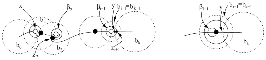
Figure 3. Curve segment between x and y is being covered. Aiding balls are shown with solid boundaries. Notice how the centers of $b_1$ and $b_2$ are placed with the aiding balls. The end game with enlarged aiding ball is shown on left, the other case is shown on right.

We will eventually encounter one of two situations near the end: either $z_{i+1}$ extends past $\sigma (x,y)$ or ${\mathrm{seg}}_{\sigma }\left(b_{i+1}\right)$ contains y. These situations are shown in the left and right images of Figure 3, respectively. In the first case $b_k$ may violate C3.a and in the second case $b_{i+1}$ may not intersect $b_k$ deeply violating C2. In these cases we conduct an end game. If $z_{i+1}\in {\mathrm{seg}}_{\sigma }\left(b_k\right)$, we throw away $z_{i+1}$ and take $b_{i+1}$ as ${\beta }_{i+1}$ enlarged concentrically to a radius $\frac{2\alpha }{3}$. In the other case when ${\mathrm{seg}}_{\sigma }\left(b_{i+1}\right)$ contains y, we enlarge $b_{i+1}$ to a radius of $\frac{7\alpha }{6}$. Cover terminates after the end game. Lemma 4 is proved in the appendix.

Lemma 4 Let b be a ball adjacent to $b^{\prime }$ and $b^{\prime \prime }$ in a set of balls that satisfy C1, C2, and C3.a. Suppose we replace b with Cover $(x,y,\alpha )$ where $\sigma (x,y)$ is the segment between ${\mathrm{seg}}_{\sigma }\left(b\right)$ and ${\mathrm{seg}}_{\sigma }\left(b^{\prime \prime }\right)$. Then, for α less than the radii of the balls $b,b^{\prime }$, and $b^{\prime \prime }$, C1, C2, and C3.a remain satisfied after Cover $(x,y,\alpha )$ terminates.

Cover does not necessarily satisfy C3.b. We use the routine Separate to enforce C3.b on a set of balls $\mathcal{B}$. This routine calls RefineBall(b) which removes the ball b and replaces it with smaller balls.

Separate($\mathcal{B}$)

while (∃ balls $b,b^{\prime }\in \mathcal{B}$ with $r⩾r^{\prime }$ violating C3.b)

$\mathcal{B}:=(\mathcal{B}\setminus b)\cup$ RefineBall (b)

endwhile.

2 return $\mathcal{B}$.

Lemma 5 If Separate issues a call to refine a ball b, its radius must be more than a fixed positive constant $\delta >0$.

First assume that the two balls $b=B(c,r)$ and $b^{\prime }=B(c^{\prime },r^{\prime })$ considered by Separate belong to the same 1-face σ. By assumption $r⩾r^{\prime }$. Let x be any point where the boundary spheres of b and $b^{\prime }$ meet. If θ is the angle between the normals to b and $b^{\prime }$ at x, the squared weighted distance between b and $b^{\prime }$ is given by $d{(c,c^{\prime })}^2-r^2-r^{\prime 2}=-2r{r}^{\prime }cos\theta$. For $\pi /2<\theta ⩽\pi$, this weighted distance is more than $r^{\prime }$ when $r>-r^{\prime }/2cos\theta$ which is satisfied for $\theta >2\pi /3$. The curve $\sigma (c,c^{\prime })$ can be assumed to lie within cones having apexes at c and $c^{\prime }$ and arbitrarily small aperture angles if r and hence $d(c,c^{\prime })$ is sufficiently small. Since ${\mathrm{seg}}_{\sigma }\left(b\right)$ and ${\mathrm{seg}}_{\sigma }\left(b^{\prime }\right)$ do not intersect if r is small enough (Proof of Lemma 3), the curve $\sigma (c,c^{\prime })$ needs to avoid the common intersection of b and $b^{\prime }$. These two constraints force the angle θ to be close to π as r approaches zero. In other words, there is a fixed positive constant ${\lambda }_1$ so that if $r⩽{\lambda }_1$, the weighted distance between b and $b^{\prime }$ becomes larger than $r^{\prime }$.

Next, assume that b and $b^{\prime }$ have centers on different 1-faces. We need to consider the special case of vertex balls before we argue about this case. A vertex ball b can intersect a ball whose center lies on a different 1-face only if b’s radius is more than a fixed positive constant. This is true because we always refine the larger of the two such intersecting balls and there is a positive distance between a vertex and any 1-faces that do not contain it. This observation with the argument in the previous paragraph imply that a vertex ball is refined by Separate only if its size is more than a fixed positive constant. Since no vertex balls can be smaller than a fixed positive constant, two balls centered on two different 1-faces intersect only if the larger ball has a radius more than a fixed positive constant ${\lambda }_2>0$.

It follows that the lemma holds with $\delta =min\{{\lambda }_1,{\lambda }_2\}$.

RefineBall(b)

If b covers $\sigma \in D_1$, let $r_{\sigma }$ be the minimum of the radii of balls adjacent to b on σ and b itself.

If $b=B(v,r)$ is a vertex ball, shrink b to $b^{\prime }=B(v,r/2)$. For each σ covered by b let $b_{\sigma }$ be the adjacent ball to b on σ. Compute ${\mathcal{B}}_{\sigma }$ := RefineBall $\left(b_{\sigma }\right)$. Return Separate(${\cup }_{\sigma }{\mathcal{B}}_{\sigma }$). If b is not a vertex ball, let $\sigma (x,y)$ be the segment between ${\mathrm{seg}}_{\sigma }\left(b_1\right)$ and ${\mathrm{seg}}_{\sigma }\left(b_2\right)$ where $b_1$ and $b_2$ are adjacent to b. Remove b and return Cover$(x,y,\alpha )$ where $\alpha =r_{\sigma }/4$.

Lemma 6 (i) RefineBall terminates and (ii) maintains C1, C2, C3.a, and C3.b.

(i) : Observe that RefineBall makes recursive calls to itself and through Separate. Consider the trees of ball refinements made by these recursive calls. An internal node b in the trees represents a ball b that is refined into smaller balls (children).

We observe that every internal node except the roots is refined by Separate. The only way RefineBall can call itself is when a ball $b_{\sigma }$ is to be refined in step 1. But, then $b_{\sigma }$ becomes a root. All other calls to RefineBall are generated by Separate.

By Lemma 5, Separate calls RefineBall on a ball b only if the size of b is larger than a fixed positive constant $\delta >0$. The children of a node b are created by Cover which, by construction, creates only finitely many balls with radius at most $(1/4\times 7/6)=7/24$th the radius of b. The height of any refinement tree is finite since any path from the root to a leaf has internal nodes with radius larger than $\delta >0$ and each level decreases the radius by a factor $7/24$ or less. Also, each node has finitely many children. Therefore, each refinement tree is finite. Now we argue that the number of roots and hence the entire set of refinement trees is finite implying that RefineBall terminates.

Except for the first ball b, RefineBall(b) creates a root for each $b_{\sigma }$ in step 1. If such a root is created, the ball b must be a vertex ball. Later in recursion, a call to RefineBall on a vertex ball can only be given by Separate. Therefore, each root except b can be associated with a call to RefineBall by Separate on a vertex ball. Observe the following: only a fixed number of roots are created per vertex ball; a vertex ball is shrunk by a factor of two between two successive calls to refine it; Separate calls for refining a vertex ball only if its size is larger than a fixed positive constant (Lemma 5). These observations mean that only finitely many roots are created.

(ii): Almost immediate: assume that C1, C2, and C3.a hold before calling RefineBall. It creates new balls by calling Cover which satisfies C1, C2, and C3.a (Lemma 4). If a ball does not satisfy C3.b (may happen only after a vertex ball is refined), it refines it by calling Separate. The claim follows.

3. Meshing Algorithm

The algorithm for meshing D first protects the 1-faces with Protect(D,λ) where λ is a user defined parameter. It acts as an input scale parameter which becomes an upper limit for the radii of the protecting balls.

Protect(D,λ)

Protect each vertex $v\in D_0$ with a ball $B_v=B(v,r_v)$ where $r_v$ is $1/3$rd the distance of v to any other vertex in $D_0$. Let $\mathcal{B}$ be the set of vertex balls. For each $\sigma \in D_1$ do the following. Let u and v be the end points of σ where ${\mathrm{seg}}_{\sigma }\left(B_u\right)=ux$ and ${\mathrm{seg}}_{\sigma }\left(B_v\right)=yv$. Let $\alpha =min\{r_u,r_v\}$. $\mathcal{B}:=\mathcal{B}\cup$ Cover (x, y, α). Find a ball $b\in \mathcal{B}$ with radius larger than λ. If found, compute $\mathcal{B}:=\{\mathcal{B}\setminus b\}\cup$ RefineBall (b) and repeat step 3. return Separate($\mathcal{B}$).

Lemma 7 Protect terminates with balls satisfying C1, C2, C3.a, and C3.b.

Observe that at the end of step 2, Protect creates a set $\mathcal{B}$ of finitely many balls (most likely quite large). Each call to RefineBall on a ball b creates only finitely many balls as output (Lemma 6). Since a ball is refined only if its radius is more than $\lambda >0$, and since each refine shrinks the radii by at least a factor of 2, there are only finitely many balls created in step 3.

Termination of step 4 follows from Lemma 5. Hence Protect terminates. At termination it must satisfy C1, C2, C3.a, and C3.b since it refines balls with Cover and calls Separate to enforce C3.b.

After the initial protection of $D_1$, refinement of $D_2$ begins. In this phase Delaunay refinement is run with a disk condition which can be seen as a generalization of a similar condition used in [3, 4]. See Figure 4 for more explanations. Let p be a point on a 2-face σ and let ${\mathrm{Umb}}_{\sigma }\left(p\right)$ be the set of triangles in ${\mathrm{Skl}}^2{S|}_{\sigma }$ that are incident to p.

DiskCondition(p) : (D1) For each $\sigma \in D_2$ containing p, the underlying space of ${\mathrm{Umb}}_{\sigma }\left(p\right)$ is a 2-disk, (D2) point p is in the interior of this 2-disk if and only if $p\in \mathrm{int}\sigma$, (D3) in ${\mathrm{Umb}}_{\sigma }\left(p\right)$, p is not connected to any other point on $D_1$ which is not adjacent to it, (D4) all vertices of ${\mathrm{Umb}}_{\sigma }\left(p\right)$ are in σ.

Once the restricted Delaunay triangles are collected, the above checks are only combinatorial. One may notice that D1 and D2 are dual to R1 and R2 of Lemma 2. We assume that as we insert points, weighted or unweighted, $\mathrm{Vor}S$ and $\mathrm{Del}S$ get updated appropriately.

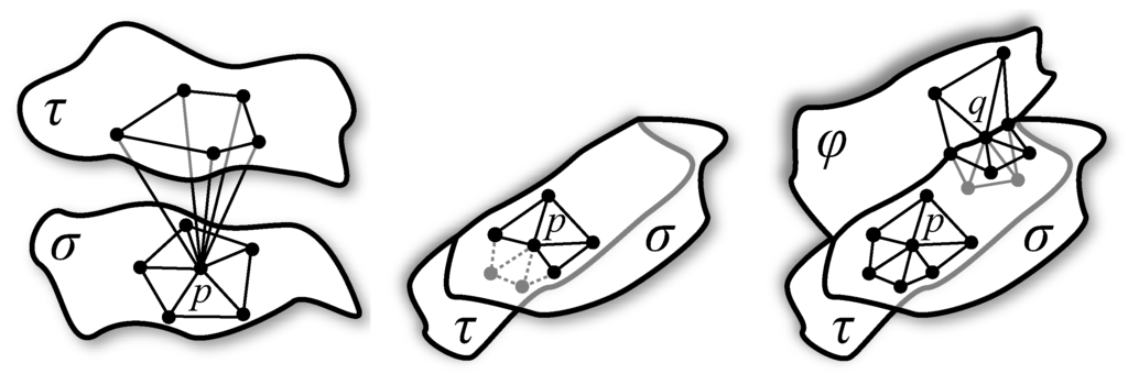
Figure 4. Disk condition: (left) Triangles incident to point $p\in \sigma$ are assumed to be restricted to σ; they do not form a disk since they form two disks pinched at p violating condition D1. (middle) The point $p\in \sigma$ has a topological disk but some of its vertices (lightly shaded) belong to τ violating condition D4. (right) Points p and q satisfy the disk condition. Point p, an interior point in σ, lies in the interior of its disk in σ. The point q, a boundary point, has three disks for each of the three 2-faces.

DelPSC $(D,\lambda )$

Protection. Let $\mathcal{B}$:= Protect($D,\lambda$). Let S be the current weighted point set. Mesh2Complex. Let $(p,\sigma )$ be any tuple where $p\in \sigma$. Let $t\in {\mathrm{Skl}}^2{S|}_{\sigma }$ be the triangle that maximizes $\mathrm{size}(t,\sigma )$ over all t and σ. Let $x\in V_t{|}_{\sigma }$ realize this maximum, say $d_1$. Let $d_2$ be the maximum radius of all vertices realized by ball, say b. (a) If condition D1 or D2 in DiskCondition(p) is violated if $d_1⩾d_2$ insert x into S else compute $\mathcal{B}:=\{\mathcal{B}\setminus b\}\cup$ RefineBall (b). (b) Else if D3 or D4 in DiskCondition(p) is violated insert x into S (c) Else if $\mathrm{size}(t,\sigma )>\lambda$ for some tuple $(t,\sigma )$ where $t\in {\mathrm{Skl}}^2{S|}_{\sigma }$ insert $x\in V_t{|}_D$ that realizes $\mathrm{size}(t,\sigma )$ into S. If S has grown in the last execution of step 2, repeat step 2. Return ${\bigcup }_i{\mathrm{Skl}}^i{S|}_D$.

Notice that in step 2(a) we refine either a ball or a triangle if either D1 or D2 is violated. However, for D3 or D4 violations in step 2(b), we only refine a triangle. This is important because D3 and D4 are not covered by Lemma 2 and may be violated no matter how small the balls are. We argue separately for D3 and D4 in the termination proof. In step 2(c) we refine triangles to reach the refinement level of the input scale.

We observe that DelPSC never inserts unweighted points inside any protecting ball. If the inserted point x in step 2(a) lies in a protecting ball $b=B(q,r)$, its weighted distance to q would be non-positive. Its weighted distance to its nearest Voronoi neighbor in S would even be smaller. Since the largest ball has a positive radius, x would not be inserted (we would call RefineBall(b) instead). If x is inserted in step 2(b), the point p is connected to a point q where either $q\notin \sigma$ or p and q are non-adjacent weighted points on a 1-face. In both cases p and q have a positive weighted distance ensured by C3.b. Therefore, a restricted triangle t incident to $pq$ has $\mathrm{size}(t,\sigma )$ positive. It follows that the point x which realizes the maximum of $\mathrm{size}(t,\sigma )$ over all t and σ has a positive weighted distance to its nearest Voronoi neighbor in S. Hence x cannot lie in a protecting ball. Finally, since $\lambda >0$, any point x inserted in step 2(c) has a positive distance to its Voronoi neighbors, and thus outside of every protecting ball. Therefore, point x has a positive weighted distance from p and hence cannot be inside a ball.

Guarantees: The analysis of the algorithm establishes two main facts: (i) the algorithm terminates, and (ii) at termination the output mesh has guarantees G1 and G2:

(G1)

For each $\sigma \in D_2$, ${\mathrm{Skl}}^2{S|}_{\sigma }$ is a 2-manifold with vertices only in σ. Further, $\mathrm{bd}\left({\mathrm{Skl}}^{2}S{|}_{\sigma }\right)$ is homeomorphic to $\mathrm{bd}\sigma$ with vertices only in $\mathrm{bd}\sigma$.

(G2)

There exists a ${\lambda }_c>0$ so that if $\lambda ⩽{\lambda }_c$, the output mesh of DelPSC(D,λ) is homeomorphic to $|D|$. Further, this homeomorphism respects stratification with vertex restrictions, that is, for $0⩽i⩽2$, ${\mathrm{Skl}}^i{S|}_{\sigma }$ is homeomorphic to $\sigma \in D_i$ where $\mathrm{bd}{\mathrm{Skl}}^{i}S{{|}_{\sigma }={\mathrm{Skl}}^{i-1}S|}_{\mathrm{bd}\sigma }$ and vertices of ${\mathrm{Skl}}^i{S|}_{\sigma }$ lie in σ.

Theorem 1 DelPSC terminates.

First, we argue that if the algorithm refines a ball, its radius is larger than a fixed positive constant. Assume that $d_1$ and $d_2$ have been defined as in the algorithm.

Consider a vertex p on a 2-face σ. The conclusion of Lemma 2 implies disk conditions D1 and D2. Therefore, if it does not hold for p, at least one of the premises of Lemma 2 does not hold. (H1) S does not satisfy the ${\lambda }_1$-property for some ${\lambda }_1>0$. (H2) Protecting balls do not satisfy C1-C3. But, when the disk condition is checked, the protecting balls satisfy condition C1, C2, C3.a, and C3.b due to Lemma 6(ii). Therefore, if H2 has failed, at least one ball has a radius more than ${\lambda }_2$ where ${\lambda }_2$ satisfies Lemma 3. The argument implies $max\{d_1,d_2\}⩾\delta =min\{{\lambda }_1,{\lambda }_2\}$. Therefore, if a ball is refined its radius is more than δ.

The entire ball refinement can be represented with trees as in the proof of Lemma 7 where a ball is refined only if its radius is at least a fixed positive constant. The argument for Lemma 7 still holds to claim that only finitely many balls are refined altogether. Therefore, the algorithm cannot refine balls forever. This also implies that the minimum size of the balls remains larger than a fixed positive constant, say $\xi >0$.

Now we argue that each point inserted by the algorithm maintains a lower bound on its distance to all other points. Then, a standard packing argument implies termination. In step 2(a), each inserted point x maintains a weighted distance at least $\delta >0$ if it is inserted because of violation of either D1 or D2. If D3 or D4 is violated in step 2(b), the weighted distance of x from p is at least half the weighted distance between p and a point q where either p and q are non-adjacent points in $D_1$ or q lies on a different 2-face. Since protecting balls have a minimum size $\xi >0$ and any two intersecting non-adjacent balls maintain a weighted distance larger than the of the radius of the smaller ball, the weighted distance between p and q is larger than a fixed positive constant. Hence, x has a distance more than a fixed positive constant from all other points. The only remaining case is step 2(c) where a point is inserted only if its weighted distance is at least $\lambda >0$ from all other points.

4. Proof of Guarantees

Let M denote the output mesh of DelPSC.

Theorem 2 M has guarantee G1.

At the end of Mesh2Complex the disk condition ensures that ${\mathrm{Skl}}^2{S|}_{\sigma }$ is a simplicial complex where each vertex v belongs to σ and has a 2-disk as its star. It follows from a result in PL topology that ${\mathrm{Skl}}^2{S|}_{\sigma }$ is a 2-manifold when DelPSC terminates.

The boundary of ${\mathrm{Skl}}^2{S|}_{\sigma }$ has all weighted vertices in $\mathrm{bd}\sigma$. Each such point p is connected to its adjacent vertices in $\mathrm{bd}\sigma$ by the disk condition. Therefore, the boundary of ${\mathrm{Skl}}^2{S|}_{\sigma }$ consists of edges that connect adjacent vertices in $\mathrm{bd}\sigma$ and hence this boundary is homeomorphic to $\mathrm{bd}\sigma$.

To prove G2 we use a result of Edelsbrunner and Shah [17] about the extended topological ball property (TBP). It can be shown that the following two properties P1 and P2 imply the extended TBP [8]. Therefore, according to the Edelsbrunner-Shah [17] result, the underlying space of ${\mathrm{Del}S|}_D$ is homeomorphic to the $|D|$ if P1 and P2 hold. Let F be a k-face of $\mathrm{Vor}S$ where S is the output vertex set.

(P1)

If F intersects an element $\sigma \in D_j\subseteq D$, the intersection is a closed $(k+j-3)$-ball.

(P2)

There is a unique lowest dimensional element ${\sigma }_F\in D$ so that F intersects ${\sigma }_F$ and only elements that are incident to ${\sigma }_F$.

Lemma 2 almost provides condition P1 except for the case that $V_p$ may intersect a patch τ where $p\notin \tau$ (Figure 7 (middle, right)). Lemma 8 establishes that this is not possible. Lemma 9 gives P2. Proofs of both of them appear in the appendix.

Lemma 8 There exists a constant ${\lambda }_c>0$ so that following holds. Let S be the point set output by DelPSC $(D,\lambda )$ for some $\lambda ⩽{\lambda }_c$. Then for each point $p\in S$, $V_p{|}_D={\bigcup }_{\sigma \ni p}{\sigma }_p$.

Lemma 9 Let S be the point set as defined in Lemma 8. Let F be a k-face in $\mathrm{Vor}S$. There is an element ${\sigma }_F\in D$ so that F intersects ${\sigma }_F$ and only elements in D that have ${\sigma }_F$ on their boundary.

Theorem 3 M satisfies G2.

For a sufficiently small $\lambda >0$, DelPSC satisfies the conditions of Lemma 8 and Lemma 9. This means that properties P1 and P2 are satisfied when λ is sufficiently small. Also when P1 and P2 are satisfied ${\bigcup }_i{\mathrm{Skl}}^{i}S{{|}_D=\mathrm{Del}S|}_D$. It follows that the Edelsbrunner-Shah conditions are satisfied for the output M of DelPSC. Thus, M has an underlying space homeomorphic to $|D|$. The homeomorphism constructed by Edelsbrunner and Shah actually respects the stratification, that is, for each $\sigma \in D_i$, ${\mathrm{Skl}}^i{S|}_{\sigma }$ is homeomorphic to σ. Also, ${\mathrm{Skl}}^1{S|}_{\sigma }$ consists of only edges that connect adjacent vertices on σ. Furthermore, property G1 holds for any output of DelPSC. This means, $\mathrm{bd}\left({\mathrm{Skl}}^{2}S{|}_{\sigma }\right)={\mathrm{Skl}}^1{S|}_{\mathrm{bd}\sigma }$. Because of the vertex balls, we also have $\mathrm{bd}\left({\mathrm{Skl}}^{1}S{|}_{\sigma }\right)={\mathrm{Skl}}^0{S|}_{\mathrm{bd}\sigma }$ trivially. Therefore, for $0⩽i⩽2$, $\mathrm{bd}\left({\mathrm{Skl}}^{i}S{|}_{\sigma }\right)={\mathrm{Skl}}^{i-1}{S|}_{\mathrm{bd}\sigma }$ and ${\mathrm{Skl}}^i{S|}_{\sigma }$ has vertices only in σ.

5. Experimental Results

The input to our software is a polygonal model which we assume approximates a PSC. A user specified threshold for dihedral angles is used to select edges of the input as sharp features (elements of $D_1$) which we protect. Non-manifold and boundary edges are also included as elements of $D_1$. In Figure 5 we show how our protection algorithm works on four different sets of curves.

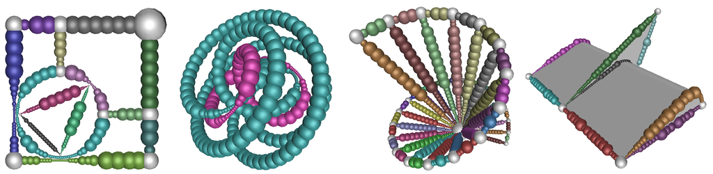
Figure 5. Protection: (left) A 2d example of curve protection. (middle) 2 different 3d examples of curve complexes where we have run Protect. (right) The final set of protecting balls returned by Mesh2Complex on the Wedge model.

In Table 1 we show both the time to protect curves as well as the time to generate the surface mesh for twelve different datasets. All experiments were run on a PC with a 2.8 GHz CPU and 2 GB RAM. We set the parameter λ to 5% of the minimum dimension of the bounding box for each model. Those datasets which took no time for protection had no sharp features in their input; the PSC they approximate was assumed to be a single smooth patch. The majority of the datasets were meshed in under one minute, only those with complicated topologies took longer.

Table 1. Protection and Meshing times for our datasets.

Dataset	Protection Time	Meshing Time	# of vertices
9 Holes	0.0 s	105.6 s	8725
Arm	52.6 s	339.7 s	20692
Cog	1.4 s	56.2 s	7697
Guide	2.6 s	22.9 s	4414
Horn	0.0 s	21.5 s	3192
Lock	10.6 s	26.6 s	5314
Octo	0.0 s	7.3 s	1410
Part	0.2 s	23.2 s	4261
Plate	17.9 s	83.9 s	9773
Pump	19.1 s	319.6 s	20301
Swirl	0.0 s	61.1 s	6880
Wedge	0.2 s	13.2 s	3080

Table 1. Protection and Meshing times for our datasets.

Dataset	Protection Time	Meshing Time	# of vertices
9 Holes	0.0 s	105.6 s	8725
Arm	52.6 s	339.7 s	20692
Cog	1.4 s	56.2 s	7697
Guide	2.6 s	22.9 s	4414
Horn	0.0 s	21.5 s	3192
Lock	10.6 s	26.6 s	5314
Octo	0.0 s	7.3 s	1410
Part	0.2 s	23.2 s	4261
Plate	17.9 s	83.9 s	9773
Pump	19.1 s	319.6 s	20301
Swirl	0.0 s	61.1 s	6880
Wedge	0.2 s	13.2 s	3080

In Figure 6 we show output meshes for various input shapes. These meshes include four smooth shapes (9 Holes, Horn, Octo, and Swirl), two non-manifolds (Horn and Wedge), and eight piecewise-smooth shapes (Part, Guide, Wedge, Cog, Arm, Lock, Pump, and Plate). DelPSC has been used to mesh dozens of other models; further experimentation was presented in a recent multimedia presentation [16].

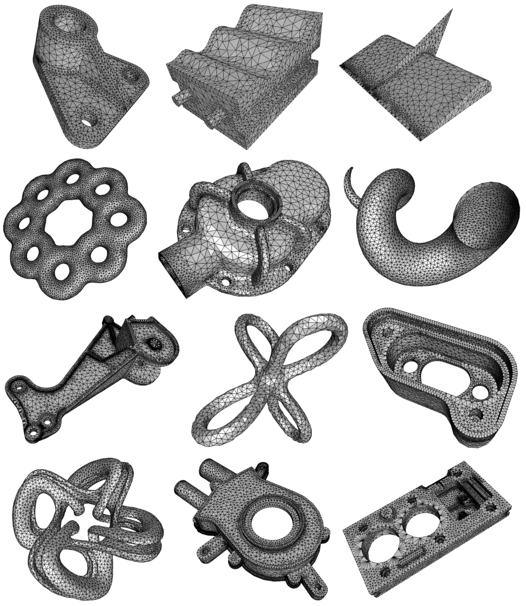
Figure 6. DelPSC output meshes. Left to right, top to bottom: Part, Guide, Wedge, 9 Holes, Cog, Horn, Arm, Octo, Lock, Swirl, Pump, and Plate, models.

6. Conclusions

We have presented a new practical algorithm to mesh a wide variety of geometric domains with the Delaunay refinement technique. Unlike previous approaches, this algorithm computes the protecting balls on the fly and thus gets rid of expensive computations to fix them a priori. The only domain dependent numerical computations are: (i) computing intersection points of the input curves with spheres (to determine the end points of ${\mathrm{seg}}_{\sigma }\left(b\right)$) and (ii) computing intersection of Voronoi edges with surface patches (to determine restricted triangles and their sizes; these computations are always necessary for the restricted Delaunay mesh [3, 8]). These computations are much easier than normal variation and gap size computations as proposed in [8].

The output mesh maintains a manifold property and with increasing level of refinement captures the topology of the input. In practice, most of the time this level is achieved fast with only the disk condition. An interesting aspect of the algorithm is that the input ‘non-smooth features’ are preserved in the output. However, one requirement is that an explicit representation of these features must be available so that we can sample them as a bootstrap step. For polygonal inputs, it is relatively easy to partition the space into a PSC using the thresholding approach described for the experiments, but for implicitly represented PSCs this may be more challenging.

Our experimental results, implemented in CGAL [18], further validate our claims of practicality and implementability. Some additional implementation details were reported a recent video presentation [16]. We note that this implementation of the algorithm uses a variation on the disk condition. Condition D3 has been changed to only require that each point p sampled from a curve $\sigma \in D_1$ is not connected to any non-adjacent points on σ (as opposed to requiring global disconnection from all non-adjacent samples in $D_1$).

In applications, sometimes it is desired that the mesh elements have good aspect ratios and their size adapts to the input feature size. Our algorithm can be easily extended to guarantee bounded aspect ratio for most triangles except for the ones near non-smooth regions. However, it cannot produce meshes with true adaptive sizing. Insertions to satisfy the disk condition can cause some varied sizing in the output meshes creating a non-uniform appearance. Many of our output meshes exhibit this property; it is caused by λ (which controls only the maximum triangle size) having a value larger than the triangle size needed to fulfill the disk condition. We note that since adaptive meshing ultimately requires an estimate of the input feature size, it may not be possible to produce such meshes without expensive computations. We also note that it should be possible to extend our algorithm to volumes using an approach similar to [19].

7. Proofs of lemmas in Section 2

For proving Lemma 2 we need some standard results from sampling theory [20, 21]. Recall that we have assumed each 2-face in the domain to be a compact subset of a smooth ($C^2$) 2-manifold without boundary. This helps us to carry forward a result on normal variation from smooth surfaces straightforwardly to the surface patches with boundaries. If surface elements are not assumed to be a subset of smooth surfaces without boundary, normal variation proof becomes more complicated with a worse error bound.

Let σ be any 2-face which by assumption is a subset of a smooth 2-manifold ${\sigma }^{*}$ without boundary. The surface normal ${\mathbf{n}}_x$ to σ at x is the surface normal of ${\sigma }^{*}$ at x. Let M denote the medial axis of ${\sigma }^{*}$, that is, M is the closure of all points in ${\mathbb{R}}^3$ which have two or more closest points in ${\sigma }^{*}$. Borrowing from [20], we define the local feature size ${\mathrm{lfs}}_x=d(x,M)$. In the analysis, we use a global lower bound on the $\mathrm{lfs}$ function. We define:

$${\rho }_{\sigma }=\underset{x\in \sigma }{inf}{\mathrm{lfs}}_x.$$

Recall that $\widehat{d}(x,y)$ denotes the weighted distance between two weighted points x and y, that is, $\widehat{d}(x,y)=\sqrt{d{(x,y)}^2-{\omega }_x^2-{\omega }_y^2}$ where ${\omega }_x$ and ${\omega }_y$ are the weights of x and y respectively. For a triangle t, consider the disk whose weighted distance to all of t’s vertices (possibly weighted) is zero. The radius of this disk is called the orthoradius of t.

Lemma 10 Let $\epsilon \in (0,1/3)$ be some constant.

(i)

For any two points x and y in σ such that $d(x,y)⩽\epsilon {\rho }_{\sigma }$,

(a)

the angle between the surface normals ${\mathbf{n}}_x$ at x and ${\mathbf{n}}_y$ at y is at most $2\epsilon$;

(b)

the angle between $xy$ and the surface normal at x is at least $arccos(\epsilon /2)$.

(ii)

Let $pqr$ be a triangle with vertices on σ which are possibly weighted with a weight $\omega {\rho }_{\sigma }$ for $\omega <1$. Furthermore, let the orthoradius of $pqr$ be no more than $\epsilon {\rho }_{\sigma }$. Then, ${\angle }_a({\mathbf{n}}_{pqr},{\mathbf{n}}_p)⩽5\sqrt{{\epsilon }^2+{\omega }^2}$.

(i.a) Follows from the normal variation result in [22].

(i.b) Follows from the Edge Normal Lemma in [21].

(ii) Let R and $\widehat{R}$ be the circumradius and orthoradius of $pqr$ respectively. For a sufficiently small ω, the circumcenter x lies inside the orthocircle of $pqr$. Then, minimum weighted distance of x to any of three vertices of $pqr$, is a lower bound on $\widehat{R}$, that is,

$$\begin{array}{ccc}\hfill R^2-{\omega }^2{\rho }_{\sigma }^2& ⩽& {\widehat{R}}^2\hfill \\ \hfill R^2& ⩽& {\epsilon }^2{\rho }_{\sigma }^2+{\omega }^2{\rho }_{\sigma }^2\hfill \\ & ⩽& ({\epsilon }^2+{\omega }^2){\rho }_{\sigma }^2.\hfill \end{array}$$

Without loss of generality, assume that p subtends the largest angle in $pqr$. Plugging $R_{pqr}=R⩽\sqrt{{\epsilon }^2+{\omega }^2}{\rho }_{\sigma }$ and using ${\mathrm{lfs}}_{(}p)⩾{\rho }_{\sigma }$ in the Triangle Normal Lemma (Lemma 3.5 in [21]), we get that

$$\begin{array}{ccc}\hfill {\angle }_a({\mathbf{n}}_p,{\mathbf{n}}_{pqr})& ⩽& arcsin\sqrt{{\epsilon }^2+{\omega }^2}+arcsin\left(\frac{2}{\sqrt{3}}\left(2arcsin\sqrt{{\epsilon }^2+{\omega }^2}\right)\right)\hfill \\ & ⩽& 5\sqrt{{\epsilon }^2+{\omega }^2}.\hfill \end{array}$$

Consider a weighted vertex $p\in S$ on a 2-face σ. For any facet F of $V_p$, we use $H_F$ to denote the plane of F. Let $\lambda ⩽\frac{1}{32}{\rho }_{\sigma }$. Let $B=B(p,2\lambda )$. By the Feature Ball Lemma in [21] $B\cap \sigma$ is a 2-disk.

Lemma 11 For any facet F of $V_p$, if $H_F$ intersects $B\cap \sigma$, then $\angle ({\mathbf{n}}_p,H_F)⩽arcsin(1/16)$ and both $H_F\cap B\cap \sigma$ and $F\cap B\cap \sigma$ contain no closed curve.

Let $pq$ be the dual Delaunay edge of F where $H_F$ intersects $pq$ at x. We have $\widehat{d}(p,x)=\widehat{d}(q,x)⩽\sqrt{4{\lambda }^2-w_p^2}$ from which we can derive that $d(q,x)⩽\sqrt{4{\lambda }^2-w_p^2+w_q^2}⩽\sqrt{5}\lambda$. It follows that

$$d(p,q)⩽d(p,x)+d(q,x)⩽(2+\sqrt{5})\lambda ⩽5\lambda .$$

which is less than $\frac{1}{8}{\rho }_{\sigma }$. By Lemma 10(ib), $\angle ({\mathbf{n}}_p,H_F)=\pi /2-\angle ({\mathbf{n}}_p,pq)⩽arcsin(1/16)$. There is no closed curve in $H_F\cap B\cap \sigma$ because such a closed curve would bound a 2-disk in $B\cap \sigma$, which would contain a point x such that $\angle ({\mathbf{n}}_x,H_F)=\pi /2$. This is a contradiction because $\angle ({\mathbf{n}}_x,H_F)⩽\angle ({\mathbf{n}}_x,{\mathbf{n}}_p)+\angle ({\mathbf{n}}_p,H_F)⩽1/8+arcsin(1/16)<\pi /2$ by Lemma 10(i.a). Since $H_F\cap B\cap \sigma$ contains no closed curve, neither does $F\cap B\cap \sigma$. This proves the claim.

Lemma 12 For any facet F of $V_p$, if $d(p,F)⩽\lambda$ and conditions C1-C3 hold, then $F\cap B\cap \sigma$ is either empty or a single open curve.

We assume that $H_F$ intersects $B\cap \sigma$ since otherwise $F\cap B\cap \sigma$ is empty and there is nothing to prove. First, we show that if $H_F$ is within a distance of λ from p, $H_F\cap B\cap \sigma$ is a single open curve. Consider the disk $H_F\cap B$. Let $\overrightarrow{d}$ be the projection of ${\mathbf{n}}_p$ onto $H_F$. Let $L\subset H_F$ be the line through the center of $H_F\cap B$ orthogonal to $\overrightarrow{d}$. Let x be any point in $H_F\cap B\cap \sigma$. The angle between $px$ and the tangent plane at p is at most $arcsin(1/32)$ by Lemma 10(i.b). We already proved that $\angle ({\mathbf{n}}_p,H_F)⩽arcsin(1/16)$. We are interested in an upper bound on the distance $d(x,L)$. Let $x^{*}$ be the orthogonal projection of x onto L. Consider the triangle $px{x}^{*}$. Observe that $\angle xp{x}^{*}$ is the angle between $px$ and the tangent plane at p and $\angle p{x}^{*}x$ is at least $\pi /2-\angle ({\mathbf{n}}_p,H_F)$. We obtain

$$d(x,x^{*})⩽d(p,x)\frac{sinarcsin(1/32)}{cosarcsin(1/16)}⩽(0.035)\left(2\lambda \right)⩽0.07\lambda .$$

Let $L^{*}\subset H_F$ be the strip of points at distance $0.07\lambda$ or less from L. Since the radius of B is $2\lambda$ and $H_F$ is at most λ distance from p, the radius of $H_F\cap B$ is at least $\sqrt{3}\lambda$. It follows that the boundary of $H_F\cap B$ intersects $L^{*}$ in two disjoint circular arcs, say A and $A^{\prime }$.

We already proved that there is no closed curve in $H_F\cap B\cap \sigma$ (Lemma 11). Now we show that $H_F\cap B\cap \sigma$ cannot contain two open curves. First, we eliminate the case where $H_F\cap B\cap \sigma$ are two open curves each having an end point on $\mathrm{bd}\sigma$. For this to happen, F has to intersect $\mathrm{bd}\sigma$ in more than one point, which is impossible by Lemma 1 if the protecting balls satisfy condition C1-C3. Therefore, we can assume that if $H_F\cap B\cap \sigma$ has two open curves, at least one, say C, has both end points on the circular arcs A and/or $A^{\prime }$. Consider the case where C has end points both in A and $A^{\prime }$. The other curve, say $C^{\prime }$, in $H_F\cap B\cap \sigma$ must have an end point in at least one of A and $A^{\prime }$. It follows that either A or $A^{\prime }$ should have an end point of both C and $C^{\prime }$. Without loss of generality, assume that A has end points of both C and $C^{\prime }$ and let s and t be these end points. We observe that the line segment $st$ cannot make an angle with L less than the least angle made between L and a tangent to A. This least angle is made by the tangent to A at any of its end points. Since the width of $L^{*}$ is $0.07\lambda$ and the radius of $H_F\cap B$ is at least $\sqrt{3}\lambda$, this least angle is more than $\frac{\pi }{2}-arcsin(0.035/\sqrt{3})$. Therefore, $st$ makes an angle of at least $\frac{\pi }{2}-arcsin(0.035/\sqrt{3})$ with L, or equivalently of at most $arcsin(0.035/\sqrt{3})<0.03$ with $\overrightarrow{d}$. Since $\angle \overrightarrow{d},{\mathbf{n}}_s⩽\angle \overrightarrow{d},{\mathbf{n}}_p+\angle {\mathbf{n}}_p,{\mathbf{n}}_s⩽arcsin(1/16)+(1/8)⩽0.2$, $st$ makes an angle of at most $0.23$ radians with ${\mathbf{n}}_s$. The line of $st$ intersects σ at two points, namely at s and t, where $\angle st,{\mathbf{n}}_s⩽0.23$. Here we can use the Long Distance Lemma in [21] to obtain $d(s,t)⩾2{\rho }_{\sigma }cos0.23⩾62\lambda$ which contradicts $d(s,t)⩽2\times 0.07\lambda =0.14\lambda$.

Next, consider the case where C has both endpoints on a single arc, say A. Taking these end points as s and t we can argue as in the previous paragraph to reach a contradiction.

Third, we claim that for any facet F of $V_p$, if F intersects $B\cap \sigma$, $F\cap B\cap \sigma$ is a single open curve with endpoints in $\mathrm{bd}F$ or in $\mathrm{bd}\sigma$. We already proved that there is no closed curve in $F\cap B\cap \sigma$. Since F does not have any tangential contact with σ, $F\cap B\cap \sigma$ is a set of open curves and the endpoints of any open curve in $F\cap \sigma$ thus lie in $\mathrm{bd}F$ or in $\mathrm{bd}\sigma$. Assume to the contrary that $F\cap B\cap \sigma$ contains two open curves, say ξ and ${\xi }^{\prime }$. By our assumption, $H_F$ is within a distance of λ from p. We have shown before that $H_F\cap B\cap \sigma$ is a single open curve. Follow $H_F\cap B\cap \sigma$ from ξ to ${\xi }^{\prime }$. When we leave ξ, we must leave F at a Voronoi edge $e\subset \mathrm{bd}F$. Afterwards, we stay in the plane $H_F$ and we must cross the support line of e again in order to reach ${\xi }^{\prime }$. Therefore, some tangent to $H_F\cap B\cap \sigma$ is parallel to e. However, the angle between the surface normal at some point on $H_F\cap B\cap \sigma$ and ${\mathbf{n}}_p$ would then be at least $\pi /2-\angle {\mathbf{n}}_p,e⩾\pi /2-5\sqrt{2{(\lambda /{\rho }_{\sigma })}^2}$ by Lemma 10(ii) since $\epsilon ,\omega ⩽\lambda /{\rho }_{\sigma }$. This contradicts Lemma 10(i.a) proving the claim.

Recall that ${\sigma }_p$ denote the components of $V_p{|}_{\sigma }$ that intersect a Voronoi edge of $V_p$. We show that ${\sigma }_p$ intersect $V_p$ and its faces in topological balls if S has the λ-size property for a sufficiently small λ. We need the following result which says that when λ is sufficiently small, each Voronoi cell $V_p$ contains at least one Voronoi edge intersecting σ if $p\in \sigma \in D_2$.

Lemma 13 There exists a $\lambda >0$ so that if S satisfies the λ-size property, then ${\sigma }_p$ is non-empty for any $p\in \sigma$

Suppose that ${\sigma }_p$ is empty, that is, no Voronoi edge of $V_p$ intersects σ. By our assumption $\mathrm{bd}\sigma$ is non-empty and let $q\in \sigma$ be a weighted point in $\mathrm{bd}\sigma$. Because of Lemma 1, an edge of $V_q$ has to intersect σ. Consider walking on a path in σ from p to q. Let $p=p_0,p_1,..,p_k=q$ be sequence of vertices whose Voronoi cells are encountered along this walk. Since no edge of $V_p$ intersects σ and some edge of $V_q$ intersects σ, there exists two consecutive vertices $p_i$ and $p_{i+1}$ in this sequence so that no edge of $V_{p_i}$ intersects σ whereas some edge of $V_{p_{i+1}}$ does intersect σ. By Lemma 2 we can claim that ${\sigma }_{p_{i+1}}$ is a disk. A boundary cycle of ${\sigma }_{p_i}$ overlaps with the boundary of ${\sigma }_{p_{i+1}}$. This is impossible as the curves on the boundary of ${\sigma }_{p_{i+1}}$ intersect Voronoi edges whereas those on the boundary of ${\sigma }_{p_i}$ do not.

Now we are ready to prove the main claim of Lemma 2. Figure 7 explains more about its implications.

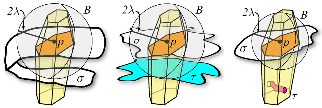
Figure 7. (left) A 2-face σ has intersected $V_p$ where ${\sigma }_p$ is not topological disk, this is not possible by R1. (middle) ${\sigma }_p$ is a disk but another face τ where $p\notin \tau$ intersects some edge of $V_p$. It does not violate R1 but violates Lemma 8. (right) Within B, σ intersects $V_p$ in a topological disk. There is a different component (τ) which does not intersect any Voronoi edge and hence does not contribute any dual restricted triangle incident to p. R1 does not prevent it though Lemma 8 does.

Lemma 14 There is a $\lambda >0$ so that if H1 and H2 of Lemma 2 are satisfied, then ${\sigma }_p$ is a topological disk. Furthermore, each Voronoi edge and facet that intersects ${\sigma }_p$ does so in a single point and single open curve respectively.

Recall $B=B(p,2\lambda )$. Consider an edge of $V_p$ that intersects $B\cap \sigma$. By Lemma 10(ii), $\angle {\mathbf{n}}_p,e⩽5\sqrt{2{(\lambda /{\rho }_{\sigma })}^2}$. Then, by Lemma 10(i.a), $B\cap \sigma$ is monotonic in the direction of e when λ is sufficiently small. Therefore, e intersects $B\cap \sigma$ and hence ${\sigma }_p$ at most once. Each facet of $V_p$ that intersects $B\cap \sigma$ intersects it in a single open curve by Lemma 12. This completes the proof of the second part of the lemma.

We show that the argument of Lemma 4.12 in [4] can be used here to establish that ${\sigma }_p$ is a topological disk. Following the notation in the proof of this lemma, let us call a cycle in ${\sigma }_p$ that intersects a Voronoi edge a type 1 cycle. Let X denote the set of type 1 cycles. Each Voronoi facet containing a point in X has a Voronoi edge intersecting ${\sigma }_p$. By H1, this intersection point is within λ distance of p. Therefore, B intersects all Voronoi facets that contain a point in X. These Voronoi facets intersect $B\cap \sigma$ in a single open curve which is in B. Also, if $V_p$ intersects $\mathrm{bd}\sigma$, the entire curve segment $V_p\cap \mathrm{bd}\sigma$ is contained in the protecting ball of p. This means each point of X is within λ distance of p. Since each cycle in X is a piecewise smooth closed curve where each piece is either an open curve contained in a Voronoi facet or a segment of $V_p\cap \mathrm{bd}\sigma$, it is contained completely in B. Therefore, each boundary of ${\sigma }_p$ which intersects a Voronoi edge lies in B.

Consider the arrangement of closed curves in X on $B\cap \sigma$ which is a topological disk according to the Feature Ball Lemma [21]. Let $C\in X$ be a closed curve which does not contain any other curve of X inside. At least one such curve exists since X is not empty by Lemma 13. The closed curve C must bound a disk, say D in σ. At this point we can invoke the proof of Lemma 4.12 in [4] to prove that $D={\sigma }_p$ establishing our first claim. The boundary $\mathrm{bd}{\sigma }_p$ lies in X which has at most a single interval in any Voronoi facet as we argued above. This establishes our second claim.

[Proof of Lemma 2.]

Proof of R1: Follows from Lemma 14.

Proof of R2: Since conditions C1-C3 hold, Lemma 1 can be applied. The conclusion of this lemma implies R2.

[Proof of Lemma 4.] Cover affects only the sequence of balls $b_0,b_1,...,b_k$ as referred in its description. By construction the new balls cover entire curve segment $\sigma (x,y)$ and vertex balls are not changed. So, C1 and the first part of C2 are satisfied. To prove the second part consider a ball $b_i=B(c_i,r_i)$. We have following cases:

Case 1 ($i=0$): We need to examine the effect of the new ball $b_1$ onto $b_0$. First notice that ${\mathrm{seg}}_{\sigma }\left(b_0\right)$ cannot contain $c_1$ by construction. Therefore, C3.a holds trivially. If $b_1$ is not created with the end game, the radius of $b_1$ is α and $d(c_0,c_1)<r_0+\alpha /3<r_0+r_1/3$ where $r_1=\alpha <r_0$ by construction. This satisfies C2. If $b_1$ is created with the end game, then two cases occur. If $b_1$ is the enlarged aiding ball ${\beta }_1$, its radius is $2\alpha /3$. Then, $d(c_0,c_1)=r_0<r_0+r_1/3$. This satisfies C2. In the case where $b_1$ is not the enlarged aiding ball, its radius is $\frac{7}{6}\alpha$. We can similarly argue that $d(c_0,c_1)<r_0+\alpha /3=r_0+\frac{2}{7}{r}_1$. So, $b_0$ satisfies C2.

Case 2 ($i=k$): In this case the center $c_{k-1}$ of $b_{k-1}$ cannot lie in ${\mathrm{seg}}_{\sigma }\left(b_k\right)$ by construction. So, C3.a holds trivially. The ball $b_{k-1}$ is necessarily created with the end game. If $b_{k-1}$ is enlarged ${\beta }_{k-1}$, $d(c_{k-1},c_k)<r_k+\alpha /3=r_k+r_{k-1}/2$ satisfying C2. In the case where $b_{k-1}$ is not the enlarged aiding ball, its radius is $\frac{7}{6}\alpha$. Then, $d(c_k,c_{k-1})<r_k+\alpha =r_k+\frac{6}{7}{r}_{k-1}$ satisfying C2.

Case 3 ($i\ne 0andi\ne k$): If $b_i$ is adjacent to $b_0$ and $b_k$, it satisfies C2 by arguments in previous two cases. Also, $b_i$ is not large enough to contain $c_0$ or $c_k$. Hence C3.a also holds. Now consider the case where $b_i$ is adjacent to another ball b where $b\ne b_0$ and $b\ne b_k$. If neither $b_i$ nor b is created by end game, we have $d(c,c_i)⩽r_i+\alpha /3=r_i+r_i/3$ satisfying C2. Also, in this case $d_{\sigma }(c,c_i)⩾\frac{4}{3}\alpha =\frac{4}{3}{r}_i$ which satisfies C3.a. We are left with the case when either of b and $b_i$ is created with the end game. With similar arguments, one can check that C2 and C3.a hold in these cases too.

8. Proofs of lemmas in Section 4

[Proof of Lemma 8.] Recall that ${\sigma }_p$ denotes the set of connected components in $V_p{|}_{\sigma }$ intersecting a Voronoi edge. We are required to prove that $V_p{|}_D={\bigcup }_{\sigma \ni p}{\sigma }_p$. Assume to the contrary that $\bigcup {\sigma }_p\subset V_p{|}_D$. Let C be any connected component in $V_p{|}_D\setminus \bigcup {\sigma }_p$. and $C\subset {\sigma }^{\prime }$ where ${\sigma }^{\prime }\ne \sigma$. Voronoi cells partition ${\sigma }^{\prime }$. A path on ${\sigma }^{\prime }$ from $\mathrm{bd}C$ to a sample point $q\in {\sigma }^{\prime }$ passes through the connected components of this partition. We must encounter two adjacent components along this path, say $C^{\prime }$ and $C^{\prime \prime }$, where $C^{\prime }={\sigma }_s^{\prime }$ for $s\notin {\sigma }^{\prime }$ and $C^{\prime \prime }={\sigma }_r^{\prime }$ for some $r\in {\sigma }^{\prime }$. This holds because the first and last components satisfy this property. Then, by PSC Lemma (Lemma 2), $C^{\prime \prime }={\sigma }_r^{\prime }$ is a topological disk intersecting Voronoi edges of $V_r$. Since $C^{\prime }$ and $C^{\prime \prime }$ are adjacent, there is a Voronoi edge e incident to both $V_r$ and $V_s$ which is intersected by ${\sigma }_r^{\prime }$. This means ${\mathrm{Umb}}_r$ has a triangle with a vertex s which is not in ${\sigma }^{\prime }$, a condition forbidden by DiskCondition. Since we are considering the point set output by DelPSC, the DiskCondition must have been satisfied.

[Proof of Lemma 9.] Case 1: F is a Voronoi cell $V_p$. Let ${\sigma }_F\in D$ be the lowest dimensional element containing p. We claim all elements in D intersecting F have ${\sigma }_F$ in their boundaries and thus ${\sigma }_F$ is unique. If not, let there be another ${\sigma }^{\prime }\in D$ where ${\sigma }_F\neg \subset \mathrm{bd}{\sigma }^{\prime }$. Notice that $p\notin {\sigma }_F\cap {\sigma }^{\prime }$ since otherwise ${\sigma }_F\cap {\sigma }^{\prime }$ is either an element of D whose dimension is lower than ${\sigma }_F$ or ${\sigma }_F\cap {\sigma }^{\prime }={\sigma }_F$ both of which are impossible. It follows that $p\notin {\sigma }^{\prime }$. But we already argued above that $V_p$ intersects only elements in D that contain p.

Case 2: F is a Voronoi facet $V_{pq}$. Let ${\sigma }_F$ be a lowest dimensional element that F intersects. Assume there is another ${\sigma }^{\prime }$ intersecting F where ${\sigma }_F\neg \subset \mathrm{bd}{\sigma }^{\prime }$. We go over different dimensions of ${\sigma }^{\prime }$ each time reaching a contradiction.

Assume ${\sigma }^{\prime }\in D_{⩽2}$; ${\sigma }^{\prime }$ intersects F and does not contain ${\sigma }_F$ on its boundary. Two cases can arise. Either (i) ${\sigma }_F$ and ${\sigma }^{\prime }$ are disjoint within $V_p$ or $V_q$, or (ii) ${\sigma }_F$ and ${\sigma }^{\prime }$ have a common boundary in $V_p$ and $V_q$. Case (i) cannot happen due to the claim in Case 1. For (ii) to happen, both p and q have to be on the common boundaries of ${\sigma }_F$ and ${\sigma }^{\prime }$, which means that p and q have to be on some element in $D_{⩽1}$. Observe that p and q are non-adjacent since otherwise $V_{pq}$ has to intersect the common boundary of ${\sigma }_F$ and ${\sigma }^{\prime }$ whose dimension is lower than that of ${\sigma }_F$. But this would contradict the disk condition that no two non-adjacent vertices in $D_1$ are connected by a restricted edge.

The above argument implies that all elements intersecting F have ${\sigma }_F$ as a subset.

Case 3: F is a Voronoi edge. Certainly F cannot intersect a 2-face ${\sigma }_F$ more than once due to Lemma 2 (R1). The other possibility is that $F=V_t$, $t\in {\mathrm{Skl}}^2{S|}_{{\sigma }_F}$, and F intersects ${\sigma }^{\prime }\ne {\sigma }_F$. But then a Voronoi cell adjacent to F would intersect two 2-faces ${\sigma }_F$ and ${\sigma }^{\prime }$ and t is in both ${\mathrm{Skl}}^2{S|}_{{\sigma }_F}$ and ${\mathrm{Skl}}^2{S|}_{{\sigma }^{\prime }}$ violating the disk condition.

References

- Chew, L.P. Guaranteed-quality triangular meshes. Technical Report TR-89-983, Comp. Science Department, Cornell University: Ithaca, NY, USA, 1989. [Google Scholar]
- Chew, L.P. Guaranteed-quality mesh generation for curved surfaces. In Proceedings of the 9th Symposium on Computational Geometry, San Diego, CA, USA, May 19-21, 1993; pp. 274–280.
- Boissonnat, J.D.; Oudot, S. Provably good sampling and meshing of surfaces. Graph. Models 2005, 67, 405–451. [Google Scholar] [CrossRef]
- Cheng, S.W.; Dey, T.K.; Ramos, E.A.; Ray, T. Sampling and meshing a surface with guaranteed topology and geometry. SIAM J. Comput. 2007, 37, 1199–1227. [Google Scholar] [CrossRef]
- Shewchuk, J.R. Mesh generation for domains with small angles. In Proceedings of the 16th Symposium on Computational Geometry, Hong Kong, China, June 12-14, 2000; pp. 1–10.
- Boissonnat, J.D.; Oudot, S. Provably good sampling and meshing of Lipschitz surfaces. In Proceedings of the 22nd Symposium on Computational geometry, Sedona, AZ, USA, June 5-7, 2006; pp. 337–346.
- Rineau, L.; Yvinec, M. Meshing 3D Domains Bounded by Piecewise Smooth Surfaces. In Proceedings of the 16th International Meshing Roundtable, Seattle, WA, USA, October 14-17, 2007; pp. 443–460.
- Cheng, S.W.; Dey, T.K.; Ramos, E.A. Delaunay refinement for piecewise smooth complexes. In Proceedings of the 18th ACM-SIAM Symposium on Discrete Algorithms, New Orleans, LA, USA, January 7-9, 2007; pp. 1096–1105.
- Cheng, S.W.; Poon, S.H. Three-Dimensional Delaunay Mesh Generation. Disc. Comput. Geom. 2006, 36, 419–456. [Google Scholar] [CrossRef]
- Cohen-Steiner, D.; de Verdière, É.C.; Yvinec, M. Conforming Delaunay triangulations in 3D. Comput. Geom. 2004, 28, 217–233. [Google Scholar] [CrossRef]
- Murphy, M.; Mount, D.M.; Gable, C.W. A Point-Placement Strategy for Conforming Delaunay Tetrahedralization. Int. J. Comput. Geom. Appl. 2001, 11, 669–682. [Google Scholar] [CrossRef]
- Aurenhammer, F. Power Diagrams: Properties, Algorithms and Applications. SIAM J. Comput. 1987, 16, 78–96. [Google Scholar] [CrossRef]
- Edelsbrunner, H. Geometry and Topology for Mesh Generation; Cambridge University: Cambridge, UK, 2001. [Google Scholar]
- Ruppert, J. A Delaunay Refinement Algorithm for Quality 2-Dimensional Mesh Generation. J. Algorithms 1995, 18, 548–585. [Google Scholar] [CrossRef]
- Cheng, S.W.; Dey, T.K.; Levine, J.A. A practical Delaunay meshing algorithm for a large class of domains. In Proceedings of the 16th International Meshing Roundtable, Seattle, Washington, USA, October 14-17, 2007; pp. 477–494.
- Dey, T.K.; Levine, J.A. DelPSC: a Delaunay mesher for piecewise smooth complexes (multimedia submission). In Proceedings of the 24th ACM Symposium on Computational Geometry, College Park, MD, USA, June 9-11, 2008; pp. 220–221.
- Edelsbrunner, H.; Shah, N.R. Triangulating Topological Spaces. Int. J. Comput. Geometry Appl. 1997, 7, 365–378. [Google Scholar] [CrossRef]
- Cgal. Computational Geometry Algorithms Library. Available online: http://www.cgal.org (accessed September 25, 2009).
- Oudot, S.; Rineau, L.; Yvinec, M. Meshing volumes bounded by smooth surfaces. In Proceedings of the 14th International Meshing Roundtable, San Diego, CA, USA, September 11-14, 2005; pp. 203–219.
- Amenta, N.; Bern, M. Surface reconstruction by Voronoi filtering. Disc. Comput. Geom. 1999, 22, 481–504. [Google Scholar] [CrossRef]
- Dey, T.K. Curve and Surface Reconstruction: Algorithms with Mathematical Analysis; Cambridge University: New York, NY, USA, 2007. [Google Scholar]
- Amenta, N.; Dey, T. Normal variation with adaptive feature size. Available online: http://www.cse.ohio-state.edu/ tamaldey/paper/norvar/norvar.pdf (accessed September 25, 2009).
© 2009 by the authors; licensee Molecular Diversity Preservation International, Basel, Switzerland. This article is an open access article distributed under the terms and conditions of the Creative Commons Attribution license http://creativecommons.org/licenses/by/3.0/.