Article

A Prior-Guided Structure-Aware Multi-Objective Differential Evolution Method for High-Dimensional Feature Selection

1
School of Intelligent Medicine and Information Engineering, Jiangxi University of Chinese Medicine, Nanchang 330004, China
2
School of Mathematics and Information Science, Nanchang Normal University, Nanchang 330032, China
*
Author to whom correspondence should be addressed.
Algorithms 2026, 19(9), 797; https://doi.org/10.3390/a19090797
Submission received: 5 August 2026 / Revised: 14 September 2026 / Accepted: 15 September 2026 / Published: 17 September 2026
(This article belongs to the Special Issue Algorithms for Feature Selection and Feature Reduction)

Abstract

Multi-objective feature selection provides an effective framework for high-dimensional data analysis by jointly considering classification performance and feature subset size. However, redundant and irrelevant features may degrade the quality of the initial search distribution, and population aggregation may reduce the structural diversity of non-dominated feature subsets. To address these issues, this paper proposes PGS-MODE-FS, a prior-guided and structure-aware multi-objective differential evolution method for high-dimensional feature selection. Specifically, feature–class relevance and feature redundancy are integrated into a unified feature importance measure to guide the generation of candidate solutions with different sparsity levels. The same feature-priority information is further used to construct a Top-k activated subspace, in which individuals are assigned to multiple islands according to their structural differences on informative features, thereby promoting diverse evolutionary search. Experiments on 17 public and biomedical datasets, including parameter analysis, comparative experiments, and ablation studies, demonstrate that PGS-MODE-FS achieves competitive performance in solution-set quality, classification accuracy, feature reduction, and computational efficiency. Further diversity analysis shows that the proposed multi-island mechanism effectively preserves structural diversity during evolution.

1. Introduction

High-dimensional data usually contain a large number of redundant, irrelevant, or even noisy features, while limited sample sizes and complex feature relationships further increase the difficulty of identifying informative features. This not only increases the computational burden of model training and search, but also tends to cause overfitting and reduce the stability of classification results [1,2]. Feature selection provides an important dimensionality reduction strategy for high-dimensional classification by selecting variables with stronger discriminative ability from the original feature set. Compared with feature extraction methods, it can also better preserve the semantic meaning and interpretability of the original features [3,4].
Feature selection is not merely a problem of maximizing classification accuracy. Existing studies have shown that classification error and the number of selected features are two typical and mutually conflicting optimization objectives in feature selection [5]. In application scenarios such as pattern recognition, bioinformatics, medical data analysis, and text classification, researchers usually aim to achieve satisfactory classification performance while selecting as few features as possible, thereby reducing model complexity and practical application costs [6]. Therefore, modeling feature selection as a multi-objective optimization problem better aligns with practical requirements. Compared with single-objective methods, multi-objective feature selection can obtain a set of non-dominated solutions with different trade-offs in a single search process, rather than outputting only one feature subset. This provides a more flexible candidate solution space for subsequent analysis and decision-making [7].
Multi-objective feature selection aims to simultaneously coordinate the trade-off between classification performance and feature subset size within a high-dimensional combinatorial search space. Owing to the inherent complexity of this optimization process, intelligent optimization algorithms with strong global search capability and Pareto-based optimization advantages have become widely adopted strategies for addressing such problems. Nevertheless, existing methods still face several critical challenges. First, in high-dimensional discrete spaces, the initial population is easily affected by redundant and irrelevant features, which may result in low-quality initial solutions and consequently reduce the search efficiency at the early stage of evolution [8]. Second, during the evolutionary process, population individuals tend to concentrate around locally dominant regions, leading to a decline in population diversity and premature convergence. This further weakens the algorithm’s ability to explore and preserve diverse types of non-dominated solutions [9].
To address these issues, this paper proposes PGS-MODE-FS, a prior-guided and structure-aware multi-objective differential evolution method for high-dimensional feature selection. The method first integrates feature–class relevance information and feature redundancy into a unified feature-prior representation. During initialization, this prior is used to guide the generation and refinement of candidate solutions with different sparsity levels and structural patterns, thereby improving the quality and coverage of the initial search distribution. During evolution, the same prior is used to construct a Top-k activated subspace, in which individuals are partitioned into multiple islands according to their structural differences on informative features. By using a consistent feature-priority representation across initialization and evolutionary population organization, PGS-MODE-FS aims to improve the initial search distribution while preserving structural diversity during evolution.
The main contributions of this paper are summarized as follows:
  • A unified feature-prior representation is constructed by jointly considering feature–class relevance information and feature redundancy. Based on this representation, a prior-guided initialization strategy generates candidate feature subsets with different sparsity levels and structural patterns, thereby improving the initial search distribution.
  • The same feature-prior representation is further reused during evolution to construct a Top-k activated subspace for structure-aware island partitioning. This extends prior guidance from population initialization to evolutionary population organization, helping preserve structurally diverse search regions during evolution.
  • Parameter analysis is conducted on selected datasets, while PGS-MODE-FS is evaluated on 17 public and biomedical datasets through comparative and ablation experiments. Additional analyses further examine its computational scalability and structural diversity preservation.
The remainder of this paper is organized as follows. Section 2 reviews existing multi-objective feature selection methods and studies on differential evolution-based multi-objective feature selection. Section 3 presents the framework and key strategies of the proposed PGS-MODE-FS algorithm. Section 4 describes the experimental design. Section 5 reports and analyzes the experimental results. Section 6 concludes the paper and discusses future research directions.

2. Related Work

In existing studies, multi-objective feature selection is usually regarded as an optimization problem jointly constrained by multiple conflicting objectives. Unlike approaches that combine classification performance and feature subset size into a single objective through a predefined weight, multi-objective modeling relies on the Pareto dominance mechanism to obtain a set of candidate feature subsets with different trade-offs in a single search process [10]. As research has progressed, its application scenarios have gradually expanded from early standard single-label classification to more complex tasks, such as multi-label classification, online streaming multi-label feature selection, and high-dimensional classification [11,12,13]. These developments suggest that increasing attention is being paid not only to multi-objective modeling itself, but also to redundancy control, search organization, and scalability in high-dimensional and complex scenarios.
In this context, recent data-driven studies further indicate that the effectiveness of the search process is closely related to the quality of the feature information on which it operates. Kost et al. used explainable artificial intelligence to identify important and redundant variables, showing that feature reduction can maintain predictive performance while reducing data-related costs [14]. Wang et al. similarly demonstrated that informative feature engineering can support accurate and lightweight modeling [15]. From a broader representation perspective, Ferraz-Caetano et al. employed molecular descriptors as the information basis for large-scale data-driven molecular design [16]. Although these studies address different application domains, they consistently suggest that retaining informative features while suppressing redundancy can reduce unnecessary processing and provide a more effective information basis for subsequent learning and optimization. Therefore, high-dimensional feature selection requires not only appropriate feature information to guide the search, but also an effective optimization mechanism capable of exploiting such information.
Among population-based optimization approaches, differential evolution provides a suitable search framework because of its simple structure, strong global search capability, and ease of integration with multi-objective environmental selection mechanisms. Accordingly, it has gradually become an important research direction in multi-objective feature selection. An early representative work is DEMOFS, proposed by Xue et al. [17], which introduced differential evolution into the multi-objective feature selection framework. DEMOFS simultaneously optimizes classification error and the number of selected features through population initialization, differential mutation and crossover, environmental selection, and Pareto-based solution selection. Because DEMOFS adopts continuous real-valued encoding and maps individuals into discrete feature subsets through a threshold, Sikdar et al. [18] further extended this framework to binary representation, thereby improving its adaptability to discrete feature spaces.
Following this research line, subsequent studies have mainly focused on continuous improvements in the initialization and evolutionary stages. Early methods mostly adopted random initialization [19,20]. However, in high-dimensional feature spaces, a large number of redundant and irrelevant features can weaken the quality of the initial population, while random initialization cannot fully exploit the correlation information between features and class labels [21]. Based on this observation, researchers have begun to regard initialization as an important component affecting the quality of the search starting point and the subsequent convergence behavior. For example, Wang et al. [22] proposed a maximum information coefficient-based initialization method, PIM, which uses correlation information to construct better starting points, thereby improving Pareto front quality and classification performance on most datasets. Dominico et al. [23] proposed a Guided Initial Population strategy, which uses feature ranking results to guide the generation of most individuals, accelerating convergence while maintaining diversity. Yu et al. [24] combined mutual information ranking with multi-population differential evolution, using mutual information results to compress the initial search space and generate the initial population, achieving better performance on most datasets while reducing the number of selected features. Zhang et al. [25] proposed balanced diversity initialization, BDI, which jointly uses feature weights and redundancy information to generate a more uniform and diverse initial population, further improving the overall optimization performance.
In differential evolution-based multi-objective feature selection, differential mutation, crossover, and environmental selection can generally be viewed as the evolutionary stage. As the core process through which the population continuously generates new solutions and performs survival selection, this stage largely determines the convergence, diversity, and Pareto front quality of the solution set [26]. Existing studies on this stage have mainly advanced from the perspectives of offspring generation, environmental selection and solution set maintenance, and auxiliary evolutionary mechanisms. In terms of offspring generation, MOFS-BDE enhances local refinement capability through a binary mutation operator based on probability differences and a single-bit purification search [27]. CMODE improves the mutation process by using a guided solution set and a competition mechanism based on shifted density estimation [28]. RLMODE introduces Q-learning into offspring generation, enabling individuals to adaptively select among multiple DE mutation operators [29]. In terms of environmental selection and solution set maintenance, Nayak et al. [30] introduced an elitist preservation mechanism into multi-objective differential evolution search and combined it with the Minkowski score to strengthen the retention of high-quality solutions. Wang et al. [31] proposed DMBDE, which assigns a diversity score to candidate solutions during environmental selection to alleviate the uneven distribution of solution sets in high-dimensional scenarios. Another niche-based multi-objective method relaxes the Pareto dominance relationship, allowing feature subsets with the same number of features and similar performance but different compositions to be retained simultaneously [32]. In terms of auxiliary evolutionary mechanisms, FSSDE enhances the search and maintenance capability for multimodal feature subsets through a balanced niching technique and a stagnation convergence archive [33]. MONBDE exploits the potential value of duplicate solutions through a redundant-solution repair mechanism, and combines niche-based search with a new environmental selection strategy to improve population diversity and search stability [34].
Overall, existing studies have demonstrated the importance of both informative feature priors and effective evolutionary search mechanisms. Although some initialization methods already incorporate feature relevance and redundancy information, such prior information is generally confined to feature ranking, search-space reduction, or population initialization, with limited reuse in subsequent population organization and evolutionary search. Meanwhile, existing diversity-preserving approaches mainly operate through environmental selection, niching, or solution-set maintenance, whereas explicit population organization according to structural differences among informative features has received comparatively limited attention. Consequently, two issues remain insufficiently addressed in high-dimensional multi-objective feature selection: how to improve the initial search distribution through more comprehensive feature-prior information, and how to preserve structurally diverse search regions throughout evolution. Addressing these two issues simultaneously is therefore important for improving both search effectiveness and solution-set diversity in high-dimensional feature selection.

3. Proposed Method

3.1. Problem Definition

Let the classification dataset be D   =   { ( x i , y i ) } i = 1 n , where x i     R D denotes the D-dimensional feature vector of the i -th sample, and y i denotes its class label. Feature selection can be represented by a binary decision vector z = ( z 1 , z 2 , , z D ) { 0 ,   1 } D , where z j   = 1 indicates that the j -th feature is selected; otherwise, it is not selected. The number of selected features is defined as
z = j = 1 D z j ,
Considering that multi-objective feature selection aims to achieve high classification performance while obtaining a more compact candidate feature subset, this paper incorporates both classification error and feature subset size into the optimization objectives, and formulates the following bi-objective optimization problem:
min z { 0 , 1 } d F ( z ) = ( f r a t i o ( z ) , f e r r ( z ) ) ,
where the first objective, f ratio ( z ) , denotes the ratio between the number of selected features and the total number of features:
f r a t i o ( z ) = | z | D .
The second objective, f err ( z ) , denotes the classification error. In this paper, the balanced classification error rate [35] is used to calculate classification error:
f e r r ( z ) = 1 1 c i = 1 c T P i | s i |
where c denotes the number of class labels in the dataset, T P i denotes the number of true positives for the i -th class, namely the number of samples whose true class is i and whose predicted class is also i , and | s i | denotes the number of samples truly belonging to the i -th class. This metric can reduce the influence of class imbalance on classification evaluation and is more suitable for high-dimensional data analysis scenarios.

3.2. Framework of PGS-MODE-FS

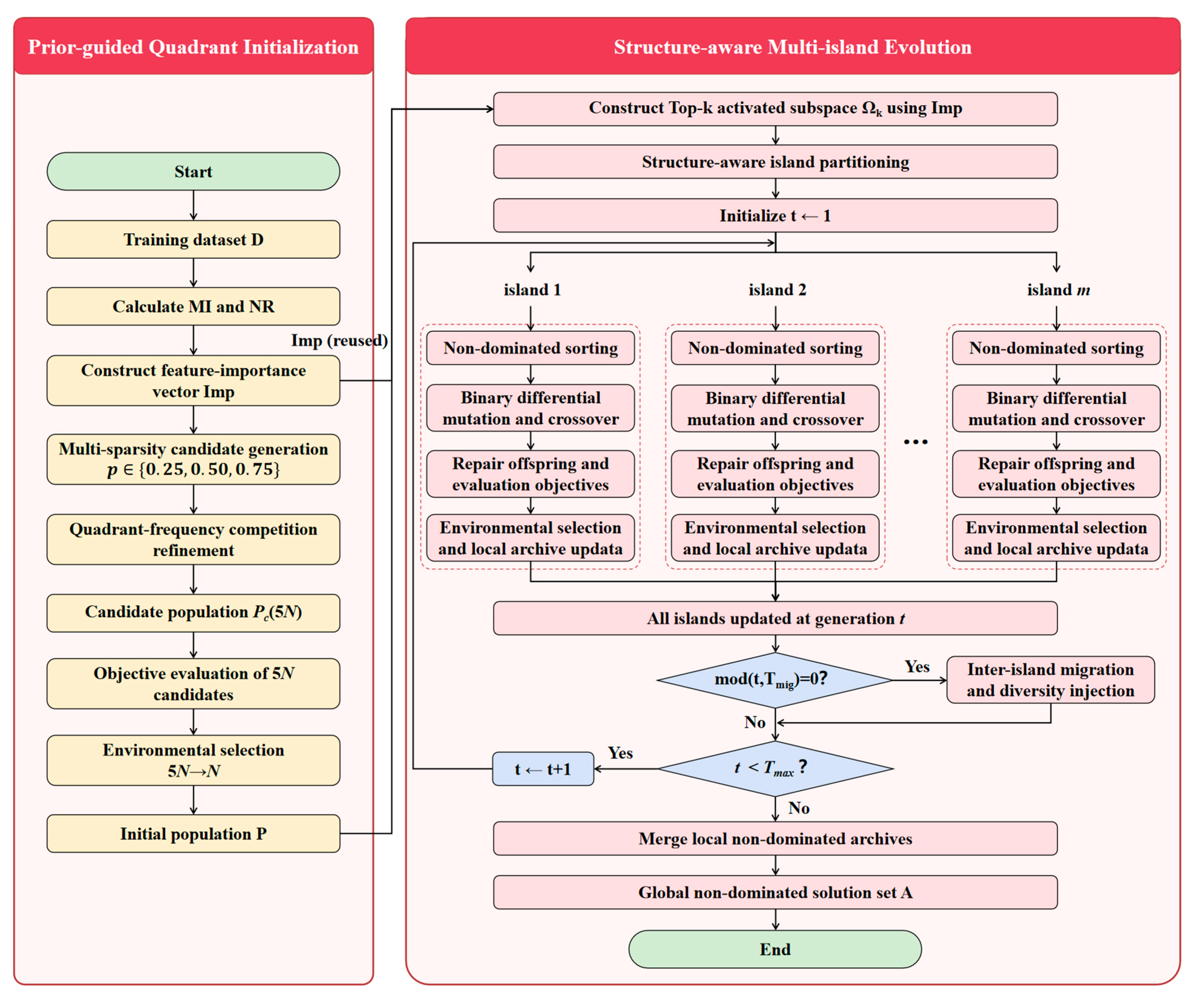
The overall procedure of PGS-MODE-FS is illustrated in Figure 1. Given a dataset, the algorithm first evaluates features from the perspectives of feature–class relevance and feature redundancy, and then uses the obtained feature importance information to support both population initialization and subsequent evolutionary search. Accordingly, PGS-MODE-FS is organized into two main stages: prior-guided quadrant initialization and structure-aware multi-island evolution. The former provides a high-quality initial population, while the latter organizes population structures and performs multi-objective evolutionary search. Through iterative evolution and environmental selection, PGS-MODE-FS finally obtains a set of non-dominated feature subsets with different trade-offs between classification performance and subset size.
The first stage is prior-guided quadrant initialization. For the training data, the algorithm first calculates feature relevance and feature redundancy, and then constructs a two-dimensional feature importance space accordingly. Based on this space, candidate feature subsets with different sparsity levels are generated, and their feature composition is further adjusted using a quadrant-frequency competition rule. After this process, a candidate population with a size of 5N and a comprehensive feature importance vector I m p are obtained. The candidate population is then evaluated according to the two optimization objectives and compressed by environmental selection to form the initial main population.
The second stage is structure-aware multi-island evolution. Based on the comprehensive feature importance vector I m p , the algorithm selects the Top-k activated features to define an informative subspace, in which the structural differences among individuals are measured. The population is then divided into multiple islands according to these structural differences. Within each island, binary differential evolution and environmental selection are performed independently to update the local population, while periodic migration provides limited information exchange among different islands. After iterative evolution, the algorithm outputs a set of non-dominated feature subsets. The detailed procedure is presented in Algorithm 1.
Algorithm 1 PGS-MODE-FS
Input: Training dataset D, population size N, maximum number of iterations T m a x , Top-k ratio η, island threshold τ, migration period T m i g
Output: Global non-dominated solution set A
1: ( P c , I m p ) Prior-guided Quadrant Initialization(D, 5N)     //Algorithm 2
2: Evaluate all individuals in P c using the two objective functions
3: P    E n v i r o n m e n t a l S e l e c t i o n ( P c , N)
4: A   M u l t i I s l a n d E v o l u t i o n (P, I m p , η, τ, T m a x , T m i g )     //Algorithm 3
5: return A

3.3. Prior-Guided Quadrant Initialization

The initial population serves as the starting point of multi-objective evolutionary search, and its quality and distribution directly affect the subsequent convergence speed and solution set quality. For high-dimensional feature selection problems, if initial individuals are generated entirely at random, the candidate subsets often contain a large number of features with weak discriminative ability or high redundancy. As a result, the algorithm may consume a considerable evaluation budget in the early stage to eliminate low-quality solutions. Conversely, if initialization relies only on a single importance ranking, a small number of high-scoring features tend to be repeatedly selected in the candidate population, leading to an overly concentrated initial structure and weakening the coverage of different sparsity levels and different error trade-off regions. To address this issue, this paper proposes a prior-guided quadrant initialization strategy which jointly exploits feature–class relevance information and redundancy information to generate an initial candidate population with improved quality and structural diversity.
To construct the prior information required for initialization, this paper characterizes feature utility from two complementary perspectives. First, mutual information (MI) [36] is adopted to measure the relevance between a feature and the class label. For the   j -th feature X j and the class variable C, mutual information is defined as
M I j = I X j ; C = x , c p ( x , c ) log p ( x , c ) p ( x ) p ( c ) .
A larger MIj indicates that the feature has a stronger statistical dependence on the class label and therefore provides greater feature–class relevance information. For the continuous-valued features considered in this study, mutual information is estimated using a nonparametric nearest-neighbor-based estimator with three nearest neighbors, without explicit discretization of the feature values. Second, to describe redundancy among features, the Pearson correlation coefficient [37] is used to measure the degree of linear correlation between any two features. For any two features X j and X l , the Pearson correlation coefficient is defined as
ρ X u , X v = c o v X u , X v σ u σ v .
Meanwhile, the overall redundancy level of the j -th feature is represented by the average absolute correlation coefficient between this feature and all the remaining features, namely,
R j = 1 D 1 k j ρ ( X j , X k ) ,
where D denotes the feature dimensionality. A larger Rj indicates that the j-th feature exhibits stronger average linear dependence with the remaining features and is therefore more likely to contain linearly redundant information. Since mutual information is positively associated with discriminative ability, whereas a lower redundancy level is preferred, the redundancy term is transformed into a same-direction indicator. Therefore, the non-redundancy score is defined as
N R j = 1 R j + ε   ,
where ε   = 10 8 is introduced to avoid numerical instability when R j approaches zero. Because MIj and NR j have different numerical ranges, both quantities are independently normalized to [0,1] using min-max normalization: M I J ~ = ( M I j m i n ( M I ) ) / ( m a x M I m i n M I ) ,   N R J ~ = ( N R j m i n N R ) / ( m a x N R m i n N R ) . The normalized discriminative and non-redundancy information are then integrated to construct the comprehensive importance index:
I m p j = λ · M I J ~ + μ · N R J ~ ,
where λ and μ are determined through the parameter sensitivity analysis described in Section 5.1 and are set to 0.7 and 0.3, respectively. This setting balances the use of feature–class relevance information and redundancy information during initialization, enabling the generated candidate solutions to retain informative features while reducing the influence of highly redundant ones.
Based on the normalized mutual information and non-redundancy scores, each feature is mapped onto a two-dimensional plane. An approximate minimum enclosing circle is then used to determine a reference center, according to which the features are divided into four quadrants, denoted as q, based on their relative positions. Considering that features with both high class relevance and low redundancy are more likely to form high-quality candidate subsets, this paper constructs a lightweight hierarchical rule: the first quadrant is preferred over the fourth quadrant, the fourth quadrant is preferred over the second quadrant, and the second quadrant is preferred over the third quadrant. Compared with global ranking based only on a single comprehensive score, this hierarchical strategy can preserve representative features from regions with different combinations of discriminability and redundancy during initialization, thereby alleviating the concentration effect caused by the repeated selection of high-scoring features.
Based on the above prior statistics and regional partitioning results, the proposed initialization strategy generates a candidate population under the guidance of the feature importance space. Let the main population size be N. To enlarge the initial coverage under a controllable computational cost, a candidate population with size M = 5N is generated. For each candidate solution, a sparsity threshold is first selected to form an initial feature subset, and the subset is then further adjusted according to the quadrant label, comprehensive importance value, and feature selection frequency. The detailed procedure is summarized in Algorithm 2.
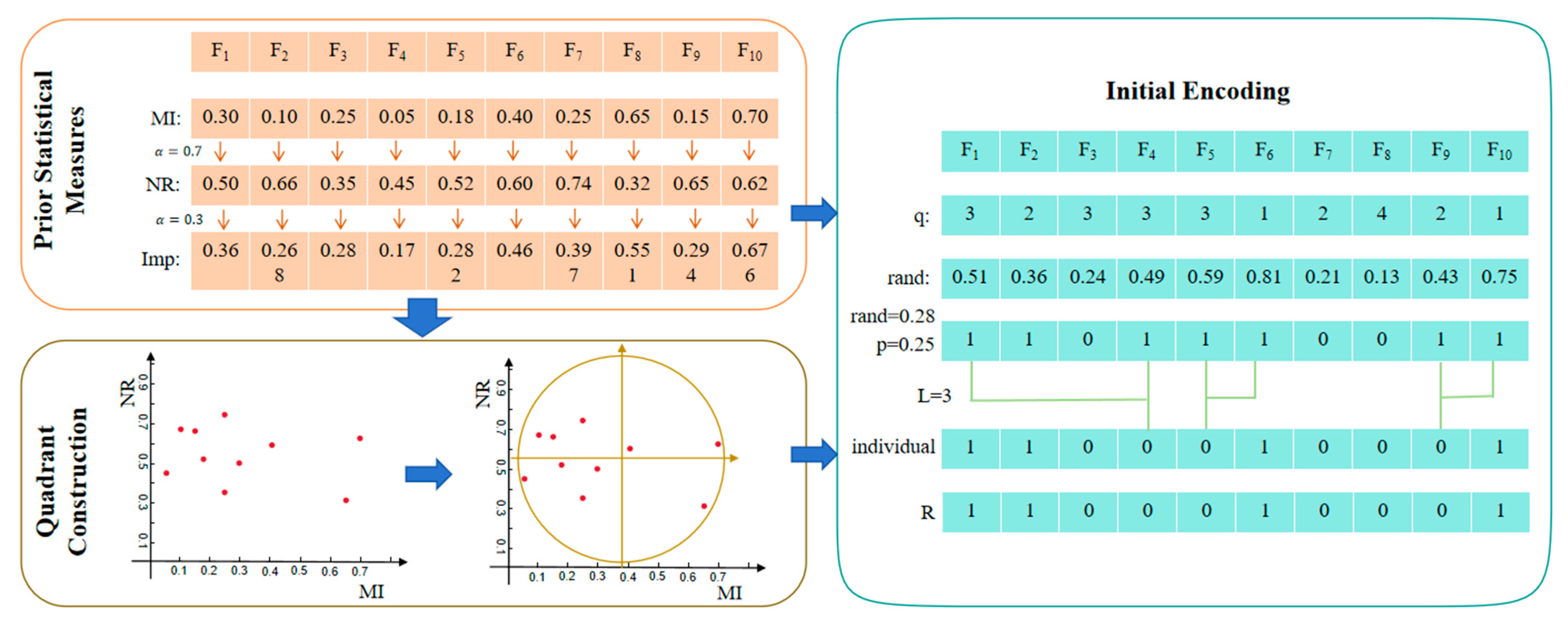
Since different thresholds correspond to different sparsity levels, this process can generate candidate solutions with different subset sizes, thereby preventing the initialized individuals from being concentrated in a single subset-size region. If an empty subset is produced after thresholding, the feature with the largest comprehensive importance value I m p is selected for repair, ensuring that each individual can be properly evaluated. After the initial subset is obtained, quadrant initialization further introduces a competition mechanism jointly driven by quadrant information and selection frequency to adjust the feature composition of the candidate solution. Specifically, when two competing features have the same cumulative selection frequency and belong to the same quadrant, the feature with a higher I m p value is preferentially retained to maintain the basic quality of the candidate solution. When they have the same frequency but belong to different quadrants, the selection is performed according to the quadrant preference rule, so as to preserve representative features from regions with different combinations of discriminability and redundancy. When their selection frequencies are different, the priority of the quadrant containing the high-frequency feature is decreased, giving the low-frequency feature a higher chance of being retained and thus suppressing the repeated selection of a small number of features during initialization. Through the joint effect of multi-sparsity thresholding, comprehensive importance constraints, and quadrant-frequency competition, the proposed initialization strategy can generate an initial population with a more reasonable distribution and stronger structural differences. For better illustration, Figure 2 uses 10 features as an example to demonstrate this process.
Taking the example in Figure 2, the normalized mutual information and non-redundancy score of each feature are first calculated to obtain the comprehensive importance value I m p . The features are then mapped into a two-dimensional importance space according to these two scores, and the quadrant label q of each feature is determined. During candidate solution generation, a random vector rand is generated, and preliminary feature selection is performed through a three-level thresholding scheme. In this example, the threshold is set to p = 0.25, producing the initial binary encoding [1,1,0,1,1,1,0,0,1,1]. The initial encoding is then refined through L pairwise competitions. Assuming L = 3, one competition randomly selects F1 and F4. Since both features belong to the third quadrant and have the same current selection frequency of 0, F1 is retained because it has a higher comprehensive importance value, whereas F4 is removed. This process is repeated until L comparisons are completed. Finally, the feature selection frequency vector R is updated according to the adjusted candidate solution.
Algorithm 2 Prior-guided Quadrant Initialization
Input: Training dataset D, candidate population size M = 5N
Output :   Candidate   population   P c   and   feature   importance   vector   I m p
1: Calculate MI and NR for all features according to Equations (5)–(8)
2: Calculate the comprehensive importance vector Imp according to Equation (9)
3: Map features into the MI-NR space and assign a quadrant label q to each feature
4: Initialize Pc ← empty and feature selection frequency vector R ← 0
5: for i = 1 to M do
6:    Select a sparsity threshold θ from {0.25, 0.50, 0.75}
7:    Generate an initial feature subset S according to θ
8:    if S is empty then
9:      Add the feature with the highest Imp value to S
10:  end if
11:  Refine S using the quadrant-frequency competition rule
12:  Encode S as a binary individual zi
13:  Update R according to zi
14:  PcPc ∪ {zi}
15:  end for
16:  return Pc and Imp

3.4. Structure-Aware Multi-Island Evolution Mechanism

The island model usually partitions the population into several relatively independent subpopulations and periodically exchanges individuals among them to maintain diversity and delay premature convergence [38,39,40]. However, in high-dimensional binary feature selection, directly measuring individual similarity in the full feature space can be easily disturbed by a large number of irrelevant and redundant features, making it difficult to accurately reflect the effective structural differences among individuals. Therefore, this paper uses the feature importance vector obtained from the initialization stage to construct a Top-k activated subspace, and measures individual differences only within this subspace. In this way, island partitioning can focus more on features with higher discriminative value and lower redundancy, thereby improving the effectiveness of population organization. Existing studies have shown that search space reduction, feature grouping, and feature importance-guided search are helpful for alleviating the search difficulty in high-dimensional feature selection [41,42,43]. The detailed procedure is summarized in Algorithm 3.
Based on the comprehensive feature importance vector obtained in Section 3.3, Imp   =   ( I m p 1 , I m p 2 , , I m p D ) , this paper selects the top k features with the highest scores to form an activation set, which is used to define the structural differences among individuals. The number of activated features is defined as
k = η · D ,
where η     ( 0 , 1 ) denotes the Top-k ratio parameter. According to the descending order of I m p , the top k features are selected to construct the activation set:
Ω k = T o p K I m p , k .
It should be noted that Ω k does not represent the final selected feature subset. Instead, it is used only to construct the activated subspace during island partitioning, so as to emphasize the structural differences among individuals on important feature dimensions.
Within the activated subspace, for any two individuals x i and x j , this paper adopts the normalized Hamming distance to measure their structural difference:
d H Ω k x i , x j = 1 k l Ω k Ι ( x i l x j l ) ,
where Ι · denotes the indicator function. Since the normalized Hamming distance is calculated over k activated features, its value lies in [0,1]. During incremental island partitioning, the distance between the current individual x and an existing island Ir is defined as
r ( x ) = m a x y I r   d H Ω k x , y .
Let C(x) = {r | ∆r(x) < τ, r = 1, 2,…, m} denote the set of eligible sub-islands for x, where τ is the island partitioning threshold. If C(x) ≠ ϕ, x is assigned to Ir*, where I r * = a r g   min r C ( x ) Δ r ( x ) . Otherwise, a new sub-island is created with x as its initial member. This maximum-distance criterion ensures that, during incremental assignment, x can enter an existing sub-island only when its normalized Hamming distance from every current member of that sub-island is smaller than τ. Therefore, a smaller τ imposes a stricter similarity requirement and generally produces more and smaller sub-islands, whereas a larger τ relaxes the requirement and generally produces fewer and more structurally heterogeneous sub-islands.
After the threshold-based partitioning is completed, a capacity-balancing procedure is applied to support the subsequent multi-island evolution. If only one sub-island is formed, a fallback split is performed to ensure that the multi-island mechanism is activated. The target capacity of each sub-island is then determined according to the total population size N and the current number of sub-islands. For over-capacity sub-islands, environmental selection is used for pruning, whereas under-capacity sub-islands are supplemented from the remaining candidate pool according to a distance-priority principle. This adjustment is performed after the threshold-based structural partitioning and is mainly used to maintain a reasonable population distribution among sub-islands.
In the present implementation, τ is not dynamically adapted during the evolutionary process. It is determined offline through the parameter sensitivity analysis described in Section 5.1. Once τ is selected, it remains fixed throughout all generations and is consistently used in all subsequent comparative and ablation experiments.
During the parallel evolutionary stage, each sub-island independently performs differential mutation, crossover, fitness evaluation, and environmental selection, while maintaining its own local non-dominated archive. Considering that individuals at different non-dominated ranks play different roles in the search process, this paper adopts two different binary differential mutation strategies according to the position of each individual in the current non-dominated sorting result. For individuals located on the current first non-dominated front, a random binary differential mutation strategy inspired by DE/rand/1/bin [44] is adopted:
V i , j = 1 X r 1 , j ,     i f    X r 2 , j   X r 3 , j   a n d   u j < F t X r 1 , j ,                   o t h e r w i s e                    j = 1 , 2 , 3 , , D ,
where Xr1, Xr2, and Xr3 are three randomly selected distinct individuals, with Xr1 serving as the base vector. u j ~ U ( 0 , 1 ) , and Ft denotes the scaling factor corresponding to the current iteration. This strategy mainly uses the structural differences among random individuals to perturb the front region, thereby enhancing structural dispersion near the Pareto front.
For individuals that do not belong to the current first non-dominated front, an advantage-guided binary mutation strategy inspired by DE/current-to-best/1/bin [45] is adopted:
V i , j = X b e s t , j ,                   i f   X b e s t , j X i , j   a n d   u 1 , j < F t   ,                                          1 X i , j ,    i f ( X b e s t , j = X i , j   o r   u i , j F t )   a n d   X r 1 , j X r 2 , j   a n d   u 2 , j < F t , X i , j ,                           o t h e r w i s e                                                                     j = 1 , 2 , 3 , , D ,
where Xi denotes the current individual, X b e s t denotes the best individual in the current island, Xr1 and Xr2 are two randomly selected distinct individuals, and u 1 , j , u 2 , j ~ U ( 0 , 1 ) . Based on preserving part of the structural information of the current individual, this strategy introduces information from the current superior individual to guide the update, thereby enhancing search directionality and improving subsequent convergence efficiency.
For the crossover operation, this paper adopts bitwise binary crossover [44] to generate the trial individual:
U i , j = V i , j ,      i f   u j   <   C R   o r   j = j r a n d , X i , j ,               o t h e r w i s e                         j = 1 , 2 , 3 , , D ,
where Xi denotes the parent individual, Vi denotes the mutation vector, CR denotes the crossover probability, and u j ~ U ( 0 , 1 ) . j r a n d is the forced crossover position, which ensures that at least one bit is inherited from the mutation vector, thereby preventing the trial individual from being identical to its parent. If the crossover result is an empty solution, one feature is randomly activated for repair to ensure that the individual can be evaluated.
Inter-island migration is performed every T m i g generations as an auxiliary information-exchange operation. A subset of representative non-dominated individuals from each island is migrated to neighboring islands, while a small number of randomly generated individuals are injected to avoid excessive aggregation in the later evolutionary stage. Following common settings in related studies, T m i g is set to 20 generations in this paper [46]. In this way, the proposed method maintains the connection between prior-guided initialization and structure-aware evolutionary search, thereby improving the coverage of different Pareto trade-off regions.
Algorithm 3 Structure-aware Multi-island Evolution
Input :   Initial   population   P ,   feature   importance   vector   I m p ,   Top - k   ratio   η ,   island   threshold   τ ,   maximum   number   of   iterations   T m a x ,   migration   period   T m i g
Output: Global non-dominated archive A
1: Construct the activated feature set Ω using the top k = ⌈ηD⌉ features in Imp
2: For each x  P, compute ∆r(x) for all existing islands; assign x to the eligible island with the smallest ∆r(x), or create a new island if no island satisfies ∆r(x) < τ .
3: Balance the capacity of each island by environmental selection or distance-priority supplementation
4: Initialize the local archive Ar for each island Ir
5: for t = 1 to Tmax do
6:   for each island Ir do
7:     Perform non-dominated sorting on Ir
8:     Generate offspring by binary differential mutation and crossover
9:     Repair invalid offspring and evaluate their objective values
10:       I r     E n v i r o n m e n t a l S e l e c t i o n ( I r     U r ,   N r )
11:       A r   N o n D o m i n a t e d S e l e c t i o n ( A r     I r )
12:    end for
13:    if mod ( t ,   T m i g ) = 0 then
14:      Perform inter-island migration and diversity injection
15:    end if
16:  end for
17:   A   N o n D o m i n a t e d S e l e c t i o n ( A 1     A 2       Am)
18:  return A
The computational cost of PGS-MODE-FS mainly includes prior-information calculation, candidate-population construction and evaluation, island partitioning, and multi-island evolution. Let M = 5N denote the number of initialization candidates, G the maximum number of generations, k = η D the number of activated features, and Ceval the cost of evaluating one candidate subset using five-fold KNN cross-validation. Calculating feature–class mutual information requires approximately O(nD) operations, whereas the exact all-pairs Pearson redundancy calculation requires O(nD2) time and O(D2) memory when a dense feature-correlation matrix is constructed. Candidate-population construction requires O(MD), while candidate evaluation requires O(MCeval). Constructing the Top-k activated feature set requires O(DlogD), and the worst-case incremental island-partitioning cost is O(N2k). During each generation, binary mutation and crossover require O(ND), candidate evaluation requires O(NCeval), and non-dominated sorting and environmental selection require up to O(N2). Therefore, the overall time complexity can be expressed as O ( n D 2 + M D + M C e v a l + D log D + N 2 k + G ( N D + N C e v a l + N 2 ) ) .
In addition to the above asymptotic complexity, the number of function evaluations (NFE) is further considered to quantify the actual evaluation budget under the adopted experimental settings. With N = 200 and G = 100, the 5N initialization candidates require 1000 evaluations, while the regular evolutionary process requires NG = 20,000 evaluations. Inter-island migration is performed every 20 generations. Migrated individuals retain their previously evaluated objective values and therefore do not require reevaluation; only newly generated diversity-injection individuals incur additional evaluations. Over 100 generations, five migration events are performed, introducing at most 100 additional evaluations. Therefore, the total NFE of PGS-MODE-FS ranges from 21,000 to 21,100.

4. Experimental Design

4.1. Dataset Description

To comprehensively evaluate the proposed method under datasets with different dimensional characteristics, 17 representative public and biomedical datasets were included, as summarized in Table 1. Their feature dimensionalities range from 13 to 10,000, covering a broad spectrum of feature-selection problems. Among them, six datasets—Wine, Australian, Zoo, Vehicle, WBCD, and Ionosphere—contain no more than 100 features and constitute the clearly lower-dimensional part of the benchmark suite, whereas the remaining 11 datasets contain between 166 and 10,000 features. The datasets also vary in class distribution, with Zoo, ST000419, Lung_discrete, and GQDL showing greater imbalance. Stratified partitioning and the balanced classification error rate were therefore used to reduce the influence of unequal class sizes.
In addition to the above public benchmark datasets, this paper also focuses on four datasets closely related to biomedical analysis, namely ST000385, ST000419, GQDL, and Leukemia. Overall, these datasets differ substantially in sample size, feature dimensionality, number of classes, and data complexity. They include not only public benchmark datasets suitable for general classification tasks, but also typical high-dimensional biomedical datasets. Therefore, they can provide a relatively comprehensive evaluation of the proposed method in terms of classification performance, feature reduction capability, and multi-objective search ability across different scenarios.

4.2. Experimental Settings

A unified data-partitioning, preprocessing, and evaluation procedure was adopted. For the comparative and ablation experiments, each algorithm was evaluated over 10 independent stratified holdout runs. In each run, the dataset was repartitioned into a training set and an independently held-out test set using an approximately 70/30 split, and the partition was regenerated across runs. Feature selection was performed exclusively on the training set. Candidate feature subsets were evaluated by five-fold stratified cross-validation within the training set using a K-nearest neighbor classifier with K = 5. Feature standardization was performed using z-score transformation, with the feature means and standard deviations estimated only from the training portion of each cross-validation fold and then applied unchanged to the corresponding held-out portion. After feature selection, the scaler and KNN classifier were refitted on the complete training set, and the fitted transformation was applied unchanged to the independently held-out test set for final performance assessment. For the parameter-sensitivity analysis, the same 70/30 stratified partitioning rule was adopted with 10 independent repetitions, while all candidate parameter settings were evaluated exclusively by five-fold stratified cross-validation within the training set.
The effectiveness of the proposed method is evaluated by comparing PGS-MODE-FS with six representative methods, including FPPFS [47], LMSSS [48], MOPSO-ASFS [49], NSGA-II [50], MODE_FDGM [51], and DMBDE [31]. FPPFS, LMSSS, and MOPSO-ASFS are representative multi-objective feature-selection methods employing different search strategies, while NSGA-II serves as a classical multi-objective evolutionary baseline. MODE_FDGM and DMBDE are differential-evolution-based multi-objective feature-selection methods and therefore provide more direct comparisons with PGS-MODE-FS in terms of evolutionary framework. DMBDE further incorporates a diversity-oriented mechanism to improve the distribution of candidate solutions in high-dimensional feature selection, providing a relevant comparison for the diversity-preservation aspect of PGS-MODE-FS.
The experimental results were analyzed from three perspectives: solution-set quality, convergence performance, and classification performance. To maintain consistent generation-based search settings, the population size and maximum number of generations were set to (N = 200) and (G = 100), respectively, for all algorithms. However, identical population sizes and generation limits do not necessarily imply identical numbers of fitness evaluations, because the compared methods differ in their initialization procedures and candidate-generation mechanisms. Therefore, the generation-based protocol was retained, while the actual evaluation schedules of all algorithms were further examined to make their computational budgets transparent. The resulting numbers of fitness evaluations, or rigorous lower and upper bounds when the exact counts were not fixed, are reported in Table S1 of the Supporting Information. All remaining algorithm-specific parameters were configured according to the corresponding original studies.
All experiments are conducted under the same hardware and software environment. The experimental platform is a 64-bit Windows operating system equipped with an Intel(R) Xeon(R) Platinum 8378C CPU @ 2.80 GHz and 16.0 GB of memory. All algorithms are implemented in Python 3.10. Because the training/test partition is regenerated for each run and the evolutionary search itself is stochastic, each algorithm was independently run 10 times on each dataset to reduce the influence of random variation. The final results are reported as the mean and standard deviation over the 10 independent runs.

4.3. Evaluation Metrics

In terms of evaluation, this paper assesses the algorithms from three aspects: solution set quality, convergence, and classification performance. Solution set quality is measured using the inverted generational distance (IGD) [52]. IGD is the inverse form of generational distance and is used to measure the average distance from the reference points on the true Pareto front to the non-dominated solution set obtained by an algorithm. However, the true Pareto front is unknown for the considered multi-objective feature-selection problems. Therefore, after all experimental runs had been completed, a reference Pareto front was constructed separately for each dataset. Specifically, the test-set nondominated objective vectors obtained by PGS-MODE-FS and all comparative algorithms over their 10 independently repeated stratified holdout runs were pooled into a unified set. Duplicate objective vectors were removed, and nondominated filtering was subsequently applied to the pooled set. Thus, the reference Pareto front summarized the complete repeated experimental procedure and was not constructed separately for each individual run. The IGD value was calculated separately for each algorithm in every run relative to this common reference front, and the resulting 10 IGD values were summarized as the mean and standard deviation. A smaller IGD value indicates that the solution set is closer to the reference Pareto front, implying better solution-set quality. The calculation formula of IGD is as follows:
I G D ( F * , F ) = 1 F * x F * m i n   d i s ( x ,   F ) ,
where F *   denotes the reference Pareto front, F denotes the Pareto front generated by the algorithm, F * denotes the number of solutions in the reference Pareto front, and min   dis ( x , F ) represents the minimum Euclidean distance from individual x to the individuals in F.
Algorithm convergence and diversity are measured using the hypervolume (HV) indicator [53]. The HV indicator was first proposed by Zitzler and Thiele. and represents the volume of the hypercube enclosed in the objective space by the solution set obtained by an algorithm and a given reference point. As an indicator that can simultaneously evaluate convergence and diversity, HV is currently one of the most reliable metrics for assessing multi-objective optimization algorithms, although it is highly sensitive to the choice of the reference point. Its evaluation principle is consistent with Pareto dominance: if a solution set S is superior to another solution set S1, then the HV value of S will also be larger than that of S1. The calculation formula is as follows:
H V ( F ) = Λ x F i = 1 m f i ( x ) , r i ,
where Λ   ( · )   denotes the Lebesgue measure, which is used to calculate volume. The subsequent part of the formula calculates the volume enclosed between each solution on the Pareto front and the reference point, while removing overlapping regions. The problem studied in this paper is a bi-objective minimization problem, where the two objectives correspond to the feature subset size and the classification error rate. Therefore, HV can be interpreted as the area covered by the non-dominated solution set and the reference point in the two-dimensional objective space. In this paper, the reference point for HV is uniformly set to (1.0, 1.0).
The minimum classification error rate (MCER) [47] was used to characterize the classification performance of a representative solution selected from the nondominated solution set, while the overall trade-off between classification error and feature subset size remained represented by the complete nondominated solution set and was assessed using the multi-objective performance indicators. Specifically, in each run, the solution with the minimum five-fold cross-validated balanced classification error rate among the training-stage nondominated solutions was selected as the representative solution. The corresponding feature subset was then evaluated once on the independently held-out test set, and the resulting balanced classification error rate was reported as the MCER of that run. Thus, the test set was used only for the final evaluation of the predefined representative solution rather than for its selection. A lower MCER value indicates better classification performance.

5. Experimental Results and Analysis

A series of experiments was conducted to evaluate the proposed PGS-MODE-FS method. Section 5.1 presents the parameter-sensitivity analysis and determines the default parameter settings. Section 5.2 compares PGS-MODE-FS with six representative multi-objective feature-selection methods in terms of HV, IGD, MCER, and computational cost. Section 5.3 reports the statistical analysis of the parameter and comparative results, including the corrected pairwise comparisons. Section 5.4 and Section 5.5 subsequently present the ablation study and further analyses of computational scalability and population diversity, respectively.

5.1. Analysis of Parameter Experimental Results

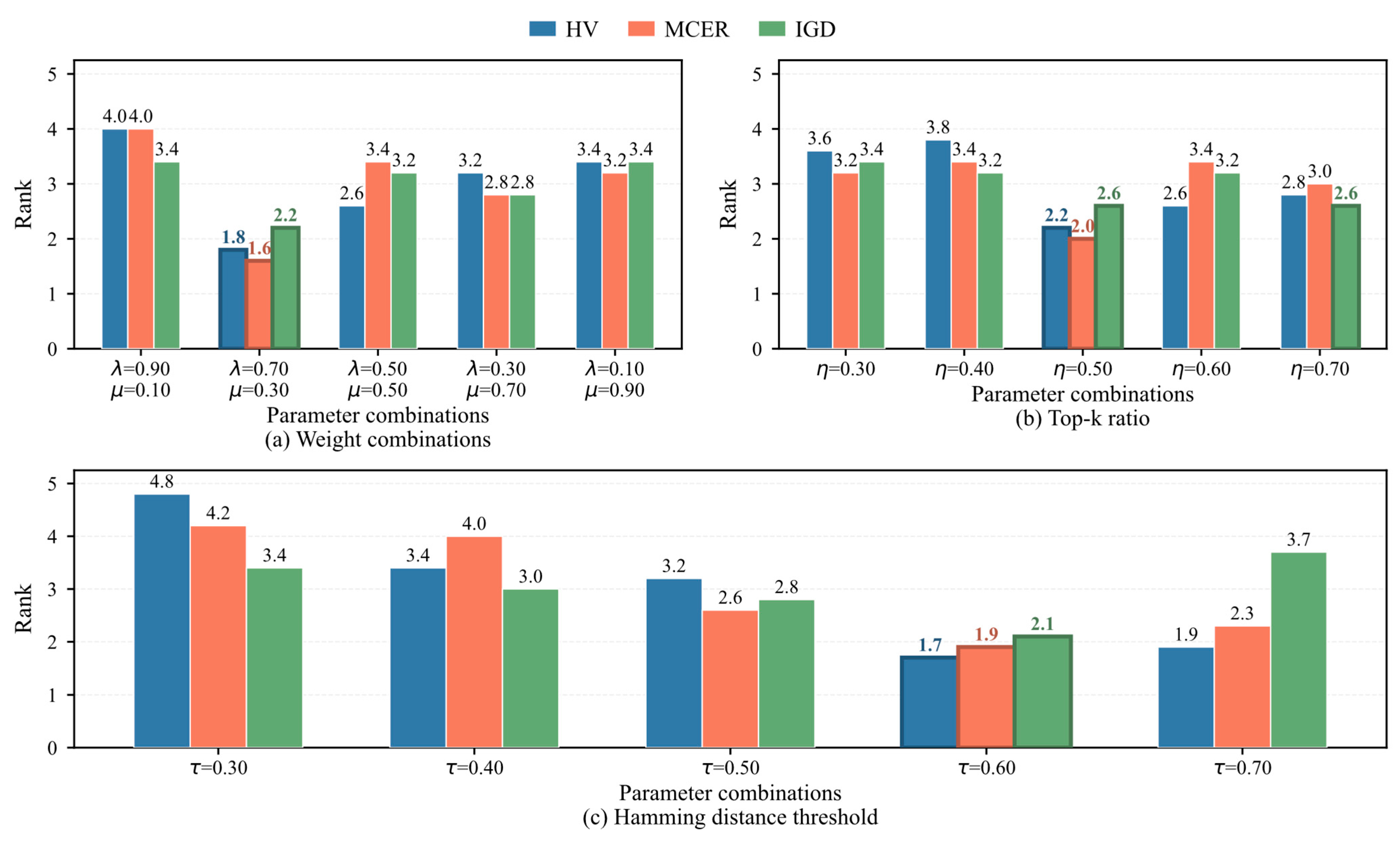
To determine the default values of the key parameters, sensitivity analyses were performed for the weight coefficients ( λ ,   μ ) , the Top-k activation ratio η , and the Hamming distance threshold τ using five representative datasets with different feature dimensionalities, namely Leukemia, ST000385, LSVT, Isolet, and WBCD. These datasets constitute a subset of the 17 benchmark datasets and therefore are not independent of the final benchmark at the dataset level. Parameter configurations were determined according to a composite ranking criterion integrating HV, IGD, and MCER. Specifically, for each metric, candidate settings were ranked on each dataset based on their mean performance over 10 independent repetitions. The resulting ranks were averaged across the five datasets, and the metric-specific average ranks were subsequently aggregated with equal weighting. The configuration yielding the lowest composite average rank was adopted as the default setting. For the calculation of IGD, the reference Pareto front was constructed solely from the nondominated solutions obtained during the training stage. The corresponding results are reported in Table 2, Table 3 and Table 4 and Figure 3.
Table 2 and Figure 3a show the sensitivity of PGS-MODE-FS to the weight coefficients ( λ ,   μ ) . The Friedman tests show no statistically significant overall differences among the five candidate settings for HV (p = 2.3108 × 10⁻¹), IGD (p = 7.2105 × 10⁻¹), or MCER (p = 1.7120 × 10⁻¹), indicating that the method is relatively stable over the examined weight combinations. Nevertheless, ( λ ,   μ ) = (0.70, 0.30) achieves the best average ranks for HV, IGD, and MCER, with values of 1.8000, 2.2000, and 1.6000, respectively. Its overall average rank across the three metrics is 1.8667, which is the lowest among the candidate settings. These results suggest that moderately emphasizing feature–class relevance while retaining the contribution of non-redundancy information provides a favorable balance across the three evaluation criteria. Therefore, ( λ ,   μ ) = (0.70, 0.30) is selected as the default setting.
Table 3 and Figure 3b show that the effect of the Top-k activation ratio η differs across the three evaluation metrics, and no consistent monotonic improvement is observed as η increases from 0.30 to 0.70. Among the five candidate values, η = 0.50 yields average ranks of 2.2000 for HV, 2.6000 for IGD, and 2.0000 for MCER. Although its advantage is not equally pronounced for every individual metric, these three ranks lead to the lowest combined average rank of 2.2667, indicating the best overall balance among solution-set quality, convergence, and classification performance. Meanwhile, the Friedman p-values for HV, IGD, and MCER are 4.5104 × 10⁻¹, 8.9109 × 10⁻¹, and 5.9607 × 10⁻¹, respectively, showing that the performance variation across the examined range is relatively moderate. Therefore, rather than favoring a particular metric, η = 0.50 is selected because it provides the most balanced overall performance among the candidate settings.
The influence of the Hamming distance threshold is shown in Table 4 and Figure 3c. Compared with the previous two parameters, τ has a more pronounced effect on HV. The Friedman test indicates a significant difference among the five threshold settings for HV (p = 1.2253 × 10⁻²), whereas the differences for IGD (p = 5.5277 × 10⁻¹) and MCER (p = 6.9421 × 10⁻²) are not statistically significant. Among the examined thresholds, τ = 0.60 obtains average ranks of 1.7000, 2.1000, and 1.9000 for HV, IGD, and MCER, respectively, resulting in the lowest combined average rank of 1.9000. The results show that increasing the threshold from relatively small values improves the overall ranking, but this advantage does not continue when the threshold is further enlarged. This pattern is consistent with the role of τ in island partitioning: a small threshold imposes a strict structural similarity requirement and may divide the population too finely, whereas an excessively large threshold weakens the separation among structurally different individuals. Therefore, τ = 0.60 provides a more appropriate partitioning granularity and is adopted as the fixed threshold in the subsequent experiments.
It can be seen that the proposed method exhibits good overall stability with respect to changes in key parameters. Based on the results of the parameter-sensitivity analysis, ( λ ,   μ ) = (0.70, 0.30), η = 0.50, and τ = 0.60 are finally adopted as the default settings for the subsequent experiments.

5.2. Comparison with Other Multi-Objective Feature Selection Methods

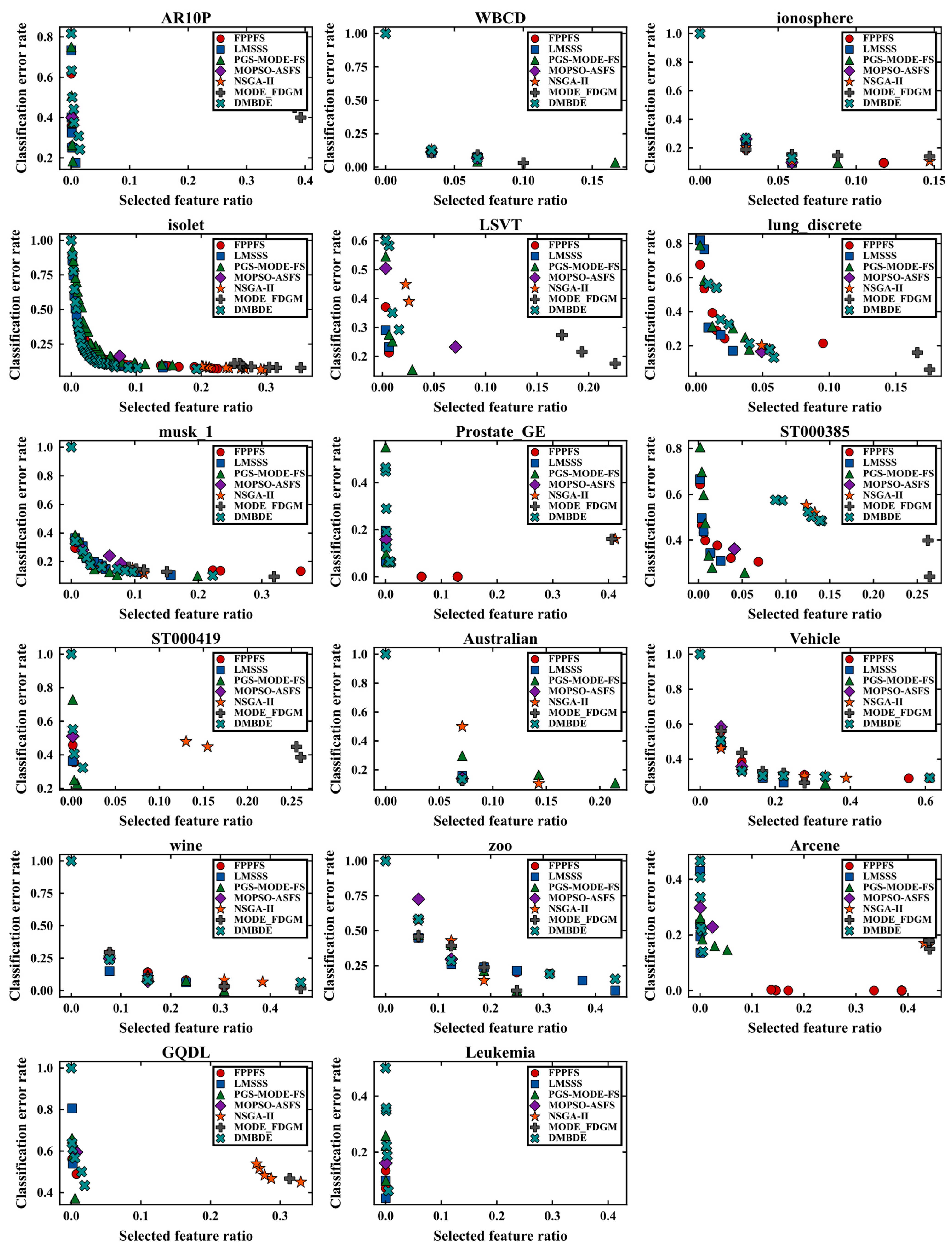
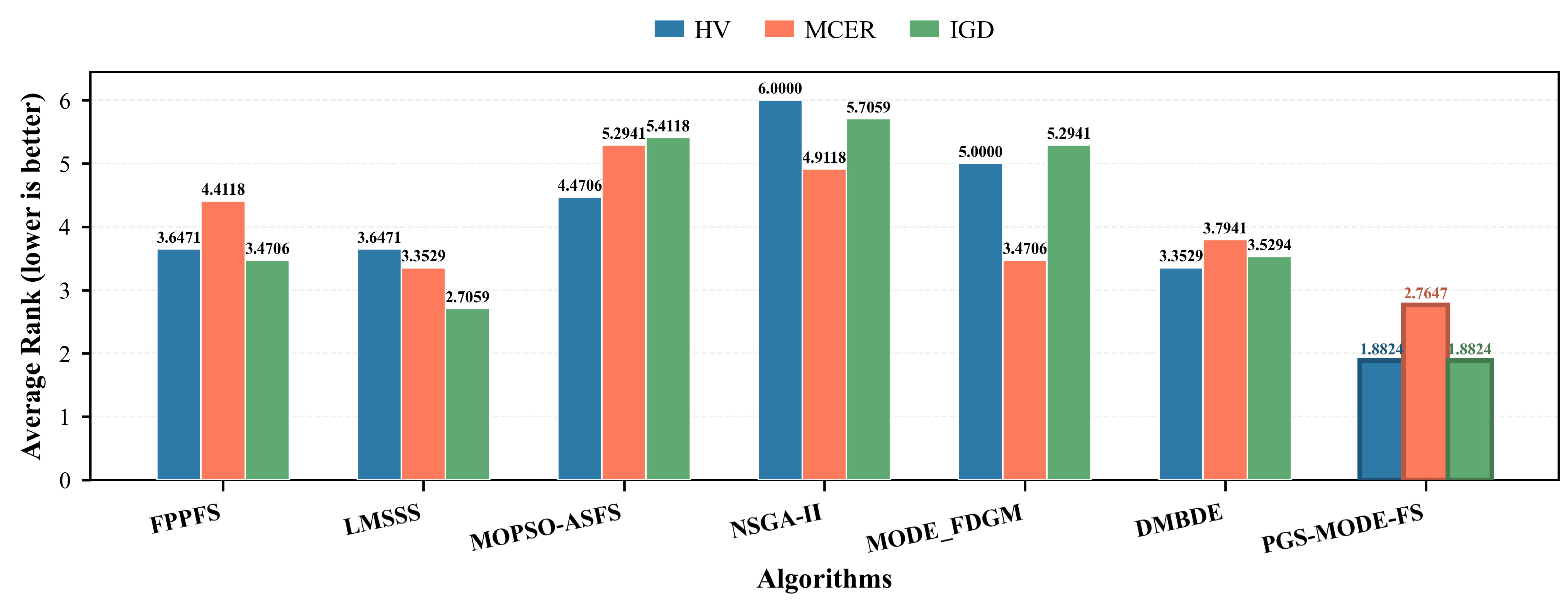
The proposed PGS-MODE-FS method is systematically compared with FPPFS, LMSSS, MOPSO-ASFS, NSGA-II, MODE_FDGM, and DMBDE on 17 datasets to evaluate its overall effectiveness. Table 5, Table 6 and Table 7 report the test results of the seven algorithms on HV, IGD, and MCER, respectively. Figure 4 further presents the distribution characteristics of the Pareto fronts on each dataset, while Figure 5 summarizes the overall performance of each method from the perspective of average ranks. The overall results show that PGS-MODE-FS achieves relatively better average ranks on multiple metrics, indicating that the proposed method obtains a good comprehensive balance among solution set quality, convergence stability, and classification performance.
From the perspective of multi-objective optimization performance, PGS-MODE-FS achieves the best descriptive average ranks for both HV in Table 5 and IGD in Table 6, with a value of 1.8824 for each metric. Although it does not obtain the best result on every dataset, it shows favorable overall performance across the benchmark suite. The Pareto fronts in Figure 4 further illustrate that PGS-MODE-FS can generate well-distributed nondominated solution sets and provide diverse trade-offs between classification error and feature-subset size.
The MCER results in Table 7 show that PGS-MODE-FS achieves the best descriptive average rank of 2.7647. It obtains the lowest or relatively low MCER values on multiple datasets, indicating competitive classification performance for the representative feature subsets selected by the proposed method. However, the average-rank result does not indicate whether PGS-MODE-FS significantly outperforms each comparative method. The corresponding cross-dataset statistical comparisons are therefore reported in Section 5.3.
The above comparisons summarize the overall performance across all 17 datasets. However, the benchmark suite spans a wide range of feature dimensionalities, including six datasets with no more than 100 features. To provide a more specific view of algorithm performance on datasets with larger feature spaces, the average ranks and Friedman statistics were additionally recalculated after excluding these six datasets. The results for the remaining 11 datasets are summarized in Table 8.
As shown in Table 8, PGS-MODE-FS achieves the best average ranks for both HV and IGD on the remaining 11 datasets, with values of 2.0000 and 2.0909, respectively. The corresponding Friedman tests remain statistically significant, with p = 3.2758 × 10⁻⁸ for HV and p = 1.1400 × 10⁻⁸ for IGD. These results indicate that PGS-MODE-FS maintains favorable Pareto-front coverage and approximation quality on datasets with larger feature spaces. For MCER, PGS-MODE-FS obtains an average rank of 3.3636, ranking second among the seven methods, while the Friedman test does not indicate a statistically significant overall difference (p = 0.0753). Thus, its classification performance remains competitive, although the relative advantage in MCER is less pronounced than that observed across the complete 17-dataset benchmark. Overall, the results on the D > 100 subset are consistent with the main conclusions obtained from the complete benchmark, particularly with respect to multi-objective optimization performance.
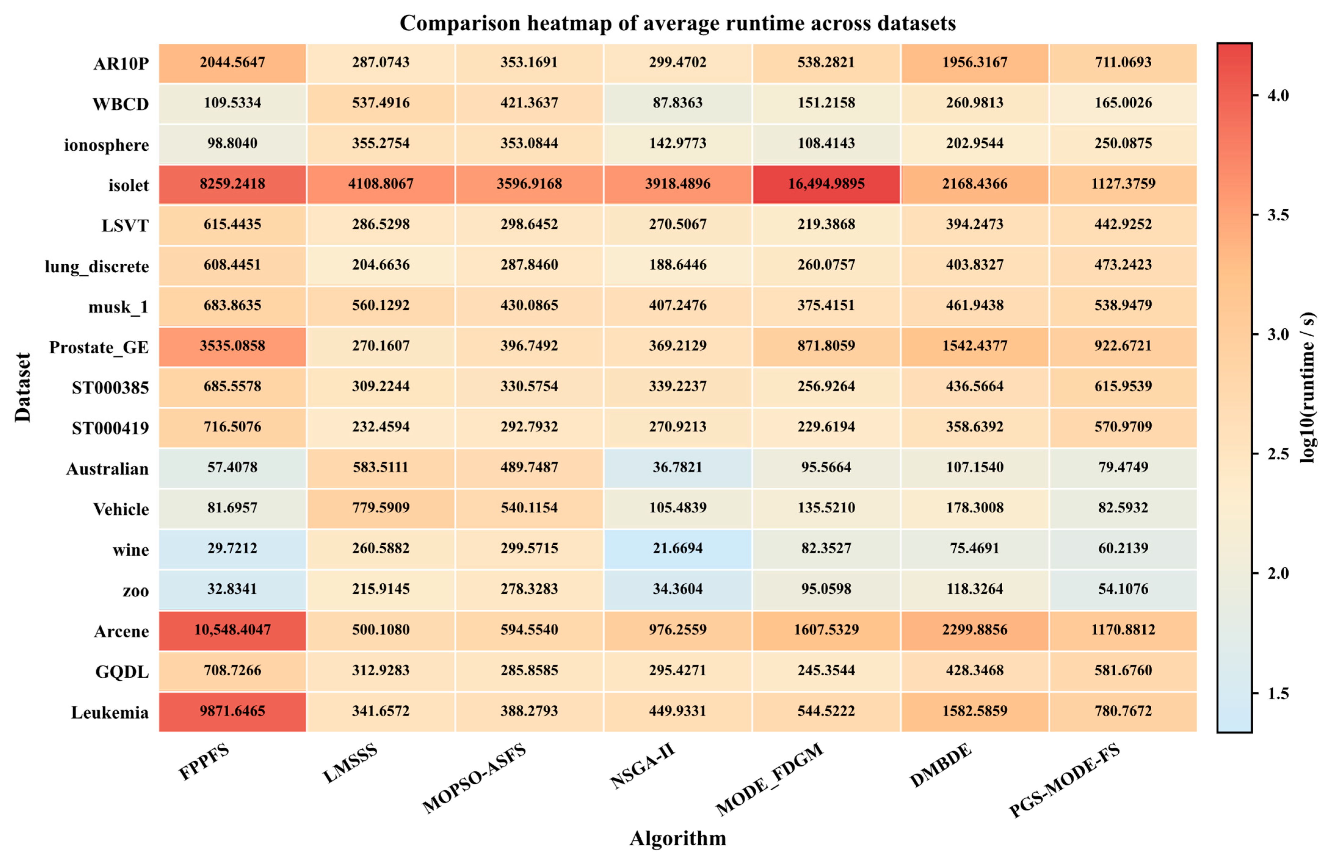
In addition to solution set quality and classification performance, running time is also an important indicator for evaluating the practical applicability of an algorithm. As shown in Table 9 and Figure 6, the running time of each algorithm generally increases with dataset size and feature dimensionality. Although PGS-MODE-FS does not achieve the shortest running time on all datasets, its average running time is lower than those of FPPFS, MOPSO-ASFS, MODE_FDGM, and DMBDE, and is comparable to that of NSGA-II. Combined with the results in Table 5, Table 6 and Table 7, PGS-MODE-FS shows a reasonable trade-off between computational cost and feature-selection performance. It should be noted, however, that computational practicality is application-dependent rather than determined by runtime alone. Studies of data-intensive IoT and smart-city systems have shown that practical computational methods must be considered together with application-specific requirements such as response time, resource utilization, scalability, and processing overhead [54,55]. From this perspective, the present results support the practicality of PGS-MODE-FS for the offline high-dimensional feature-selection tasks considered in this study, while its applicability to latency-critical or continuously updated environments would require further reduction in preprocessing and evolutionary-search costs.
Overall, Table 5, Table 6, Table 7, Table 8 and Table 9 and Figure 4, Figure 5 and Figure 6 show that PGS-MODE-FS achieves a good balance among Pareto front coverage, approximation quality, classification performance, and computational cost. These results are consistent with the unified design of the proposed method. The prior-guided initialization improves the starting distribution by introducing discriminative and non-redundant feature information, while the structure-aware multi-island evolution continues to use the same information to organize diverse search regions. Therefore, the performance gain is not attributed to isolated operators, but to the continuous use of feature prior information across initialization and evolution.

5.3. Statistical Analysis

The preceding comparisons describe the central tendency and overall ranking of the algorithms, but they do not by themselves establish whether the observed differences are statistically reliable. Therefore, statistical comparisons were conducted at both the individual-dataset and cross-dataset levels. At the individual-dataset level, the run-level results of each non-reference method or parameter setting were compared with those of the designated reference using a two-sided Mann–Whitney U test. Holm’s step-down procedure was applied separately within each dataset and metric to correct four parameter-setting comparisons in Table 2, Table 3 and Table 4 and six comparator-versus-PGS-MODE-FS comparisons in Table 5, Table 6 and Table 7. At a significance level of 0.05, “+”, “−”, and “≈” indicate that the non-reference method or setting is significantly better than, significantly worse than, or not significantly different from the designated reference after Holm correction, respectively. Thus, the symbols and the corresponding win/loss/tie counts in Table 2, Table 3, Table 4, Table 5, Table 6 and Table 7 represent corrected within-dataset comparisons.
Because these within-dataset comparisons do not determine whether an algorithm exhibits a consistent overall advantage across the complete benchmark suite, the dataset-level mean results were further analyzed using the Friedman test. The Friedman tests indicated significant overall differences among the seven algorithms for HV (p = 1.2347 × 10⁻⁶), IGD (p = 1.0645 × 10⁻⁸), and MCER (p = 6.1694 × 10⁻³). However, the Friedman test is an omnibus test and does not identify which specific algorithm pairs differ significantly. Therefore, PGS-MODE-FS was subsequently compared with each of the six comparative algorithms using a two-sided Wilcoxon signed-rank test, followed by Holm correction. The resulting adjusted p-values and comparison outcomes are summarized in Table 10.
As shown in Table 10, PGS-MODE-FS significantly outperforms FPPFS, MOPSO-ASFS, NSGA-II, and MODE-FDGM for both HV and IGD after Holm correction. Its differences from LMSSS and DMBDE are not statistically significant for either metric. For MCER, PGS-MODE-FS significantly outperforms MOPSO-ASFS and NSGA-II, whereas its differences from FPPFS, LMSSS, MODE-FDGM, and DMBDE are not statistically significant. These results provide statistical support for part of the average-rank advantages observed in Table 5, Table 6 and Table 7, while also showing that PGS-MODE-FS does not significantly outperform every comparative algorithm.
Accordingly, average ranks are used only as descriptive summaries of the overall performance ordering, whereas claims of statistical superiority are restricted to the algorithm pairs supported by the Holm-adjusted comparisons. To further characterize the uncertainty of the mean results, two-sided 95% confidence intervals were calculated using Student’s t distribution. The corresponding confidence intervals for HV, IGD, and MCER are reported in Tables S2–S4 of the Supporting Information, respectively.

5.4. Ablation Study

To analyze the influence of the key components on algorithm performance, two ablation variants are designed in this paper. RI-MODE-FS replaces the prior-guided quadrant initialization with random initialization to examine the effect of the initial population structure. SP-MODE-FS retains the proposed initialization strategy but removes the Top-k activation-based multi-island organization mechanism and adopts single-population evolution instead, so as to verify the role of structure-aware multi-island evolutionary search. Except for these module differences, all other experimental settings are kept the same. As shown in Table 11 and Table 12, the complete PGS-MODE-FS obtains the best average ranks on HV, MCER, and IGD, with values of 1.1176, 1.4118, and 1.1765, respectively, and the Friedman test results are statistically significant for all three metrics. These results indicate that both prior-guided quadrant initialization and structure-aware multi-island evolutionary search contribute positively to the performance improvement. They play complementary roles in improving the initial search distribution and maintaining population diversity during evolution.
Compared with RI-MODE-FS, the complete method shows more stable advantages on HV and IGD, indicating that prior-guided initialization helps improve the coverage and convergence performance of the non-dominated solution set. Without prior guidance, random initialization may generate low-quality candidate solutions or candidate solutions with similar structures, which weakens the subsequent search. In contrast, the proposed initialization stage provides a more informative and structurally diverse starting distribution.
The results of SP-MODE-FS further demonstrate the necessity of continuing the same structural guidance during evolution. Although prior-guided initialization improves the initial population, single-population evolution is still prone to structural aggregation as the search proceeds. By constructing a Top-k activated subspace from the same feature importance vector and organizing individuals into multiple islands, PGS-MODE-FS can better preserve different feature-subset structures and improve the distribution quality of the Pareto solution set. This confirms that the two stages are complementary rather than simply stacked.

5.5. Further Analysis

To further evaluate PGS-MODE-FS beyond the final performance metrics, two complementary analyses were conducted, focusing on the computational scalability of redundancy estimation and the population diversity behavior of the structure-aware multi-island mechanism. Detailed experimental settings and metric definitions are provided in Sections S3 of the Supporting Information.
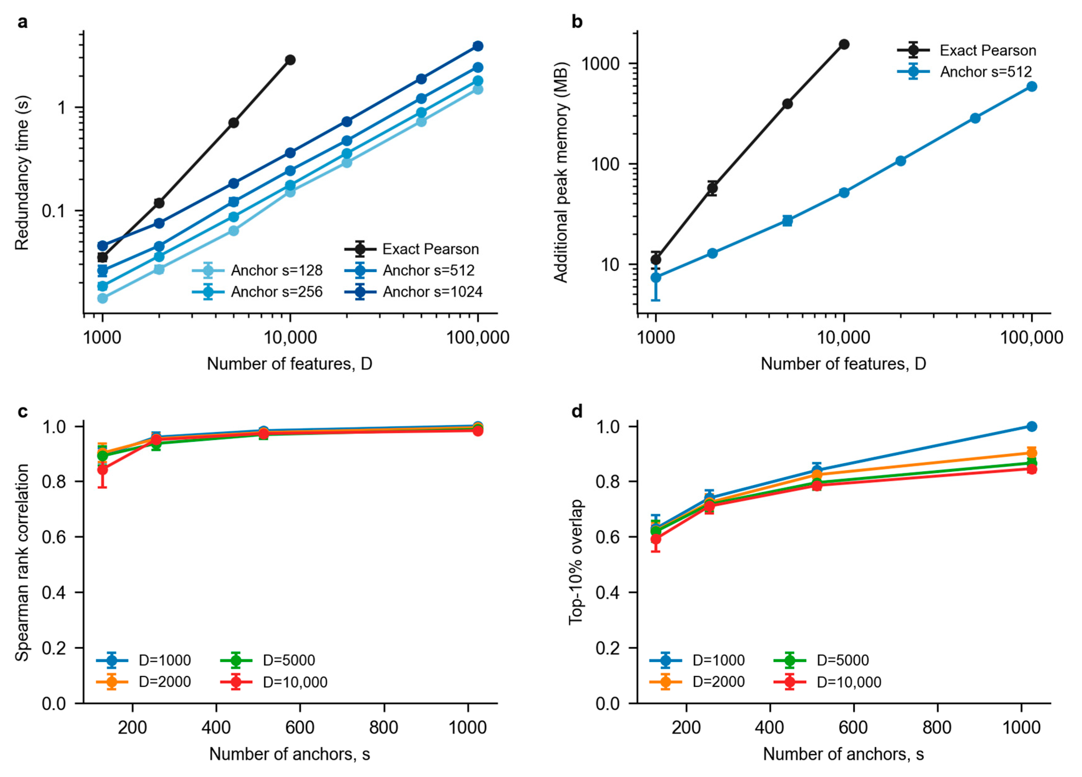
From the perspective of computational scalability, Figure 7 shows that the sampled-anchor approximation substantially reduced the runtime and memory requirements of redundancy estimation as feature dimensionality increased, while maintaining high agreement with the exact redundancy ranking. At 10,000 features, the 512-anchor approximation achieved a Spearman correlation of 0.9728 ± 0.0063 with the exact ranking while reducing redundancy-estimation time from 2.849 ± 0.129 s to 0.243 ± 0.009 s. As further summarized in Table S5 of the Supporting Information, results on three high-dimensional datasets showed more than tenfold reductions in redundancy-estimation time, although the total runtime changed only slightly because evolutionary search remained the dominant computational cost. This result also highlights a computational trade-off in redundancy-aware representation: suppressing redundant variables can provide a more informative basis for subsequent search, but constructing the redundancy representation itself introduces preprocessing cost, which must be controlled in ultra-high-dimensional settings.
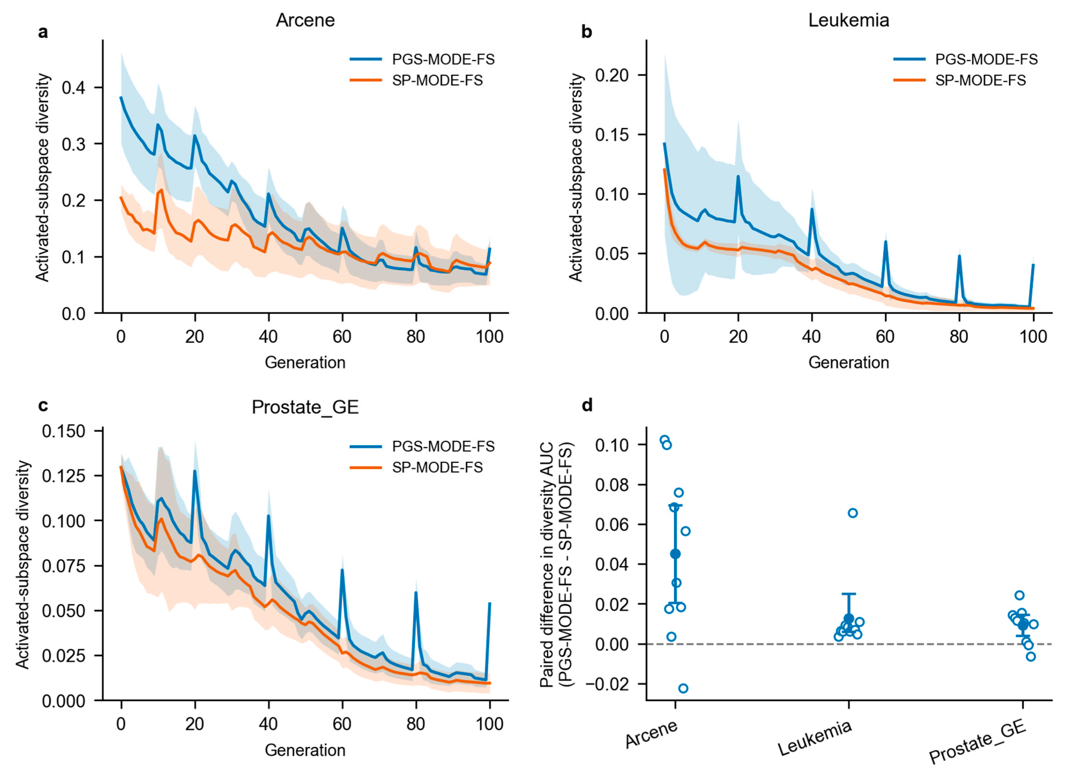
From the perspective of population diversity, Figure 8 shows that PGS-MODE-FS generally maintained higher activated-subspace diversity than SP-MODE-FS on Arcene, Leukemia, and Prostate_GE. Diversity periodically recovered around the migration generations, indicating that inter-island information exchange helped alleviate population aggregation. The normalized diversity AUC was increased by approximately 37.5%, 42.9%, and 20.1% on the three datasets, respectively, with statistically significant paired differences after Holm correction (Table S6 in the Supporting Information). These results provide additional evidence for the diversity-maintenance role of the structure-aware multi-island mechanism.
Overall, these additional analyses complement the endpoint comparative and ablation results by further characterizing the computational boundary of exact redundancy estimation and the diversity-maintenance behavior of the proposed multi-island mechanism.

6. Conclusions

This paper proposed PGS-MODE-FS to address the challenges of low-quality initialization and population aggregation in high-dimensional multi-objective feature selection. The method employs a unified feature importance representation to guide both candidate-population construction and structure-aware multi-island evolution. Experiments on 17 public and biomedical datasets demonstrated competitive overall performance in terms of solution-set quality, classification performance, feature reduction, and computational cost. In addition, the dimensionality-stratified analysis showed that PGS-MODE-FS retained the best average ranks for HV and IGD after the six lower-dimensional datasets were excluded, providing further support for its multi-objective search capability on datasets with larger feature spaces. The population diversity analysis also showed that PGS-MODE-FS maintained higher activated-subspace diversity than its single-population variant on Arcene, Leukemia, and Prostate_GE. Moreover, the observed separation between within-island and between-island distances further supported the role of island partitioning in preserving structural diversity.
The study also identified a computational limitation of exact redundancy estimation. Although the exact all-pairs Pearson calculation remained feasible for the benchmark dimensionalities considered in this study, its quadratic growth in computational and memory requirements may restrict direct application to substantially higher-dimensional data. The sampled-anchor approximation substantially reduced the cost of redundancy estimation while retaining high agreement with the exact redundancy ranking. However, the 100,000-feature experiment evaluated the redundancy-estimation stage rather than the complete evolutionary procedure. Future work will therefore investigate more scalable redundancy-estimation strategies, end-to-end validation on ultra-high-dimensional datasets, and adaptive control of the evolutionary parameters.

Supplementary Materials

The following supporting information can be downloaded at: https://www.mdpi.com/article/10.3390/a19090797/s1, Table S1: Source-code-derived exact numbers or bounds of objective-function evaluations under N = 200 and G = 100; Table S2: Mean and 95% confidence intervals of HV obtained by the seven algorithms; Table S3: Mean and 95% confidence intervals of IGD obtained by the seven algorithms; Table S4: Mean and 95% confidence intervals of MCER obtained by the seven algorithms; Table S5: Runtime and descriptive performance comparison between the exact PGS-MODE-FS and the sampled-anchor variant with s = 512 on three high-dimensional datasets. Values are reported as the mean ± standard deviation over 10 runs. Exact/Anchor denotes the exact version followed by the sampled-anchor version; Table S6: Activated-subspace diversity AUC of PGS-MODE-FS and SP-MODE-FS over 10 paired runs. Values for each method are reported as the mean ± standard deviation. Confidence intervals are 95% bootstrap confidence intervals for the paired mean difference. The reported p-values were obtained using two-sided Wilcoxon signed-rank tests followed by Holm correction across the three datasets.

Author Contributions

Conceptualization, J.D.; methodology, G.H., J.L., T.W., Q.H. and J.D.; software, J.D.; validation, G.H., J.H., H.L., Z.L. and J.C.; formal analysis, J.L. and J.D.; investigation, G.H.; resources, T.W. and Q.H.; data curation, J.H., H.L., Z.L. and J.C.; writing—original draft preparation, G.H.; writing—review and editing, J.D.; supervision, J.D. All authors have read and agreed to the published version of the manuscript.

Funding

This research was funded by the National Natural Science Foundation of China, grant numbers 82260988, 82160955, and 82274680; the “Science and Technology + Traditional Chinese Medicine” Project of Jiangxi Province, grant number 2023KZI01004; the Key Research and Development Program of Jiangxi Province, grant number 20243BCC31011; the Science and Technology Research Project of the Jiangxi Provincial Department of Education, grant number GJJ211256; the Science and Technology Program of the Jiangxi Administration of Traditional Chinese Medicine, grant number 2024B0736; and The APC was funded by the National Natural Science Foundation of China, grant number 82260988.

Data Availability Statement

The codes used in this study are publicly available at https://github.com/kaldks/PGS-MODE-FS (accessed on 14 September 2026), and can be used to reproduce the results reported in this paper.

Conflicts of Interest

The authors declare no competing interests.

References

  1. Pudjihartono, N.; Fadason, T.; Kempa-Liehr, A.W.; O’Sullivan, J.M. A review of feature selection methods for machine learning-based disease risk prediction. Front. Bioinform. 2022, 2, 927312. [Google Scholar] [CrossRef] [Scilit]
  2. Salhi, A.; Alshamrani, R.; Althbiti, A.; Ismail, A.; Abd-ElRahman, M.; Hassan, B.M. Optimizing high dimensional data classification with a hybrid AI driven feature selection framework and machine learning schema. Sci. Rep. 2025, 15, 35038. [Google Scholar] [CrossRef] [Scilit]
  3. Saeys, Y.; Inza, I.; Larrañaga, P. A review of feature selection techniques in bioinformatics. Bioinformatics 2007, 23, 2507–2517. [Google Scholar] [CrossRef] [Scilit]
  4. Malekipirbazari, M.; Aksakalli, V.; Shafqat, W.; Eberhard, A. Performance comparison of feature selection and extraction methods with random instance selection. Expert Syst. Appl. 2021, 179, 115072. [Google Scholar] [CrossRef] [Scilit]
  5. Xue, B.; Fu, W.; Zhang, M. Multi-objective feature selection in classification: A differential evolution approach. In Simulated Evolution and Learning; Dick, G., Browne, W.N., Whigham, P., Zhang, M., Bui, L.T., Ishibuchi, H., Jin, Y., Li, X., Shi, Y., Singh, P., et al., Eds.; Springer International Publishing: Cham, Switzerland, 2014; pp. 516–528. [Google Scholar] [CrossRef] [Scilit]
  6. Jagdhuber, R.; Rahnenführer, J. Implications on feature detection when using the benefit–cost ratio. SN Comput. Sci. 2021, 2, 316. [Google Scholar] [CrossRef] [Scilit]
  7. Jiao, R.; Nguyen, B.H.; Xue, B.; Zhang, M. A survey on evolutionary multiobjective feature selection in classification: Approaches, applications, and challenges. IEEE Trans. Evol. Comput. 2024, 28, 1156–1176. [Google Scholar] [CrossRef] [Scilit]
  8. Xue, Y.; Cai, X.; Neri, F. A multi-objective evolutionary algorithm with interval based initialization and self-adaptive crossover operator for large-scale feature selection in classification. Appl. Soft Comput. 2022, 127, 109420. [Google Scholar] [CrossRef] [Scilit]
  9. Miyandoab, S.Z.; Rahnamayan, S.; Bidgoli, A.A.; Ebrahimi, S.; Makrehchi, M. Enhancing diversity in multi-objective feature selection. In Proceedings of the 2024 IEEE Congress on Evolutionary Computation (CEC), Yokohama, Japan, 30 June–5 July 2024; pp. 1–8. [Google Scholar] [CrossRef] [Scilit]
  10. Feng, Y.; Feng, L.; Liu, S.; Kwong, S.; Tan, K.C. Towards multi-objective high-dimensional feature selection via evolutionary multitasking. Swarm Evol. Comput. 2024, 89, 101618. [Google Scholar] [CrossRef] [Scilit]
  11. Dong, H.; Sun, J.; Sun, X. A multi-objective multi-label feature selection algorithm based on Shapley value. Entropy 2021, 23, 1094. [Google Scholar] [CrossRef] [Scilit]
  12. Rafie, A.; Moradi, P.; Ghaderzadeh, A. A multi-objective online streaming multi-label feature selection using mutual information. Expert Syst. Appl. 2023, 216, 119428. [Google Scholar] [CrossRef] [Scilit]
  13. Yu, K.; Sun, S.; Liang, J.; Chen, K.; Qu, B.; Yue, C.; Wang, L. A bidirectional dynamic grouping multi-objective evolutionary algorithm for feature selection on high-dimensional classification. Inf. Sci. 2023, 648, 119619. [Google Scholar] [CrossRef] [Scilit]
  14. Kost, L.; Lier, S.K.; Breitner, M.H. An explainable artificial intelligence feature selection framework for transparent, trustworthy, and cost-efficient energy forecasting. Energy AI 2025, 22, 100648. [Google Scholar] [CrossRef] [Scilit]
  15. Wang, Y.; Lier, S.K.; Li, F.; Maier, S.; Oestreich, T.; Breitner, M.H.; Schade, W. An explainable artificial intelligence-based feature engineering strategy for lightweight battery health estimation. J. Energy Storage 2026, 155, 121444. [Google Scholar] [CrossRef] [Scilit]
  16. Ferraz-Caetano, J.; Teixeira, F.; Cordeiro, M.N.D.S.; Miyao, T. Inverse ligand design: A generative data-driven model for optimizing vanadyl-based epoxidation catalysts. J. Catal. 2026, 453, 116537. [Google Scholar] [CrossRef] [Scilit]
  17. Xue, B.; Fu, W.; Zhang, M. Differential evolution (DE) for multi-objective feature selection in classification. In Proceedings of the Companion Publication of the 2014 Annual Conference on Genetic and Evolutionary Computation, Vancouver, BC, Canada, 12–16 July 2014; pp. 83–84. [Google Scholar] [CrossRef] [Scilit]
  18. Sikdar, U.K.; Ekbal, A.; Saha, S. MODE: Multiobjective differential evolution for feature selection and classifier ensemble. Soft Comput. 2015, 19, 3529–3549. [Google Scholar] [CrossRef] [Scilit]
  19. Xu, H.; Xue, B.; Zhang, M. Segmented initialization and offspring modification in evolutionary algorithms for bi-objective feature selection. In Proceedings of the 2020 Genetic and Evolutionary Computation Conference, Cancún, Mexico, 8–12 July 2020; pp. 444–452. [Google Scholar] [CrossRef] [Scilit]
  20. Chen, C.; Yao, X.; Gong, D.; Tu, H. A multi-objective evolutionary algorithm for feature selection incorporating dominance-based initialization and duplication analysis. Swarm Evol. Comput. 2025, 95, 101914. [Google Scholar] [CrossRef] [Scilit]
  21. Pan, H.; Chen, S.; Xiong, H. A high-dimensional feature selection method based on modified Gray Wolf Optimization. Appl. Soft Comput. 2023, 135, 110031. [Google Scholar] [CrossRef] [Scilit]
  22. Wang, P.; Xue, B.; Liang, J.; Zhang, M. Multiobjective differential evolution for feature selection in classification. IEEE Trans. Cybern. 2023, 53, 4579–4593. [Google Scholar] [CrossRef] [Scilit]
  23. Dominico, G.; Bernardes, J.S.; Dorneles, L.L.; Dorn, M. Multi-objective wrapper differential evolution with guided initial population for feature selection. In Proceedings of the 2023 IEEE Congress on Evolutionary Computation (CEC), Chicago, IL, USA, 1–5 July 2023; pp. 1–8. [Google Scholar] [CrossRef] [Scilit]
  24. Yu, F.; Guan, J.; Wu, H.; Wang, H.; Ma, B. Multi-population differential evolution approach for feature selection with mutual information ranking. Expert Syst. Appl. 2025, 260, 125404. [Google Scholar] [CrossRef] [Scilit]
  25. Zhang, Z.; An, Q.; Wang, Y.; Wu, C.; Dong, B.; Zhou, C. Enhanced differential evolution for high-dimensional feature selection. J. King Saud Univ. Comput. Inf. Sci. 2026, 38, 270. [Google Scholar] [CrossRef] [Scilit]
  26. Li, M.; Zhao, Y.; Cao, R.; Wang, J.; Wu, D. A recursive framework for improving the performance of multi-objective differential evolution algorithms for gene selection. Swarm Evol. Comput. 2024, 87, 101546. [Google Scholar] [CrossRef] [Scilit]
  27. Zhang, Y.; Gong, D.; Gao, X.; Tian, T.; Sun, X. Binary differential evolution with self-learning for multi-objective feature selection. Inf. Sci. 2020, 507, 67–85. [Google Scholar] [CrossRef] [Scilit]
  28. Pan, J.S.; Liu, N.; Chu, S.C. A competitive mechanism based multi-objective differential evolution algorithm and its application in feature selection. Knowl.-Based Syst. 2022, 245, 108582. [Google Scholar] [CrossRef] [Scilit]
  29. Yu, X.; Hu, Z.; Luo, W.; Xue, Y. Reinforcement learning-based multi-objective differential evolution algorithm for feature selection. Inf. Sci. 2024, 661, 120185. [Google Scholar] [CrossRef] [Scilit]
  30. Nayak, S.K.; Rout, P.K.; Jagadev, A.K.; Swarnkar, T. Elitism-based multi-objective differential evolution with extreme learning machine for feature selection: A novel searching technique. Connect. Sci. 2018, 30, 362–387. [Google Scholar] [CrossRef] [Scilit]
  31. Wang, P.; Xue, B.; Liang, J.; Zhang, M. Feature selection using diversity-based multi-objective binary differential evolution. Inf. Sci. 2023, 626, 586–606. [Google Scholar] [CrossRef] [Scilit]
  32. Wang, P.; Xue, B.; Liang, J.; Zhang, M. Differential evolution-based feature selection: A niching-based multiobjective approach. IEEE Trans. Evol. Comput. 2023, 27, 296–310. [Google Scholar] [CrossRef] [Scilit]
  33. Agrawal, S.; Tiwari, A.; Yaduvanshi, B.; Rajak, P. Feature subset selection using multimodal multiobjective differential evolution. Knowl.-Based Syst. 2023, 265, 110361. [Google Scholar] [CrossRef] [Scilit]
  34. Yue, X.; Zuo, X.; Ling, P.; Xiong, C.; Peng, H.; Zeng, Y. High-dimensional multi-objective feature selection with niche-based binary differential evolution. Expert Syst. Appl. 2026, 298, 129478. [Google Scholar] [CrossRef] [Scilit]
  35. Patterson, G.; Zhang, M. Fitness functions in genetic programming for classification with unbalanced data. In AI 2007: Advances in Artificial Intelligence; Orgun, M.A., Thornton, J., Eds.; Springer: Berlin/Heidelberg, Germany, 2007; pp. 769–775. [Google Scholar] [CrossRef] [Scilit]
  36. Peng, H.; Long, F.; Ding, C. Feature selection based on mutual information criteria of max-dependency, max-relevance, and min-redundancy. IEEE Trans. Pattern Anal. Mach. Intell. 2005, 27, 1226–1238. [Google Scholar] [CrossRef] [Scilit]
  37. Xie, S.; Zhang, Y.; Lv, D.; Chen, X.; Lu, J.; Liu, J. A new improved maximal relevance and minimal redundancy method based on feature subset. J. Supercomput. 2023, 79, 3157–3180. [Google Scholar] [CrossRef] [Scilit]
  38. Alba, E.; Tomassini, M. Parallelism and evolutionary algorithms. IEEE Trans. Evol. Comput. 2002, 6, 443–462. [Google Scholar] [CrossRef] [Scilit]
  39. Gong, Y.J.; Chen, W.N.; Zhan, Z.H.; Zhang, J.; Li, Y.; Zhang, Q.; Li, J.J. Distributed evolutionary algorithms and their models: A survey of the state-of-the-art. Appl. Soft Comput. 2015, 34, 286–300. [Google Scholar] [CrossRef] [Scilit]
  40. Araujo, J.N.R.; Batista, L.S. A diversity-driven migration strategy for distributed evolutionary algorithms. Swarm Evol. Comput. 2023, 82, 101361. [Google Scholar] [CrossRef] [Scilit]
  41. García-Torres, M.; Ruiz, R.; Divina, F. Evolutionary feature selection on high dimensional data using a search space reduction approach. Eng. Appl. Artif. Intell. 2023, 117, 105556. [Google Scholar] [CrossRef] [Scilit]
  42. García-Torres, M.; Gómez-Vela, F.; Melián-Batista, B.; Moreno-Vega, J.M. High-dimensional feature selection via feature grouping: A variable neighborhood search approach. Inf. Sci. 2016, 326, 102–118. [Google Scholar] [CrossRef] [Scilit]
  43. Xue, Y.; Zhang, C. A novel importance-guided particle swarm optimization based on MLP for solving large-scale feature selection problems. Swarm Evol. Comput. 2024, 91, 101760. [Google Scholar] [CrossRef] [Scilit]
  44. Storn, R.; Price, K. Differential evolution—A simple and efficient heuristic for global optimization over continuous spaces. J. Glob. Optim. 1997, 11, 341–359. [Google Scholar] [CrossRef] [Scilit]
  45. Tang, H.; Xue, S.; Fan, C. Differential evolution strategy for structural system identification. Comput. Struct. 2008, 86, 2004–2012. [Google Scholar] [CrossRef] [Scilit]
  46. Gómez-López, J.C.; Rodríguez-Álvarez, M.; Castillo-Secilla, D.; González, J. Tuning multi-objective multi-population evolutionary models for high-dimensional problems: The case of the migration process. Neurocomputing 2025, 648, 130631. [Google Scholar] [CrossRef] [Scilit]
  47. Jiao, R.; Xue, B.; Zhang, M. Learning to preselection: A filter-based performance predictor for multiobjective feature selection in classification. IEEE Trans. Evol. Comput. 2026, 30, 31–45. [Google Scholar] [CrossRef] [Scilit]
  48. Asilian Bidgoli, A.; Rahnamayan, S. Multi-phase evolutionary search space shrinking for large-scale multi-objective feature selection. Appl. Soft Comput. 2025, 184, 113755. [Google Scholar] [CrossRef] [Scilit]
  49. Han, F.; Chen, W.T.; Ling, Q.H.; Han, H. Multi-objective particle swarm optimization with adaptive strategies for feature selection. Swarm Evol. Comput. 2021, 62, 100847. [Google Scholar] [CrossRef] [Scilit]
  50. Deb, K.; Pratap, A.; Agarwal, S.; Meyarivan, T. A fast and elitist multiobjective genetic algorithm: NSGA-II. IEEE Trans. Evol. Comput. 2002, 6, 182–197. [Google Scholar] [CrossRef] [Scilit]
  51. Yuan, Z.; Ouyang, H.; Li, S.; Houssein, E.H.; Abdel Samee, N. Multi-objective differential evolution algorithm integrating a directional generation mechanism for multi-objective optimization problems. Appl. Soft Comput. 2025, 184, 113791. [Google Scholar] [CrossRef] [Scilit]
  52. Coello, C.A.C.; Cortés, N.C. Solving multiobjective optimization problems using an artificial immune system. Genet. Program. Evolvable Mach. 2005, 6, 163–190. [Google Scholar] [CrossRef] [Scilit]
  53. Zitzler, E.; Thiele, L. Multiobjective evolutionary algorithms: A comparative case study and the strength Pareto approach. IEEE Trans. Evol. Comput. 1999, 3, 257–271. [Google Scholar] [CrossRef] [Scilit]
  54. Kanellopoulos, D.; Sharma, V.K.; Panagiotakopoulos, T.; Kameas, A. Networking architectures and protocols for IoT applications in smart cities: Recent developments and perspectives. Electronics 2023, 12, 2490. [Google Scholar] [CrossRef] [Scilit]
  55. Kanellopoulos, D.; Sharma, V.K. Dynamic load balancing techniques in the IoT: A review. Symmetry 2022, 14, 2554. [Google Scholar] [CrossRef] [Scilit]
Figure 1. Overall flowchart of the PGS-MODE-FS algorithm.
Algorithms 19 00797 g001
Figure 2. Example of Prior-guided quadrant initialization.
Algorithms 19 00797 g002
Figure 3. Average-rank comparison of key parameter sensitivity analysis for the proposed method under the HV, IGD, and MCER metrics: (a) weight coefficients ( λ ,   μ ) , (b) Top-k ratio η , and (c) Hamming distance threshold τ .
Algorithms 19 00797 g003
Figure 4. Distribution of the nondominated feature subsets obtained by each algorithm in the representative run corresponding to the median HV value among the 10 independently repeated stratified holdout runs.
Algorithms 19 00797 g004
Figure 5. Comparison of the average ranks of the compared algorithms under the HV, IGD, and MCER metrics.
Algorithms 19 00797 g005
Figure 6. Heatmap of the average running time of each algorithm on different datasets.
Algorithms 19 00797 g006
Figure 7. Computational scalability and approximation fidelity of the exact and sampled-anchor Pearson redundancy calculations. (a) Redundancy-calculation time with increasing feature dimensionality; (b) additional peak memory of the exact calculation and the sampled-anchor calculation with s = 512; (c) Spearman rank correlation between the exact and approximate redundancy scores; and (d) overlap between the top 10% least-redundant feature sets. Points and error bars denote the mean and standard deviation over five independent repetitions.
Algorithms 19 00797 g007
Figure 8. Population diversity dynamics of PGS-MODE-FS and SP-MODE-FS on three high-dimensional datasets. (ac) Mean activated-subspace diversity over 100 generations on Arcene, Leukemia, and Prostate_GE; shaded regions denote the standard deviation over 10 paired runs. Inter-island migration was performed every 20 generations for PGS-MODE-FS. (d) Paired differences in normalized diversity AUC between PGS-MODE-FS and SP-MODE-FS. Open circles denote individual paired runs, filled circles denote the mean paired differences, and error bars denote 95% bootstrap confidence intervals.
Algorithms 19 00797 g008
Table 1. Dataset information.
DatasetInstancesFeaturesClassesD/nClass-Size Range/IR
Leukemia727129299.013925–47/1.88
Prostate_GE1025966258.490250–52/1.04
Arcene20010,00025088–112/1.27
AR10P13024001018.461513–13/1.00
GQDL78940512.051311–31/2.82
ST0004198061447.6756–26/4.33
Lung_discrete7332574.45215–21/4.20
ST00038518151172.823218–28/1.56
LSVT12630922.460342–84/2.00
Musk147616620.3487207–269/1.30
Zoo1011670.15844–41/10.25
Ionosphere3513420.0969126–225/1.79
Isolet7797617260.0791298–300/1.01
Wine1781330.07348–71/1.48
WBCD5693020.0527212–357/1.68
Vehicle8461840.0213199–218/1.10
Australian6901420.0203307–383/1.25
Note: The class-size range reports the minimum and maximum numbers of samples among the classes. The imbalance ratio is defined as IR = nmax/nmin, where values closer to 1 indicate a more balanced class distribution. D/n denotes the feature-to-sample ratio.
Table 2. Comparison of HV, IGD, and MCER values for different weight combinations ( λ ,   μ ) based on five-fold stratified cross-validation within the training sets of the representative datasets.
MetricDatasetλ = 0.90,
μ = 0.10
λ = 0.70,
μ = 0.30
λ = 0.50,
μ = 0.50
λ = 0.30,
μ = 0.70
λ = 0.10,
μ = 0.90
HVLeukemia9.9931 × 10−1 ± 4.55 × 10⁻⁴ (≈)9.9943 × 10⁻¹ ± 5.19 × 10−49.9959 × 10−1 ± 1.83 × 10⁻⁴ (≈)9.9943 × 10⁻¹ ± 4.13 × 10⁻⁴ (≈)9.9966 × 10⁻¹ ± 1.20 × 10⁻⁴ (≈)
ST0003858.2019 × 10−1 ± 5.33 × 10⁻² (≈)8.6266 × 10⁻¹ ± 1.53 × 10−28.5102 × 10−1 ± 4.55 × 10⁻³ (≈)8.3042 × 10⁻¹ ± 2.31 × 10⁻² (≈)8.2452 × 10⁻¹ ± 5.10 × 10⁻² (≈)
LSVT9.0008 × 10−1 ± 6.22 × 10⁻² (≈)9.5822 × 10⁻¹ ± 1.27 × 10−28.9839 × 10−1 ± 6.77 × 10⁻² (≈)9.4308 × 10⁻¹ ± 5.62 × 10⁻³ (≈)8.8571 × 10⁻¹ ± 6.53 × 10⁻² (≈)
Isolet9.0311 × 10−1 ± 2.97 × 10⁻³ (≈)9.0693 × 10⁻¹ ± 3.33 × 10−39.0173 × 10−1 ± 7.15 × 10⁻³ (≈)9.0053 × 10⁻¹ ± 6.30 × 10⁻³ (≈)9.0343 × 10⁻¹ ± 2.20 × 10⁻³ (≈)
WBCD9.4108 × 10−1 ± 1.03 × 10⁻² (≈)9.4735 × 10⁻¹ ± 1.97 × 10−39.4768 × 10−1 ± 3.39 × 10⁻³ (≈)9.4189 × 10⁻¹ ± 1.05 × 10⁻² (≈)9.3786 × 10⁻¹ ± 1.25 × 10⁻² (≈)
Rank (+/−/≈)4.0000 (0/0/5)1.8000 (ref)2.6000 (0/0/5)3.2000( 0/0/5)3.4000 (0/0/5)
Friedman p-value 2.3108 × 10⁻¹
MCERLeukemia2.9524 × 10−2 ± 1.99 × 10⁻² (≈)2.2857 × 10⁻² ± 2.61 × 10−22.9048 × 10−2 ± 2.86 × 10⁻² (≈)2.7381 × 10⁻² ± 2.86 × 10⁻² (≈)1.6190 × 10⁻² ± 1.68 × 10⁻² (≈)
ST0003852.4897 × 10−1 ± 6.85 × 10⁻² (≈)2.2238 × 10⁻¹ ± 9.31 × 10−32.2333 × 10−1 ± 2.39 × 10⁻² (≈)2.4119 × 10⁻¹ ± 4.29 × 10⁻² (≈)2.4563 × 10⁻¹ ± 6.06 × 10⁻² (≈)
LSVT1.2628 × 10−1 ± 5.21 × 10⁻² (≈)8.1394 × 10⁻² ± 1.06 × 10−21.8488 × 10−1 ± 1.25 × 10⁻¹ (≈)7.4121 × 10⁻² ± 1.82 × 10⁻² (≈)1.6925 × 10⁻¹ ± 9.34 × 10⁻² (≈)
Isolet1.0567 × 10−1 ± 6.37 × 10⁻³ (≈)1.0272 × 10⁻¹ ± 2.18 × 10−31.0856 × 10−1 ± 1.03 × 10⁻² (≈)1.0752 × 10⁻¹ ± 1.02 × 10⁻² (≈)1.0300 × 10⁻¹ ± 3.10 × 10⁻³ (≈)
WBCD3.7732 × 10−2 ± 1.84 × 10⁻² (≈)2.8451 × 10⁻² ± 5.87 × 10−32.5320 × 10−2 ± 6.76 × 10⁻³ (≈)3.7615 × 10⁻² ± 1.82 × 10⁻² (≈)4.5008 × 10⁻² ± 1.92 × 10⁻² (≈)
Rank (+/−/≈)4.0000 (0/0/5)1.6000 (ref)3.4000 (0/0/5)2.8000 (0/0/5)3.2000 (0/0/5)
Friedman p-value 1.7120 × 10⁻¹
IGDLeukemia3.3946 × 10−3 ± 3.92 × 10⁻³ (≈)2.0760 × 10⁻³ ± 2.63 × 10−32.7774 × 10−3 ± 2.04 × 10⁻³ (≈)2.1882 × 10⁻³ ± 1.71 × 10⁻³ (≈)1.6552 × 10⁻³ ± 1.02 × 10⁻³ (≈)
ST0003857.6216 × 10−2 ± 1.22 × 10⁻² (≈)8.2402 × 10⁻² ± 1.41 × 10−27.3317 × 10−2 ± 6.24 × 10⁻³ (≈)7.4736 × 10⁻² ± 7.67 × 10⁻³ (≈)7.5363 × 10⁻² ± 1.28 × 10⁻² (≈)
LSVT2.8140 × 10−2 ± 2.34 × 10⁻² (≈)1.8298 × 10⁻² ± 5.51 × 10−33.2713 × 10−2 ± 3.10 × 10⁻² (≈)2.0115 × 10⁻² ± 1.35 × 10⁻² (≈)3.8591 × 10⁻² ± 2.91 × 10⁻² (≈)
Isolet2.9684 × 10−2 ± 5.39 × 10⁻³ (≈)3.0684 × 10⁻² ± 2.59 × 10−33.2600 × 10−2 ± 2.85 × 10⁻³ (≈)3.1976 × 10⁻² ± 3.42 × 10⁻³ (≈)3.1784 × 10⁻² ± 4.08 × 10⁻³ (≈)
WBCD2.6549 × 10−2 ± 9.81 × 10⁻³ (≈)2.2283 × 10⁻² ± 3.29 × 10−32.2449 × 10−2 ± 3.71 × 10⁻³ (≈)2.6145 × 10⁻² ± 1.02 × 10⁻² (≈)2.8609 × 10⁻² ± 1.14 × 10⁻² (≈)
Rank (+/−/≈)3.4000 (0/0/5)2.2000 (ref)3.2000 (0/0/5)2.8000 (0/0/5)3.4000 (0/0/5)
Friedman p-value 7.2105 × 10⁻¹
Table 3. Comparison of HV, IGD, and MCER values for different Top-k ratio parameters η based on five-fold stratified cross-validation within the training sets of the representative datasets.
MetricDataset η = 0.30 η = 0.40 η = 0.50 η = 0.60 η = 0.70
HVLeukemia9.9943 × 10−1 ± 5.39 × 10⁻⁴ (≈)9.9948 × 10⁻¹ ± 4.37 × 10⁻⁴ (≈)9.9951 × 10⁻¹ ± 4.78 × 10−49.9946 × 10−1 ± 5.08 × 10⁻⁴ (≈)9.9949 × 10⁻¹ ± 4.21 × 10⁻⁴ (≈)
ST0003858.5073 × 10−1 ± 1.52 × 10⁻² (≈)8.4934 × 10⁻¹ ± 1.25 × 10⁻² (≈)8.5108 × 10⁻¹ ± 1.84 × 10−28.5278 × 10−1 ± 1.89 × 10⁻² (≈)8.5444 × 10⁻¹ ± 1.77 × 10⁻² (≈)
LSVT9.2261 × 10−1 ± 4.26 × 10⁻² (≈)9.1982 × 10⁻¹ ± 4.17 × 10⁻² (≈)9.5063 × 10⁻¹ ± 1.22 × 10−29.5406 × 10−1 ± 1.50 × 10⁻² (≈)9.4800 × 10⁻¹ ± 1.11 × 10⁻² (≈)
Isolet9.0163 × 10−1 ± 2.51 × 10⁻³ (≈)9.0596 × 10⁻¹ ± 3.87 × 10⁻³ (≈)9.0302 × 10⁻¹ ± 2.92 × 10−39.0549 × 10−1 ± 5.24 × 10⁻³ (≈)9.0121 × 10⁻¹ ± 1.63 × 10⁻³ (≈)
WBCD9.4796 × 10−1 ± 2.63 × 10⁻³ (≈)9.4133 × 10⁻¹ ± 1.05 × 10⁻² (≈)9.4791 × 10⁻¹ ± 1.37 × 10−39.4195 × 10−1 ± 1.10 × 10⁻² (≈)9.4747 × 10⁻¹ ± 2.46 × 10⁻³ (≈)
Rank (+/−/≈)3.6000 (0/0/5)3.8000 (0/0/5)2.2000 (ref)2.6000 (0/0/5)2.8000 (0/0/5)
Friedman p-value 4.5104 × 10⁻¹
MCERLeukemia7.8571 × 10−3 ± 1.76 × 10⁻² (≈)1.9524 × 10⁻² ± 2.41 × 10⁻² (≈)1.6667 × 10⁻² ± 1.77 × 10−21.9524 × 10−2 ± 1.85 × 10⁻² (≈)1.9048 × 10⁻² ± 1.45 × 10⁻² (≈)
ST0003852.3714 × 10−1 ± 2.19 × 10⁻² (≈)2.1762 × 10⁻¹ ± 1.55 × 10⁻² (≈)2.1762 × 10⁻¹ ± 1.94 × 10−22.1762 × 10−1 ± 2.76 × 10⁻² (≈)2.3524 × 10⁻¹ ± 3.59 × 10⁻² (≈)
LSVT1.2333 × 10−1 ± 7.92 × 10⁻² (≈)1.3294 × 10⁻¹ ± 7.76 × 10⁻² (≈)6.8758 × 10⁻² ± 1.60 × 10−29.3242 × 10−2 ± 1.34 × 10⁻² (≈)8.1758 × 10⁻² ± 2.37 × 10⁻² (≈)
Isolet1.0862 × 10−1 ± 6.26 × 10⁻³ (≈)1.0352 × 10⁻¹ ± 2.91 × 10⁻³ (≈)1.0505 × 10⁻¹ ± 4.83 × 10−31.0424 × 10−1 ± 4.56 × 10⁻³ (≈)1.0888 × 10⁻¹ ± 3.51 × 10⁻³ (≈)
WBCD2.4874 × 10−2 ± 6.99 × 10⁻³ (≈)4.2319 × 10⁻² ± 2.16 × 10⁻² (≈)2.5030 × 10⁻² ± 3.32 × 10−34.3031 × 10−2 ± 2.12 × 10⁻² (≈)2.3609 × 10⁻² ± 5.94 × 10⁻³ (≈)
Rank (+/−/≈)3.2000 (0/0/5)3.4000 (0/0/5)2.0000 (ref)3.4000 (0/0/5)3.0000 (0/0/5)
Friedman p-value 5.9607 × 10⁻¹
IGDLeukemia1.8235 × 10−3 ± 1.70 × 10⁻³ (≈)2.1882 × 10⁻³ ± 2.64 × 10⁻³ (≈)2.0480 × 10⁻³ ± 2.89 × 10−32.9738 × 10−3 ± 4.64 × 10⁻³ (≈)1.6272 × 10⁻³ ± 1.37 × 10⁻³ (≈)
ST0003857.9756 × 10−2 ± 1.05 × 10⁻² (≈)6.6979 × 10⁻² ± 1.63 × 10⁻² (≈)7.0558 × 10⁻² ± 9.79 × 10−38.9115 × 10−2 ± 2.74 × 10⁻² (≈)8.3254 × 10⁻² ± 1.52 × 10⁻² (≈)
LSVT2.2020 × 10−2 ± 1.01 × 10⁻² (≈)2.1166 × 10⁻² ± 5.88 × 10⁻³ (≈)1.8610 × 10⁻² ± 4.61 × 10−31.7813 × 10−2 ± 4.87 × 10⁻³ (≈)1.8574 × 10⁻² ± 4.39 × 10⁻³ (≈)
Isolet2.8844 × 10−2 ± 1.38 × 10⁻³ (≈)2.4581 × 10⁻² ± 4.68 × 10⁻³ (≈)2.6200 × 10⁻² ± 3.24 × 10−32.4346 × 10−2 ± 2.64 × 10⁻³ (≈)2.5673 × 10⁻² ± 2.03 × 10⁻³ (≈)
WBCD2.1344 × 10−2 ± 3.75 × 10⁻³ (≈)2.5926 × 10⁻² ± 1.02 × 10⁻² (≈)2.1098 × 10⁻² ± 3.65 × 10−32.5739 × 10−2 ± 1.03 × 10⁻² (≈)2.1497 × 10⁻² ± 3.86 × 10⁻³ (≈)
Rank (+/−/≈)3.4000 (0/0/5)3.2000 (0/0/5)2.6000 (ref)3.2000 (0/0/5)2.6000 (0/0/5)
Friedman p-value 8.9109 × 10⁻¹
Table 4. Comparison of HV, IGD, and MCER values for different Hamming distance thresholds τ based on five-fold stratified cross-validation within the training sets of the representative datasets.
MetricDataset τ = 0.30 τ = 0.40 τ = 0.50 τ = 0.60 τ = 0.70
HVLeukemia9.9916 × 10−1 ± 6.18 × 10⁻⁴ (≈)9.9942 × 10⁻¹ ± 4.41 × 10⁻⁴ (≈)9.9945 × 10⁻¹ ± 3.74 × 10⁻⁴ (≈)9.9948 × 10⁻¹ ± 3.89 × 10−49.9948 × 10−1 ± 3.89 × 10⁻⁴ (≈)
ST0003857.9732 × 10−1 ± 3.51 × 10⁻² (≈)8.1511 × 10⁻¹ ± 1.14 × 10⁻² (−)8.4702 × 10⁻¹ ± 1.26 × 10⁻² (≈)8.4927 × 10⁻¹ ± 2.00 × 10−28.6183 × 10−1 ± 2.38 × 10⁻² (≈)
LSVT9.3649 × 10−1 ± 1.01 × 10⁻² (≈)9.4998 × 10⁻¹ ± 1.19 × 10⁻² (≈)9.4808 × 10⁻¹ ± 9.62 × 10⁻³ (≈)9.5417 × 10⁻¹ ± 9.78 × 10−39.5886 × 10−1 ± 1.01 × 10⁻² (≈)
Isolet8.8490 × 10−1 ± 7.17 × 10⁻³ (−)8.9415 × 10⁻¹ ± 4.37 × 10⁻³ (≈)9.0605 × 10⁻¹ ± 1.95 × 10⁻³ (≈)9.0514 × 10⁻¹ ± 1.84 × 10−39.0399 × 10−1 ± 3.79 × 10⁻³ (≈)
WBCD9.4801 × 10−1 ± 2.59 × 10⁻³ (≈)9.4815 × 10⁻¹ ± 2.84 × 10⁻³ (≈)9.4790 × 10⁻¹ ± 2.84 × 10⁻³ (≈)9.4851 × 10⁻¹ ± 2.38 × 10−39.4808 × 10−1 ± 3.14 × 10⁻³ (≈)
Rank (+/−/≈)4.8000 (0/1/4)3.4000 (0/1/4)3.2000 (0/0/5)1.7000 (ref)1.9000 (0/0/5)
Friedman p-value 1.2253 × 10⁻²
MCERLeukemia3.1190 × 10−2 ± 2.32 × 10⁻² (≈)3.4762 × 10⁻² ± 3.02 × 10⁻² (≈)3.0238 × 10⁻² ± 2.63 × 10⁻² (≈)2.2381 × 10⁻² ± 3.00 × 10−22.2381 × 10−2 ± 3.00 × 10⁻² (≈)
ST0003852.9905 × 10−1 ± 2.86 × 10⁻² (−)2.6905 × 10⁻¹ ± 3.53 × 10⁻² (≈)2.2429 × 10⁻¹ ± 1.94 × 10⁻² (≈)2.2095 × 10⁻¹ ± 2.78 × 10−22.0381 × 10−1 ± 2.00 × 10⁻² (≈)
LSVT9.5273 × 10−2 ± 1.57 × 10⁻² (≈)7.9455 × 10⁻² ± 2.41 × 10⁻² (≈)8.2242 × 10⁻² ± 1.28 × 10⁻² (≈)7.4061 × 10⁻² ± 1.93 × 10−28.2758 × 10−2 ± 3.47 × 10⁻² (≈)
Isolet1.2286 × 10−1 ± 4.03 × 10⁻³ (−)1.1281 × 10⁻¹ ± 2.55 × 10⁻³ (−)1.0419 × 10⁻¹ ± 1.93 × 10⁻³ (≈)1.0386 × 10⁻¹ ± 3.82 × 10−31.0310 × 10−1 ± 3.03 × 10⁻³ (≈)
WBCD2.4561 × 10−2 ± 5.32 × 10⁻³ (≈)2.5743 × 10⁻² ± 7.86 × 10⁻³ (≈)2.4520 × 10⁻² ± 6.56 × 10⁻³ (≈)2.4717 × 10⁻² ± 6.85 × 10−32.5430 × 10−2 ± 7.04 × 10⁻³ (≈)
Rank (+/−/≈)4.2000 (0/2/3)4.0000 (0/1/4)2.6000 (0/0/5)1.9000 (ref)2.3000 (0/0/5)
Friedman p-value 6.9421 × 10⁻²
IGDLeukemia2.5530 × 10−3 ± 2.52 × 10⁻³ (≈)1.7674 × 10⁻³ ± 1.39 × 10⁻³ (≈)1.7955 × 10⁻³ ± 1.01 × 10⁻³ (≈)1.5710 × 10⁻³ ± 9.64 × 10−41.5710 × 10−3 ± 9.64 × 10⁻⁴ (≈)
ST0003856.0700 × 10−2 ± 2.66 × 10⁻² (≈)5.1950 × 10⁻² ± 4.08 × 10⁻³ (+)7.9768 × 10⁻² ± 1.27 × 10⁻² (≈)6.6559 × 10⁻² ± 8.62 × 10−37.0905 × 10−2 ± 1.05 × 10⁻² (≈)
LSVT1.2801 × 10−2 ± 3.87 × 10⁻³ (≈)1.9803 × 10⁻² ± 7.89 × 10⁻³ (≈)1.6508 × 10⁻² ± 5.34 × 10⁻³ (≈)1.7736 × 10⁻² ± 3.95 × 10−32.1834 × 10−2 ± 9.14 × 10⁻³ (≈)
Isolet4.3571 × 10−2 ± 6.45 × 10⁻³ (≈)4.1891 × 10⁻² ± 3.09 × 10⁻³ (≈)2.8038 × 10⁻² ± 1.70 × 10⁻³ (+)3.0238 × 10⁻² ± 5.01 × 10−33.3629 × 10−2 ± 3.33 × 10⁻³ (≈)
WBCD2.1256 × 10−2 ± 3.69 × 10⁻³ (≈)2.1206 × 10⁻² ± 3.70 × 10⁻³ (≈)2.1176 × 10⁻² ± 3.89 × 10⁻³ (≈)2.1150 × 10⁻² ± 3.63 × 10−32.2004 × 10−2 ± 4.95 × 10⁻³ (≈)
Rank(+/−/≈)3.4000 (0/0/5)3.0000 (1/0/4)2.8000 (0/0/5)2.1000 (ref)3.7000 (0/0/5)
Friedman p-value 5.5277 × 10⁻¹
Table 5. Comparison of HV values obtained by the seven algorithms on the independently held-out test sets. The results are reported as the mean ± standard deviation over 10 independently repeated stratified holdout runs.
DatasetFPPFSLMSSSMOPSO-ASFSNSGA-IIMODE_
FDGM
DMBDEPGS-MODE-FS
Leukemia9.2600 × 10−1 ±
7.13 × 10⁻² (≈)
9.5700 × 10⁻¹ ±
2.62 × 10⁻² (≈)
8.3750 × 10⁻¹ ±
7.30 × 10⁻² (≈)
4.7860 × 10⁻¹ ±
5.86 × 10⁻² (−)
4.8463 × 10⁻¹ ±
6.12 × 10⁻² (−)
9.2062 × 10⁻¹ ±
7.38 × 10⁻² (≈)
9.0146 × 10⁻¹ ±
5.31 × 10⁻²
Prostate_
GE
9.2062 × 10⁻¹ ±
4.24 × 10⁻² (≈)
9.5793 × 10⁻¹ ±
2.69 × 10⁻² (≈)
8.5500 × 10⁻¹ ±
5.50 × 10⁻² (−)
5.1790 × 10⁻¹ ±
4.05 × 10⁻² (−)
5.3464 × 10⁻¹ ±
3.94 × 10⁻² (−)
9.3006 × 10⁻¹ ±
5.12 × 10⁻² (≈)
9.4735 × 10⁻¹ ±
2.74 × 10⁻²
Arcene8.5473 × 10−1 ±
3.61 × 10⁻² (≈)
8.6045 × 10⁻¹ ±
4.28 × 10⁻² (≈)
7.7141 × 10⁻¹ ±
5.45 × 10⁻² (−)
5.0925 × 10⁻¹ ±
2.54 × 10⁻² (−)
5.0356 × 10⁻¹ ±
2.85 × 10⁻² (−)
8.6916 × 10⁻¹ ±
4.11 × 10⁻² (≈)
8.5906 × 10⁻¹ ±
2.70 × 10⁻²
AR10P7.7087 × 10−1 ±
4.21 × 10⁻² (≈)
7.8386 × 10⁻¹ ±
3.55 × 10⁻² (≈)
5.6164 × 10⁻¹ ±
1.25 × 10⁻¹ (−)
3.8950 × 10⁻¹ ±
3.34 × 10⁻² (−)
4.2301 × 10⁻¹ ±
4.21 × 10⁻² (−)
7.9884 × 10⁻¹ ±
4.37 × 10⁻² (≈)
8.2201 × 10⁻¹ ±
5.33 × 10⁻²
GQDL5.6262 × 10−1 ±
8.20 × 10⁻² (≈)
4.7918 × 10⁻¹ ±
4.67 × 10⁻² (−)
3.9609 × 10⁻¹ ±
8.42 × 10⁻² (−)
4.3437 × 10⁻¹ ±
7.27 × 10⁻² (−)
4.0300 × 10⁻¹ ±
5.74 × 10⁻² (−)
6.0418 × 10⁻¹ ±
5.15 × 10⁻² (≈)
6.2719 × 10⁻¹ ±
8.86 × 10⁻²
ST0004196.6922 × 10−1 ±
7.04 × 10⁻²
6.5771 × 10⁻¹ ±
5.00 × 10⁻² (−)
5.2046 × 10⁻¹ ±
9.49 × 10⁻² (−)
5.1307 × 10⁻¹ ±
4.02 × 10⁻² (−)
4.9732 × 10⁻¹ ±
4.18 × 10⁻² (−)
7.0399 × 10⁻¹ ±
3.57 × 10⁻² (−)
7.8244 × 10⁻¹ ±
3.41 × 10⁻²
Lung_
discrete
8.0696 × 10⁻¹ ±
5.61 × 10⁻² (≈)
8.5848 × 10⁻¹ ±
3.31 × 10⁻² (≈)
7.9218 × 10⁻¹ ±
8.57 × 10⁻² (≈)
7.7259 × 10⁻¹ ±
7.84 × 10⁻² (≈)
7.5729 × 10⁻¹ ±
7.29 × 10⁻² (≈)
8.6031 × 10⁻¹ ±
4.83 × 10⁻² (≈)
8.2001 × 10⁻¹ ±
6.23 × 10⁻²
ST0003857.1130 × 10−1 ±
3.13 × 10⁻² (−)
6.4317 × 10⁻¹ ±
2.72 × 10⁻² (−)
6.0859 × 10⁻¹ ±
4.75 × 10⁻² (−)
4.6786 × 10⁻¹ ±
1.98 × 10⁻² (−)
5.9813 × 10⁻¹ ±
1.68 × 10⁻² (−)
5.0375 × 10⁻¹ ±
1.97 × 10⁻² (−)
7.7050 × 10⁻¹ ±
3.64 × 10⁻²
LSVT7.8003 × 10−1 ±
9.89 × 10⁻² (≈)
7.4750 × 10⁻¹ ±
4.02 × 10⁻² (−)
7.6860 × 10⁻¹ ±
6.74 × 10⁻² (−)
6.0757 × 10⁻¹ ±
7.63 × 10⁻² (−)
7.1796 × 10⁻¹ ±
3.94 × 10⁻² (−)
7.1712 × 10⁻¹ ±
5.08 × 10⁻² (−)
8.5818 × 10⁻¹ ±
5.28 × 10⁻²
Musk_18.6461 × 10−1 ±
2.18 × 10⁻² (−)
8.8626 × 10⁻¹ ±
9.01 × 10⁻³ (−)
8.1145 × 10⁻¹ ±
3.93 × 10⁻² (−)
8.5898 × 10⁻¹ ±
1.98 × 10⁻² (−)
8.2746 × 10⁻¹ ±
1.76 × 10⁻² (−)
8.8546 × 10⁻¹ ±
1.70 × 10⁻² (≈)
8.9843 × 10⁻¹ ±
8.61 × 10⁻³
Zoo7.4409 × 10−1 ±
4.00 × 10⁻²
8.1035 × 10⁻¹ ±
1.29 × 10⁻² (≈)
6.6702 × 10⁻¹ ±
5.30 × 10⁻² (−)
7.6513 × 10⁻¹ ±
4.18 × 10⁻² (−)
8.2967 × 10⁻¹ ±
4.42 × 10⁻² (≈)
7.5722 × 10⁻¹ ±
4.02 × 10⁻² (−)
8.3964 × 10⁻¹ ±
3.73 × 10⁻²
Ionosphere8.8153 × 10−1 ±
1.94 × 10⁻² (≈)
8.7201 × 10⁻¹ ±
5.93 × 10⁻³ (≈)
8.9016 × 10⁻¹ ±
2.87 × 10⁻² (≈)
8.6563 × 10⁻¹ ±
1.97 × 10⁻² (≈)
8.6746 × 10⁻¹ ±
3.52 × 10⁻² (≈)
8.6620 × 10⁻¹ ±
1.85 × 10⁻² (≈)
8.8290 × 10⁻¹ ±
3.23 × 10⁻²
Isolet9.1929 × 10−1 ±
5.88 × 10⁻³ (+)
9.1672 × 10⁻¹ ±
4.05 × 10⁻³ (+)
8.3312 × 10⁻¹ ±
1.50 × 10⁻² (−)
7.6242 × 10⁻¹ ±
1.20 × 10⁻² (−)
7.1239 × 10⁻¹ ±
1.29 × 10⁻² (−)
9.2630 × 10⁻¹ ±
2.94 × 10⁻³ (+)
8.9628 × 10⁻¹ ±
8.72 × 10⁻³
Wine8.7007 × 10−1 ±
2.38 × 10⁻² (≈)
8.5490 × 10⁻¹ ±
0.00 (−)
9.0492 × 10⁻¹ ±
3.63 × 10⁻² (≈)
8.4899 × 10⁻¹ ±
3.80 × 10⁻² (−)
8.7690 × 10⁻¹ ±
2.56 × 10⁻² (≈)
8.5799 × 10⁻¹ ±
3.89 × 10⁻² (≈)
8.9234 × 10⁻¹ ±
1.82 × 10⁻²
WBCD9.1449 × 10−1 ±
1.43 × 10⁻² (−)
8.9047 × 10⁻¹ ±
2.70 × 10⁻⁴ (−)
9.2553 × 10⁻¹ ±
2.05 × 10⁻² (≈)
9.0958 × 10⁻¹ ±
9.93 × 10⁻³ (−)
9.3785 × 10⁻¹ ±
9.31 × 10⁻³ (≈)
9.1207 × 10⁻¹ ±
9.84 × 10⁻³ (−)
9.3397 × 10⁻¹ ±
1.22 × 10⁻²
Vehicle6.7726 × 10−1 ±
1.64 × 10⁻² (−)
6.7588 × 10⁻¹ ±
2.85 × 10⁻⁵ (−)
6.4154 × 10⁻¹ ±
2.24 × 10⁻² (−)
6.8259 × 10⁻¹ ±
7.76 × 10⁻³ (−)
6.9323 × 10⁻¹ ±
1.20 × 10⁻² (≈)
6.8770 × 10⁻¹ ±
6.80 × 10⁻³ (−)
7.0031 × 10⁻¹ ±
9.16 × 10⁻³
Australian8.1664 × 10−1 ±
1.49 × 10⁻² (≈)
7.8154 × 10⁻¹ ±
0.00 (−)
8.5753 × 10⁻¹ ±
1.80 × 10⁻² (+)
8.1985 × 10⁻¹ ±
1.78 × 10⁻² (≈)
8.2599 × 10⁻¹ ±
1.36 × 10⁻² (≈)
8.2764 × 10⁻¹ ±
1.77 × 10⁻² (≈)
8.3180 × 10⁻¹ ±
1.32 × 10⁻²
Rank
(+/−/≈)
3.6471
(1/6/10)
3.6471
(1/9/7)
4.4706
(1/11/5)
6.0000
(0/14/3)
5.0000
(0/10/7)
3.3529
(1/6/10)
1.8824
(ref)
Friedman
p-value
1.2347 × 10⁻⁶
Table 6. Comparison of IGD values obtained by the seven algorithms on the independently held-out test sets. The results are reported as the mean ± standard deviation over 10 independently repeated stratified holdout runs.
DatasetFPPFSLMSSSMOPSO-ASFSNSGA-IIMODE_
FDGM
DMBDEPGS-MODE-FS
Leukemia8.1320 × 10−2 ±
7.84 × 10⁻² (≈)
4.2886 × 10⁻² ±
2.62 × 10⁻² (+)
1.6250 × 10⁻¹ ±
7.30 × 10⁻² (≈)
4.9334 × 10⁻¹ ±
5.13 × 10⁻² (−)
4.9016 × 10⁻¹ ±
5.24 × 10⁻² (−)
8.8409 × 10⁻² ±
7.89 × 10⁻² (≈)
1.0804 × 10⁻¹ ±
5.84 × 10⁻²
Prostate_
GE
8.4598 × 10⁻² ±
3.54 × 10⁻² (−)
4.1738 × 10⁻² ±
1.31 × 10⁻² (≈)
1.1917 × 10⁻¹ ±
4.38 × 10⁻² (−)
4.2007 × 10⁻¹ ±
3.04 × 10⁻² (−)
4.1327 × 10⁻¹ ±
2.73 × 10⁻² (−)
6.7025 × 10⁻² ±
3.69 × 10⁻² (≈)
5.2869 × 10⁻² ±
1.84 × 10⁻²
Arcene1.2788 × 10−1 ±
2.31 × 10⁻² (≈)
1.3159 × 10⁻¹ ±
2.51 × 10⁻² (≈)
1.9580 × 10⁻¹ ±
5.56 × 10⁻² (−)
3.7476 × 10⁻¹ ±
1.54 × 10⁻² (−)
3.8367 × 10⁻¹ ±
2.15 × 10⁻² (−)
1.2964 × 10⁻¹ ±
2.28 × 10⁻² (≈)
1.2176 × 10⁻¹ ±
2.55 × 10⁻²
AR10P5.0714 × 10−2 ±
2.85 × 10⁻² (≈)
3.6958 × 10⁻² ±
1.02 × 10⁻² (≈)
2.0794 × 10⁻¹ ±
8.72 × 10⁻² (−)
4.2289 × 10⁻¹ ±
2.09 × 10⁻² (−)
4.1834 × 10⁻¹ ±
1.87 × 10⁻² (−)
4.0718 × 10⁻² ±
8.86 × 10⁻³ (≈)
3.9629 × 10⁻² ±
2.26 × 10⁻²
GQDL6.8530 × 10−2 ±
4.74 × 10⁻² (≈)
7.3471 × 10⁻² ±
3.09 × 10⁻² (≈)
1.4175 × 10⁻¹ ±
6.82 × 10⁻² (−)
2.7570 × 10⁻¹ ±
1.80 × 10⁻² (−)
3.1184 × 10⁻¹ ±
2.53 × 10⁻² (−)
3.2223 × 10⁻² ±
1.57 × 10⁻² (≈)
5.0179 × 10⁻² ±
4.59 × 10⁻²
ST0004191.5520 × 10−1 ±
7.63 × 10⁻² (−)
1.3264 × 10⁻¹ ±
5.03 × 10⁻² (−)
2.8442 × 10⁻¹ ±
9.75 × 10⁻² (−)
2.8792 × 10⁻¹ ±
4.34 × 10⁻² (−)
3.2150 × 10⁻¹ ±
3.92 × 10⁻² (−)
1.1606 × 10⁻¹ ±
3.94 × 10⁻² (−)
2.9983 × 10⁻² ±
3.71 × 10⁻²
Lung_
discrete
4.8030 × 10⁻² ±
1.37 × 10⁻² (≈)
3.7897 × 10⁻² ±
1.02 × 10⁻² (≈)
1.4087 × 10⁻¹ ±
3.29 × 10⁻² (−)
1.4726 × 10⁻¹ ±
4.37 × 10⁻² (−)
2.2218 × 10⁻¹ ±
4.73 × 10⁻² (−)
4.6301 × 10⁻² ±
1.02 × 10⁻² (≈)
4.8253 × 10⁻² ±
1.62 × 10⁻²
ST0003858.2608 × 10−2 ±
2.03 × 10⁻² (≈)
1.0884 × 10⁻¹ ±
1.42 × 10⁻² (−)
1.4954 × 10⁻¹ ±
2.95 × 10⁻² (−)
2.3484 × 10⁻¹ ±
1.93 × 10⁻² (−)
1.8883 × 10⁻¹ ±
1.42 × 10⁻² (−)
2.1679 × 10⁻¹ ±
1.30 × 10⁻² (−)
7.1990 × 10⁻² ±
7.58 × 10⁻³
LSVT1.0319 × 10−1 ±
9.65 × 10⁻² (≈)
1.0109 × 10⁻¹ ±
3.97 × 10⁻² (−)
1.0746 × 10⁻¹ ±
5.00 × 10⁻² (−)
2.7633 × 10⁻¹ ±
8.51 × 10⁻² (−)
1.8216 × 10⁻¹ ±
2.66 × 10⁻² (−)
1.6028 × 10⁻¹ ±
5.73 × 10⁻² (−)
4.3964 × 10⁻² ±
2.61 × 10⁻²
Musk_15.1487 × 10−2 ±
1.29 × 10⁻² (−)
4.1131 × 10⁻² ±
9.42 × 10⁻³ (≈)
9.2340 × 10⁻² ±
2.28 × 10⁻² (−)
4.8900 × 10⁻² ±
1.12 × 10⁻² (−)
7.1677 × 10⁻² ±
1.69 × 10⁻² (−)
4.1260 × 10⁻² ±
9.12 × 10⁻³ (≈)
3.4513 × 10⁻² ±
6.42 × 10⁻³
Zoo1.2745 × 10−1 ±
3.14 × 10⁻² (−)
7.8266 × 10⁻² ±
3.63 × 10⁻³ (−)
1.6811 × 10⁻¹ ±
3.46 × 10⁻² (−)
1.0592 × 10⁻¹ ±
2.11 × 10⁻² (−)
7.7749 × 10⁻² ±
2.57 × 10⁻² (≈)
1.2274 × 10⁻¹ ±
2.44 × 10⁻² (−)
6.7050 × 10⁻² ±
1.84 × 10⁻²
Ionosphere4.4438 × 10−2 ±
1.47 × 10⁻² (≈)
4.3898 × 10⁻² ±
1.15 × 10⁻³ (≈)
4.7750 × 10⁻² ±
1.07 × 10⁻² (≈)
5.4438 × 10⁻² ±
1.33 × 10⁻² (≈)
5.5423 × 10⁻² ±
2.43 × 10⁻² (≈)
5.3689 × 10⁻² ±
1.63 × 10⁻² (≈)
4.2647 × 10⁻² ±
2.06 × 10⁻²
Isolet2.2600 × 10−2 ±
4.22 × 10⁻³ (+)
2.3264 × 10⁻² ±
4.72 × 10⁻³ (+)
1.3865 × 10⁻¹ ±
3.90 × 10⁻³ (−)
2.1107 × 10⁻¹ ±
1.14 × 10⁻² (−)
2.5932 × 10⁻¹ ±
1.29 × 10⁻² (−)
1.7871 × 10⁻² ±
3.28 × 10⁻³ (+)
3.2986 × 10⁻² ±
4.18 × 10⁻³
wine7.3289 × 10−2 ±
1.71 × 10⁻² (≈)
4.9383 × 10⁻² ±
0.00 (+)
9.2942 × 10⁻² ±
1.44 × 10⁻² (≈)
8.9363 × 10⁻² ±
3.29 × 10⁻² (≈)
8.2198 × 10⁻² ±
1.83 × 10⁻² (≈)
9.1162 × 10⁻² ±
3.20 × 10⁻² (≈)
7.3537 × 10⁻² ±
1.74 × 10⁻²
WBCD5.2218 × 10−2 ±
1.10 × 10⁻² (−)
6.2725 × 10⁻² ±
1.75 × 10⁻³ (−)
6.2558 × 10⁻² ±
1.45 × 10⁻² (−)
5.6502 × 10⁻² ±
8.29 × 10⁻³ (−)
3.6518 × 10⁻² ±
9.22 × 10⁻³ (≈)
5.5083 × 10⁻² ±
7.22 × 10⁻³ (−)
3.5933 × 10⁻² ±
8.80 × 10⁻³
Vehicle6.1731 × 10−2 ±
1.41 × 10⁻² (−)
2.1732 × 10⁻² ±
1.03 × 10⁻⁴ (+)
1.1193 × 10⁻¹ ±
1.42 × 10⁻² (−)
5.6504 × 10⁻² ±
1.64 × 10⁻² (≈)
4.7168 × 10⁻² ±
9.87 × 10⁻³ (≈)
5.3428 × 10⁻² ±
9.45 × 10⁻³ (≈)
4.4467 × 10⁻² ±
6.39 × 10⁻³
Australian5.8600 × 10−2 ±
1.29 × 10⁻² (≈)
7.3230 × 10⁻² ±
0.00 (≈)
6.1419 × 10⁻² ±
1.30 × 10⁻² (≈)
5.6798 × 10⁻² ±
1.80 × 10⁻² (≈)
5.1885 × 10⁻² ±
2.27 × 10⁻² (≈)
5.7529 × 10⁻² ±
1.84 × 10⁻² (≈)
4.7931 × 10⁻² ±
2.95 × 10⁻²
Rank
(+/−/≈)
3.4706
(1/6/10)
2.7059
(4/5/8)
5.4118
(0/13/4)
5.7059
(0/13/4)
5.2941
(0/11/6)
3.5294
(1/5/11)
1.8824
(ref)
Friedman
p-value
1.0645 × 10⁻⁸
Table 7. Comparison of MCER values obtained by the seven algorithms on the independently held-out test sets. The results are reported as the mean and standard deviation over 10 independently repeated stratified holdout runs.
DatasetFPPFSLMSSSMOPSO-ASFSNSGA-IIMODE_
FDGM
DMBDEPGS-MODE-FS
Leukemia1.2679 × 10−1 ±
5.83 × 10⁻² (≈)
1.0000 × 10⁻¹ ±
9.71 × 10⁻² (≈)
1.6250 × 10⁻¹ ±
7.30 × 10⁻² (≈)
2.6607 × 10⁻¹ ±
1.07 × 10⁻¹ (≈)
2.6964 × 10⁻¹ ±
1.10 × 10⁻¹ (≈)
1.9196 × 10⁻¹ ±
1.30 × 10⁻¹ (≈)
2.1875 × 10⁻¹ ±
1.03 × 10⁻¹
Prostate_
GE
1.1000 × 10⁻¹ ±
5.05 × 10⁻² (≈)
5.5000 × 10⁻² ±
3.82 × 10⁻²(+)
1.4500 × 10⁻¹ ±
5.50 × 10⁻² (≈)
2.1312 × 10⁻¹ ±
7.34 × 10⁻² (≈)
1.9687 × 10⁻¹ ±
8.71 × 10⁻² (≈)
1.0521 × 10⁻¹ ±
6.07 × 10⁻² (≈)
1.7021 × 10⁻¹ ±
9.27 × 10⁻²
Arcene2.0113 × 10−1 ±
3.57 × 10⁻² (≈)
1.7002 × 10⁻¹ ±
4.92 × 10⁻² (≈)
2.4246 × 10⁻¹ ±
5.38 × 10⁻² (≈)
1.9706 × 10⁻¹ ±
5.42 × 10⁻² (≈)
2.1900 × 10⁻¹ ±
6.16 × 10⁻² (≈)
1.9932 × 10⁻¹ ±
5.69 × 10⁻² (≈)
2.1663 × 10⁻¹ ±
2.74 × 10⁻²
AR10P2.8000 × 10−1 ±
6.02 × 10⁻² (≈)
2.5167 × 10⁻¹ ±
6.76 × 10⁻² (≈)
4.3833 × 10⁻¹ ±
1.25 × 10⁻¹ (−)
5.0083 × 10⁻¹ ±
5.02 × 10⁻² (−)
4.3833 × 10⁻¹ ±
7.70 × 10⁻² (−)
2.8500 × 10⁻¹ ±
7.16 × 10⁻² (≈)
2.7833 × 10⁻¹ ±
6.55 × 10⁻²
GQDL6.1944 × 10−1 ±
5.14 × 10⁻² (−)
5.9944 × 10⁻¹ ±
7.49 × 10⁻² (≈)
6.0630 × 10⁻¹ ±
8.31 × 10⁻² (−)
5.6389 × 10⁻¹ ±
8.21 × 10⁻² (≈)
5.4556 × 10⁻¹ ±
8.02 × 10⁻² (≈)
5.6889 × 10⁻¹ ±
9.83 × 10⁻² (≈)
4.9389 × 10⁻¹ ±
8.43 × 10⁻²
ST0004194.2708 × 10−1 ±
9.99 × 10⁻² (≈)
3.8542 × 10⁻¹ ±
5.66 × 10⁻² (≈)
4.8819 × 10⁻¹ ±
9.36 × 10⁻² (−)
4.6979 × 10⁻¹ ±
6.00 × 10⁻² (≈)
4.9375 × 10⁻¹ ±
6.33 × 10⁻² (≈)
3.9583 × 10⁻¹ ±
3.44 × 10⁻² (≈)
3.8021 × 10⁻¹ ±
1.33 × 10⁻¹
Lung_
discrete
2.7143 × 10⁻¹ ±
9.60 × 10⁻² (≈)
1.7333 × 10⁻¹ ±
5.97 × 10⁻²(+)
2.1619 × 10⁻¹ ±
1.04 × 10⁻¹ (≈)
2.6976 × 10⁻¹ ±
9.97 × 10⁻² (≈)
1.9595 × 10⁻¹ ±
9.51 × 10⁻²(+)
2.0690 × 10⁻¹ ±
1.30 × 10⁻¹ (≈)
3.1262 × 10⁻¹ ±
6.62 × 10⁻²
ST0003853.6726 × 10−1 ±
4.43 × 10⁻² (−)
3.7937 × 10⁻¹ ±
3.98 × 10⁻² (−)
4.0390 × 10⁻¹ ±
5.18 × 10⁻² (−)
5.5615 × 10⁻¹ ±
4.34 × 10⁻² (−)
3.2758 × 10⁻¹ ±
3.56 × 10⁻² (≈)
5.3790 × 10⁻¹ ±
4.36 × 10⁻² (−)
2.9762 × 10⁻¹ ±
4.26 × 10⁻²
LSVT3.3015 × 10−1 ±
1.00 × 10⁻¹ (−)
3.4831 × 10⁻¹ ±
5.60 × 10⁻² (−)
2.5446 × 10⁻¹ ±
7.61 × 10⁻² (−)
4.6246 × 10⁻¹ ±
9.55 × 10⁻² (−)
2.2554 × 10⁻¹ ±
9.66 × 10⁻² (≈)
3.4815 × 10⁻¹ ±
5.16 × 10⁻² (−)
1.7677 × 10⁻¹ ±
6.31 × 10⁻²
Musk_11.5095 × 10−1 ±
3.67 × 10⁻² (≈)
1.1544 × 10⁻¹ ±
1.76 × 10⁻² (≈)
1.8671 × 10⁻¹ ±
4.03 × 10⁻² (−)
1.3238 × 10⁻¹ ±
2.79 × 10⁻² (≈)
1.1363 × 10⁻¹ ±
2.30 × 10⁻² (≈)
1.2848 × 10⁻¹ ±
3.13 × 10⁻² (≈)
1.1771 × 10⁻¹ ±
3.10 × 10⁻²
Zoo2.5568 × 10−1 ±
8.81 × 10⁻² (−)
7.1429 × 10⁻² ±
3.37 × 10⁻² (≈)
3.1245 × 10⁻¹ ±
6.68 × 10⁻² (−)
1.8810 × 10⁻¹ ±
7.81 × 10⁻² (≈)
1.4524 × 10⁻¹ ±
8.43 × 10⁻² (≈)
2.0421 × 10⁻¹ ±
6.07 × 10⁻² (−)
1.3443 × 10⁻¹ ±
5.32 × 10⁻²
Ionosphere1.3348 × 10−1 ±
3.47 × 10⁻² (≈)
1.2601 × 10⁻¹ ±
2.93 × 10⁻² (≈)
1.1819 × 10⁻¹ ±
4.41 × 10⁻² (≈)
1.3173 × 10⁻¹ ±
2.77 × 10⁻² (≈)
1.2457 × 10⁻¹ ±
3.95 × 10⁻² (≈)
1.3421 × 10⁻¹ ±
2.40 × 10⁻² (≈)
1.1080 × 10⁻¹ ±
4.76 × 10⁻²
Isolet7.9359 × 10−2 ±
5.52 × 10⁻³(+)
8.3077 × 10⁻² ±
6.19 × 10⁻³ (+)
1.6620 × 10⁻¹ ±
1.55 × 10⁻² (−)
7.7436 × 10⁻² ±
7.50 × 10⁻³ (+)
7.4573 × 10⁻² ±
6.13 × 10⁻³ (+)
7.3718 × 10⁻² ±
4.94 × 10⁻³(+)
1.0074 × 10⁻¹ ±
1.21 × 10⁻²
wine6.5556 × 10−2 ±
3.10 × 10⁻² (≈)
1.3376 × 10⁻¹ ±
3.70 × 10⁻² (−)
8.2857 × 10⁻² ±
5.34 × 10⁻² (≈)
8.3968 × 10⁻² ±
4.57 × 10⁻² (≈)
4.7302 × 10⁻² ±
3.92 × 10⁻² (≈)
8.0159 × 10⁻² ±
4.85 × 10⁻² (≈)
3.6825 × 10⁻² ±
3.81 × 10⁻²
WBCD6.3084 × 10−2 ±
1.70 × 10⁻² (≈)
9.0610 × 10⁻² ±
0.00e + 00 (−)
7.5263 × 10⁻² ±
2.20 × 10⁻² (≈)
6.6654 × 10⁻² ±
1.16 × 10⁻² (≈)
4.5597 × 10⁻² ±
1.57 × 10⁻² (≈)
6.6654 × 10⁻² ±
1.16 × 10⁻² (≈)
5.0117 × 10⁻² ±
1.55 × 10⁻²
Vehicle3.1242 × 10−1 ±
2.65 × 10⁻² (−)
2.8440 × 10⁻¹ ±
1.81 × 10⁻² (≈)
3.4292 × 10⁻¹ ±
2.53 × 10⁻² (−)
2.9987 × 10⁻¹ ±
1.68 × 10⁻² (≈)
2.8876 × 10⁻¹ ±
7.52 × 10⁻³ (≈)
2.9700 × 10⁻¹ ±
1.72 × 10⁻² (≈)
2.8243 × 10⁻¹ ±
2.06 × 10⁻²
Australian1.4989 × 10−1 ±
1.43 × 10⁻² (≈)
1.7372 × 10⁻¹ ±
1.06 × 10⁻² (−)
1.6232 × 10⁻¹ ±
5.07 × 10⁻² (≈)
1.3652 × 10⁻¹ ±
1.83 × 10⁻² (≈)
1.4707 × 10⁻¹ ±
2.37 × 10⁻² (≈)
1.3609 × 10⁻¹ ±
1.95 × 10⁻² (≈)
1.3717 × 10⁻¹ ±
1.98 × 10⁻²
Rank
(+/−/≈)
4.4118
(1/5/11)
3.3529
(3/5/9)
5.2941
(0/9/8)
4.9118
(1/3/13)
3.4706
(2/1/14)
3.7941
(1/3/13)
2.7647
(ref)
Friedman
p-value
6.1694 × 10⁻³
Table 8. Dimensionality-stratified average-rank comparison of the seven algorithms on the complete benchmark and after excluding the six lower-dimensional datasets.
MetricDataset ScopeFPPFSLMSSSMOPSO-ASFSNSGA-IIMODE_FDGMDMBDEPGS-MODE-FSFriedman p-Value
HVAll 173.64713.64714.47066.00005.00003.35291.88241.2347 × 10−6
HVD > 100,113.09092.63645.09096.18186.27272.72732.00003.2758 × 10−8
IGDAll 173.47062.70595.41185.70595.29413.52941.88241.0645 × 10−8
IGDD > 100,113.09092.27275.00006.27276.36362.90912.09091.1400 × 10−8
MCERAll 174.41183.35295.29414.91183.47063.79412.76476.1694 × 10−3
MCERD > 100,114.18182.72735.09095.18183.90913.54553.36367.5304 × 10−2
Table 9. Comparison of the average running time (s) of FPPFS, LMSSS, MOPSO-ASFS, NSGA-II, MODE_FDGM, DMBDE, and PGS-MODE-FS on each dataset.
DatasetFPPFSLMSSSMOPSO-ASFSNSGA-IIMODE_
FDGM
DMBDEPGS-MODE-FS
Leukemia9871.6465341.6572388.2793449.9331544.52221582.5859780.7672
Prostate_GE3535.0858270.1607396.7492369.2129871.80591542.4377922.6721
Arcene10,548.4047500.108594.554976.25591607.53292299.88561170.8812
AR10P2044.5647287.0743353.1691299.4702538.28211956.3167711.0693
GQDL708.7266312.9283285.8585295.4271245.3544428.3468581.676
ST000419716.5076232.4594292.7932270.9213229.6194358.6392570.9709
Lung_
discrete
608.4451204.6636287.846188.6446260.0757403.8327473.2423
ST000385685.5578309.2244330.5754339.2237256.9264436.5664615.9539
LSVT615.4435286.5298298.6452270.5067219.3868394.2473442.9252
Musk_1683.8635560.1292430.0865407.2476375.4151461.9438538.9479
Zoo32.8341215.9145278.328334.360495.0598118.326454.1076
Ionosphere98.804355.2754353.0844142.9773108.4143202.9544250.0875
Isolet8259.24184108.80673596.91683918.489616,494.98952168.43661127.3759
Wine29.7212260.5882299.571521.669482.352775.469160.2139
WBCD109.5334537.4916421.363787.8363151.2158260.9813165.0026
Vehicle81.6957779.5909540.1154105.4839135.521178.300882.5932
Australian57.4078583.5111489.748736.782195.5664107.15479.4749
Table 10. Holm-adjusted p-values from the Wilcoxon signed-rank post hoc comparisons between PGS-MODE-FS and each comparative algorithm across the 17 datasets.
Comparative AlgorithmHVIGDMCER
FPPFS0.0077 (−)0.0200 (−)0.4363 (≈)
LMSSS0.0610 (≈)0.3289 (≈)1.0000 (≈)
MOPSO-ASFS0.0015 (−)9.1553 × 10⁻⁵ (−)0.0467 (−)
NSGA-II9.1553 × 10−5 (−)9.1553 × 10⁻⁵ (−)0.0399 (−)
MODE_FDGM1.5259 × 10−4 (−)9.1553 × 10⁻⁵ (−)0.1067 (≈)
DMBDE0.0610 (≈)0.1011 (≈)0.6121 (≈)
Note: The reported values are Holm-adjusted p-values obtained from two-sided Wilcoxon signed-rank comparisons across the 17 datasets. “−” indicates that the corresponding comparative algorithm performed significantly worse than PGS-MODE-FS at α = 0.05, whereas “≈” indicates no statistically significant difference. Higher HV values and lower IGD and MCER values indicate better performance. Statistically significant adjusted p-values are shown in bold.
Table 11. Comparison of HV and MCER values (mean and standard deviation) obtained by SP-MODE-FS, RI-MODE-FS, and PGS-MODE-FS on the test data.
DatasetHVMCER
SP-MODE-
FS
RI-MODE-
FS
PGS-MODE-FSSP-MODE-
FS
RI-MODE-
FS
PGS-MODE-FS
Leukemia9.2223 × 10−1 ±
3.77 × 10⁻² (≈)
4.6507 × 10⁻¹ ±
6.03 × 10⁻² (−)
9.0146 × 10⁻¹ ±
5.31 × 10⁻²
1.5357 × 10⁻¹ ±
1.08 × 10⁻¹ (≈)
2.6607 × 10⁻¹ ±
1.15 × 10⁻¹ (≈)
2.1875 × 10⁻¹ ±
1.03 × 10⁻¹
Prostate GE9.0614 × 10−1 ±
2.28 × 10⁻² (−)
5.1622 × 10⁻¹ ±
3.66 × 10⁻² (−)
9.4735 × 10⁻¹ ±
2.74 × 10⁻²
1.3896 × 10⁻¹ ±
5.38 × 10⁻² (≈)
1.9125 × 10⁻¹ ±
6.95 × 10⁻² (≈)
1.7021 × 10⁻¹ ±
9.27 × 10⁻²
Arcene8.2585 × 10−1 ±
2.88 × 10⁻² (−)
4.9845 × 10⁻¹ ±
2.93 × 10⁻² (−)
8.5906 × 10⁻¹ ±
2.70 × 10⁻²
2.6063 × 10⁻¹ ±
4.10 × 10⁻² (−)
2.2410 × 10⁻¹ ±
5.43 × 10⁻² (≈)
2.1663 × 10⁻¹ ±
2.74 × 10⁻²
AR10P7.8181 × 10−1 ±
5.76 × 10⁻² (≈)
4.0587 × 10⁻¹ ±
3.75 × 10⁻² (−)
8.2201 × 10⁻¹ ±
5.33 × 10⁻²
3.0000 × 10⁻¹ ±
8.15 × 10⁻² (≈)
4.3417 × 10⁻¹ ±
7.58 × 10⁻² (−)
2.7833 × 10⁻¹ ±
6.55 × 10⁻²
GQDL5.6448 × 10−1 ±
2.76 × 10⁻² (−)
3.9040 × 10⁻¹ ±
4.46 × 10⁻² (−)
6.2719 × 10⁻¹ ±
8.86 × 10⁻²
5.8444 × 10⁻¹ ±
9.00 × 10⁻² (≈)
5.6444 × 10⁻¹ ±
6.77 × 10⁻² (≈)
4.9389 × 10⁻¹ ±
8.43 × 10⁻²
ST0004196.9954 × 10−1 ±
2.93 × 10⁻² (−)
4.6870 × 10⁻¹ ±
4.04 × 10⁻² (−)
7.8244 × 10⁻¹ ±
3.41 × 10⁻²
4.2812 × 10⁻¹ ±
9.73 × 10⁻² (≈)
4.9271 × 10⁻¹ ±
1.03 × 10⁻¹ (≈)
3.8021 × 10⁻¹ ±
1.33 × 10⁻¹
Lung_
discrete
6.8612 × 10⁻¹ ±
9.32 × 10⁻² (−)
7.2538 × 10⁻¹ ±
8.14 × 10⁻² (−)
8.2001 × 10⁻¹ ±
6.23 × 10⁻²
4.4738 × 10⁻¹ ±
1.46 × 10⁻¹ (≈)
2.2000 × 10⁻¹ ±
1.15 × 10⁻¹ (≈)
3.1262 × 10⁻¹ ±
6.62 × 10⁻²
ST0003857.7097 × 10−1 ±
3.70 × 10⁻² (≈)
5.5805 × 10⁻¹ ±
2.28 × 10⁻² (−)
7.6352 × 10⁻¹ ±
2.14 × 10⁻²
2.9782 × 10⁻¹ ±
5.12 × 10⁻² (≈)
3.2798 × 10⁻¹ ±
6.71 × 10⁻² (≈)
2.9643 × 10⁻¹ ±
4.00 × 10⁻²
LSVT8.2362 × 10−1 ±
3.01 × 10⁻² (≈)
6.8201 × 10⁻¹ ±
5.37 × 10⁻² (−)
8.5818 × 10⁻¹ ±
5.28 × 10⁻²
2.2308 × 10⁻¹ ±
4.58 × 10⁻² (≈)
1.9831 × 10⁻¹ ±
8.19 × 10⁻² (≈)
1.7677 × 10⁻¹ ±
6.31 × 10⁻²
Musk_18.5798 × 10−1 ±
1.63 × 10⁻² (−)
7.8994 × 10⁻¹ ±
1.89 × 10⁻² (−)
8.9843 × 10⁻¹ ±
8.61 × 10⁻³
1.6645 × 10⁻¹ ±
1.78 × 10⁻² (−)
1.0523 × 10⁻¹ ±
2.67 × 10⁻² (≈)
1.1771 × 10⁻¹ ±
3.10 × 10⁻²
Zoo7.9352 × 10−1 ±
1.85 × 10⁻² (−)
8.2391 × 10⁻¹ ±
4.36 × 10⁻² (≈)
8.3964 × 10⁻¹ ±
3.73 × 10⁻²
1.4038 × 10⁻¹ ±
4.23 × 10⁻² (≈)
1.9158 × 10⁻¹ ±
5.16 × 10⁻² (≈)
1.3443 × 10⁻¹ ±
5.32 × 10⁻²
Ionosphere8.5371 × 10−1 ±
1.59 × 10⁻² (≈)
8.7146 × 10⁻¹ ±
2.94 × 10⁻² (≈)
8.8290 × 10⁻¹ ±
3.23 × 10⁻²
1.3920 × 10⁻¹ ±
2.15 × 10⁻² (≈)
1.3835 × 10⁻¹ ±
4.06 × 10⁻² (≈)
1.1080 × 10⁻¹ ±
4.76 × 10⁻²
Isolet8.9530 × 10−1 ±
7.82 × 10⁻³ (≈)
6.7633 × 10⁻¹ ±
1.23 × 10⁻² (−)
8.9628 × 10⁻¹ ±
8.72 × 10⁻³
1.0036 × 10⁻¹ ±
7.14 × 10⁻³ (≈)
1.1183 × 10⁻¹ ±
1.02 × 10⁻² (≈)
1.0074 × 10⁻¹ ±
1.21 × 10⁻²
wine8.6103 × 10−1 ±
2.12 × 10⁻² (−)
8.8068 × 10⁻¹ ±
2.36 × 10⁻² (≈)
8.9234 × 10⁻¹ ±
1.82 × 10⁻²
6.1217 × 10⁻² ±
3.15 × 10⁻² (≈)
4.9153 × 10⁻² ±
3.80 × 10⁻² (≈)
3.6825 × 10⁻² ±
3.81 × 10⁻²
WBCD9.2995 × 10−1 ±
1.25 × 10⁻² (≈)
9.3080 × 10⁻¹ ±
2.02 × 10⁻² (≈)
9.3397 × 10⁻¹ ±
1.22 × 10⁻²
5.2775 × 10⁻² ±
1.76 × 10⁻² (≈)
4.5590 × 10⁻² ±
1.49 × 10⁻² (≈)
5.0117 × 10⁻² ±
1.55 × 10⁻²
Vehicle6.8504 × 10−1 ±
7.24 × 10⁻³ (−)
6.9421 × 10⁻¹ ±
8.77 × 10⁻³ (≈)
7.0031 × 10⁻¹ ±
9.16 × 10⁻³
2.9303 × 10⁻¹ ±
1.14 × 10⁻² (≈)
2.8227 × 10⁻¹ ±
1.51 × 10⁻² (≈)
2.8243 × 10⁻¹ ±
2.06 × 10⁻²
Australian8.1001 × 10−1 ±
7.99 × 10⁻³ (−)
8.2739 × 10⁻¹ ±
1.29 × 10⁻² (≈)
8.3180 × 10⁻¹ ±
1.32 × 10⁻²
1.5717 × 10⁻¹ ±
1.94 × 10⁻² (−)
1.3989 × 10⁻¹ ±
2.45 × 10⁻² (≈)
1.3717 × 10⁻¹ ±
1.98 × 10⁻²
Rank(+/−/≈)2.2941 (0/10/7)2.5882 (0/11/6)1.1176 (ref)2.4118(0/3/14)2.1765(0/1/16)1.4118 (ref)
Friedman
p-value
3.3832 × 10⁻⁵ 9.5898 × 10⁻³
Table 12. Comparison of IGD values (mean and standard deviation) obtained by SP-MODE-FS, RI-MODE-FS, and PGS-MODE-FS on the test data.
DatasetSP-MODE-FSRI-MODE-FSPGS-MODE-FS
Leukemia8.4803 × 10−2 ± 4.16 × 10⁻² (≈)5.1274 × 10⁻¹ ± 5.23 × 10⁻² (−)1.0804 × 10⁻¹ ± 5.84 × 10⁻²
Prostate_GE7.9902 × 10−2 ± 1.90 × 10⁻² (−)4.3236 × 10⁻¹ ± 2.42 × 10⁻² (−)5.2869 × 10⁻² ± 1.84 × 10⁻²
Arcene1.5382 × 10−1 ± 2.34 × 10⁻² (−)3.9036 × 10⁻¹ ± 2.01 × 10⁻² (−)1.2176 × 10⁻¹ ± 2.55 × 10⁻²
AR10P5.2835 × 10−2 ± 3.32 × 10⁻² (≈)4.4022 × 10⁻¹ ± 1.94 × 10⁻² (−)3.9629 × 10⁻² ± 2.26 × 10⁻²
GQDL4.5032 × 10−2 ± 1.96 × 10⁻² (≈)3.3040 × 10⁻¹ ± 1.63 × 10⁻² (−)5.0179 × 10⁻² ± 4.59 × 10⁻²
ST0004191.2426 × 10−1 ± 3.14 × 10⁻² (−)3.7218 × 10⁻¹ ± 3.46 × 10⁻² (−)2.9983 × 10⁻² ± 3.71 × 10⁻²
Lung_discrete9.2138 × 10−2 ± 6.53 × 10⁻² (≈)2.2857 × 10⁻¹ ± 3.82 × 10⁻² (−)4.8253 × 10⁻² ± 1.62 × 10⁻²
ST0003857.3887 × 10−2 ± 6.56 × 10⁻³ (≈)2.3195 × 10⁻¹ ± 1.62 × 10⁻² (−)7.7072 × 10⁻² ± 1.50 × 10⁻²
LSVT5.1858 × 10−2 ± 2.65 × 10⁻² (≈)2.2311 × 10⁻¹ ± 2.45 × 10⁻² (−)4.3964 × 10⁻² ± 2.61 × 10⁻²
Musk_15.5195 × 10−2 ± 9.61 × 10⁻³ (−)1.0373 × 10⁻¹ ± 1.78 × 10⁻² (−)3.4513 × 10⁻² ± 6.42 × 10⁻³
Zoo9.0835 × 10−2 ± 1.59 × 10⁻² (−)7.5270 × 10⁻² ± 2.25 × 10⁻² (≈)6.7050 × 10⁻² ± 1.84 × 10⁻²
Ionosphere6.0870 × 10−2 ± 1.29 × 10⁻² (≈)5.2929 × 10⁻² ± 1.44 × 10⁻² (≈)4.2647 × 10⁻² ± 2.06 × 10⁻²
Isolet3.6596 × 10−2 ± 3.94 × 10⁻³ (−)2.6890 × 10⁻¹ ± 7.77 × 10⁻³ (−)3.2986 × 10⁻² ± 4.18 × 10⁻³
Wine8.7706 × 10−2 ± 1.67 × 10⁻² (≈)8.2198 × 10⁻² ± 1.83 × 10⁻² (≈)7.3537 × 10⁻² ± 1.74 × 10⁻²
WBCD3.9330 × 10−2 ± 8.72 × 10⁻³ (≈)4.0860 × 10⁻² ± 1.37 × 10⁻² (≈)3.5933 × 10⁻² ± 8.80 × 10⁻³
Vehicle5.3903 × 10−2 ± 1.11 × 10⁻² (≈)4.6973 × 10⁻² ± 7.94 × 10⁻³ (≈)4.4467 × 10⁻² ± 6.39 × 10⁻³
Australian6.5397 × 10−2 ± 8.92 × 10⁻³ (≈)5.1885 × 10⁻² ± 2.27 × 10⁻² (≈)4.7931 × 10⁻² ± 2.95 × 10⁻²
Rank(+/−/≈)2.1176 (0/6/11)2.7059 (0/11/6)1.1765 (ref)
Friedman p-value 4.0361 × 10⁻⁵
Disclaimer/Publisher’s Note: The statements, opinions and data contained in all publications are solely those of the individual author(s) and contributor(s) and not of MDPI and/or the editor(s). MDPI and/or the editor(s) disclaim responsibility for any injury to people or property resulting from any ideas, methods, instructions or products referred to in the content.