Machine Learning-Based Early Warning System for Transport-Layer Bottlenecks in Open-Source 5G Testbeds

Abstract

The transition toward disaggregated, software-defined 5G Standalone (SA) infrastructures has shifted much of the end-to-end latency budget from the radio interface into the transport and computational layers, where bufferbloat and congestion-window collapse degrade Quality of Service before any packet is lost. Contemporary congestion control remains fundamentally reactive, acting only after a bottleneck has materialized. This study designs and evaluates a machine learning-based early warning system that anticipates transport-layer bottlenecks several seconds in advance. We built an isolated, reproducible 5G SA testbed using Open5GS and srsRAN, emulating the air interface through ZeroMQ so that every variation in round-trip time, jitter, and throughput is attributable to queuing and protocol dynamics rather than radio-frequency noise. A stochastic generator injected variable multi-user loads over runs of up to six hours, yielding open one-second telemetry. Round-trip-time forecasting was framed as multivariate, multi-horizon regression under a strict honest-forecasting protocol that prevents temporal leakage. Across Ridge, Random Forest, HistGradientBoosting, GRU, and LSTM models, tree ensembles forecast short horizons accurately ($R^2\approx 0.90$ at one second), temporal memory improves mid-range horizons, and all models converge to the trivial baseline at twenty seconds. As a binary early-warning task, the system catches most impending bottlenecks at high precision at five seconds. The dataset and pipeline are fully documented to support reproducibility and provide a transparent benchmark for proactive, zero-touch network orchestration.

1. Introduction

The fifth generation of mobile networks was designed around three service classes—enhanced mobile broadband, massive machine-type communication, and Ultra-Reliable Low Latency Communication (URLLC)—each imposing distinct and often conflicting demands on the underlying infrastructure. As operators migrate from the Non-Standalone deployment model toward the fully cloud-native 5G Standalone architecture [1], an increasing share of network functionality is realized in software running on general-purpose compute. The User Plane Function, the Radio Link Control layer, and the transport paths that interconnect disaggregated Open Radio Access Network (Open-RAN) [2,3] components are now implemented as containerized processes whose behavior is governed not only by the radio channel but also by operating-system scheduling, kernel socket buffers, and protocol state machines. This software-centric realization delivers unprecedented flexibility, yet it also relocates a substantial fraction of the end-to-end latency budget away from the air interface and into the transport and computational layers, where it becomes considerably harder to observe and to control.

A direct consequence of this shift is the prominence of bufferbloat [4]: the accumulation of packets in oversized, deeply nested software queues that inflate round-trip time long before any packet is discarded. Under loss-based congestion control, a sender continues to probe for additional bandwidth because the absence of packet loss is misinterpreted as headroom, while the latency experienced by interactive and real-time flows deteriorates catastrophically. In a 5G SA core, these queues are distributed across multiple network functions and are coupled to bursty, multi-user traffic, producing non-linear latency dynamics that conventional threshold-based monitoring detects only after Quality of Service (QoS) has already collapsed. The central limitation of contemporary congestion management is therefore temporal: it is reactive, responding to a bottleneck once it has materialized rather than anticipating it during the seconds in which queues are still filling.

This work investigates whether the transport-layer micro-states preceding a bottleneck contain a predictive signal strong enough to drive a proactive early warning system. We frame the problem as multivariate, multi-horizon time-series forecasting of round-trip time, and we deliberately separate the question of predictability from the confounding stochasticity of the radio environment. To do so, we construct an isolated 5G SA testbed in which the physical layer is emulated through ZeroMQ [5] inter-process communication, so that every fluctuation in latency, jitter, and throughput is attributable solely to queuing and protocol behavior. Crucially, the entire learning pipeline obeys an honest-forecasting  discipline that enforces a strict temporal boundary between observation and prediction, ensuring that reported accuracy reflects genuine causal structure rather than data leakage—a pervasive and frequently undetected flaw in predictive-networking studies.

This paper is organized around the following research questions. RQ1: Can a fully reproducible, open-source 5G SA testbed, combined with a stochastic traffic-orchestration framework, generate high-fidelity transport-layer telemetry spanning the full operational spectrum from idle stability to critical breakdown, without reliance on proprietary operator infrastructure? RQ2: What dataset and pipeline design—comprising granular one-second telemetry and a continuous six-hour operational log—is required to provide the community with a transparent, fully documented forecasting benchmark, available from the corresponding author upon reasonable request? RQ3: How does predictive accuracy for transport-layer bottleneck forecasting degrade across the forecasting horizon, and does this degradation pattern differ systematically across feature regimes (current-state-only, manually lagged, and raw deep sequences) and model architectures (linear, tree-ensemble, and recurrent neural networks), thereby delineating the practical predictability boundary of the system? RQ4: Is the computational footprint of the candidate models compatible with deployment as real-time triggers within latency-sensitive network orchestrators, and to what extent do practical constraints—particularly the severe class imbalance observed in the network states—limit this viability?

2. Background and Related Work

The continuous evolution of 5G architectures and the stringent demands of URLLC have made the optimization of network resource allocation a critical area of research. Much of the recent literature focuses heavily on the physical and data link layers to maximize channel efficiency. For instance, Attaoui et al. [6] presented a comprehensive analysis of initial access and beam alignment protocols optimized for millimeter-wave and terahertz frequencies. Concurrently, the unprecedented flexibility introduced by network slicing has prompted extensive research into algorithmic capacity management and energy efficiency. Lorincz et al. [7] provided a macro-level overview of network slicing frameworks designed for base station energy minimization. Expanding on this, deep learning models have been increasingly integrated into the radio access network; Ibrahim et al. [8] proposed dynamic reinforcement learning techniques for real-time bandwidth allocation, while Lazrek et al. [9] implemented optimized convolutional neural networks to dynamically adjust discontinuous reception parameters on user equipment.

However, the industry shift toward disaggregated software-defined infrastructures, such as Open-RAN, introduces extreme transport-layer complexity that cannot be fully mitigated by radio-centric or macroscopic bandwidth slicing alone. Seshasayee et al. [10] demonstrated through packet-centric user-plane telemetry that disaggregation significantly degrades the predictability of internal transport paths, exposing packets to highly variable scheduling delays and deep buffering effects within the software stack. These phenomena severely disrupt latency-sensitive, distributed workflows. To address processing bottlenecks, Sfaxi et al. [11] designed proactive service placement frameworks using exponential smoothing to forecast resource exhaustion at edge nodes. Similarly, Tu et al. [12] developed cross-layer multipath routing strategies to support seamless microservice migrations in fog compute topologies. This architectural instability further intensifies when extending cellular environments to non-terrestrial domains. Ortiz et al. [13] evaluated the deployment of dedicated artificial intelligence accelerators to process complex operational tasks onboard satellites, while Zahid et al. [14] exposed the strict performance trade-offs that standard transport protocols encounter when handling adaptive video streaming over integrated terrestrial–satellite backhauls. To combat these sudden network fluctuations at the endpoint, Meng et al. [15] introduced adaptive video encoding frameworks that quickly lower transmission bitrates before transport buffers overflow.

Despite these protocol-level and application-layer adaptations, managing transport bottlenecks remains fundamentally reactive within contemporary frameworks. Research has heavily focused on analyzing or refining underlying congestion control algorithms rather than proactively foreseeing state transitions. Abrol et al. [16] provided an exhaustive survey of the Bottleneck Bandwidth and Round-trip propagation time (BBR) algorithm, detailing its ongoing limitations regarding fairness and bufferbloat under highly stochastic cellular workloads. To suppress transient delay spikes, researchers have experimented with combining Low Latency, Low Loss, and Scalable Throughput (L4S) signaling markers with multi-connectivity handovers [17], a strategy that Alvarez-Merino et al. [18] validated as critical for maintaining reliable uplink telemetry in coverage-constrained rural deployments. Nevertheless, existing systems primarily act after a bottleneck has already materialized, lagging behind the sub-second phase transitions that lead to system-wide throughput degradation. There remains a distinct lack of predictive architectures capable of anticipating transport-layer bottlenecks before severe queue build-ups occur. This gap highlights the clear necessity for machine learning-based early warning systems, trained via honest forecasting methodologies within fully controlled, open-source 5G testbeds, to enable true zero-touch proactive network management.

A parallel and rapidly maturing line of work applies data-driven forecasting directly to network telemetry, treating Key Performance Indicators as time series whose short-term future can be estimated. Tree-based ensembles such as gradient-boosted decision trees [19,20] remain the de facto standard for tabular telemetry because they capture non-linear feature interactions with modest data requirements, whereas recurrent neural networks—Gated Recurrent Units (GRUs) [21] and Long Short-Term Memory (LSTM) networks [22]—are favored when the predictive signal is encoded in the temporal trajectory of the metric rather than in its instantaneous value. The decisive methodological question for any such study is not which estimator scores highest in isolation but whether the reported accuracy survives a leakage-free evaluation: many predictive-networking results are inflated by shuffled train–test splits or by scaling statistics estimated over the full timeline, both of which leak future information into the training set. The present work therefore subordinates model selection to a strict honest-forecasting protocol and reports the resulting predictability boundary explicitly.

Table 1. Positioning of the present study relative to representative strands of prior work on 5G performance optimization and prediction.

Research Direction	Primary Layer	Temporal Posture	Reproducible Testbed
Beam/PHY optimization [6]	Physical	Reactive	Partial
Slicing & energy efficiency [7,9]	RAN/MAC	Reactive	No
RL bandwidth allocation [8]	RAN	Reactive	No
User-plane telemetry [10]	Transport	Diagnostic	Partial
Proactive service placement [11]	Edge/Compute	Proactive (smoothing)	No
Congestion control (BBR, L4S) [16,17]	Transport	Reactive	No
This work	Transport	Proactive (ML forecast)	Yes (open)

situates this study against the principal strands of prior art reviewed above.

Synthesizing this body of work reveals three persistent limitations that the present study addresses directly. First, the dominant strand of research optimizes the radio and data-link layers, implicitly assuming that the transport path behaves benignly once a packet has been scheduled; the disaggregated software stack of 5G SA violates this assumption by introducing deep, distributed queues that are invisible to radio-centric metrics. Second, telemetry-driven studies that do examine the user plane are frequently grounded in proprietary operator traces, in which the offered load, hardware utilization, and protocol configuration are unobservable, making the reported behavior difficult to reproduce or to attribute to a specific cause. Third, and most critically, the prevailing posture toward congestion is corrective rather than anticipatory: algorithms react to loss or to a delay threshold that has already been crossed, whereas the seconds during which queues silently accumulate—the precise window in which proactive mitigation would be most effective—are left unexploited. The contribution of this paper is to occupy exactly that window. By coupling a transparent, fully instrumented testbed with a leakage-free forecasting pipeline, we test whether the transport-layer micro-states observed during normal operation carry sufficient predictive information to warn an orchestrator before, rather than after, a bottleneck degrades user-perceived quality.

3. Materials and Methods

The empirical foundation of the proposed early warning system is an isolated, highly reproducible 5G Standalone software-defined testbed. A primary methodological challenge in contemporary network forecasting is the reliance on either proprietary operator data, which obscures hardware load conditions, or highly abstracted simulators that fail to replicate the complex interactions of real-world transport protocols. To overcome these limitations, the experimental environment was constructed using Open5GS for the 5G Core network and srsRAN for the Radio Access Network. To systematically isolate the dynamics of the transport layer and computational bottlenecks from the inherent stochasticity of physical radio frequency interference, the air interface was entirely emulated via ZeroMQ inter-process communication. This architectural decision ensures that any observed degradation in Quality of Service is strictly attributable to queuing delays, bufferbloat, and protocol state transitions within the software stack, rather than external signal attenuation. The network components were deployed in a containerized Linux environment to guarantee precise allocation of CPU and memory resources, facilitating the deterministic evaluation of multi-user network states under controlled conditions.

To capture the dynamic behavior of the 5G SA network across a wide spectrum of operational phases—ranging from idle stability to critical breakdown—a stochastic traffic generation protocol was implemented. Automated scripts injected dynamic, variable-bitrate downlink and uplink loads across multiple emulated UE instances. This continuous execution of stochastic loads over extended periods yielded high-fidelity datasets, comprising both granular one-second interval telemetry and comprehensive six-hour continuous operational logs. The data collection framework meticulously monitored critical transport-layer metrics at the user equipment interfaces, including application-layer throughput, round-trip time, packet loss, and jitter. These raw metrics were subsequently synchronized, normalized, and annotated with specific phase-transition labels to represent discrete network conditions, thereby establishing a robust, multi-dimensional ground truth for the supervised learning phase.

The analytical core of the system relies on the strict implementation of an honest forecasting methodology, designed to explicitly prevent data leakage during the training and validation of the machine learning models. In many time-series forecasting applications, improper temporal splitting or the inadvertent inclusion of future target variables within the observation window artificially inflates predictive accuracy. To counteract this vulnerability, the data pipeline enforced a rigid temporal boundary between the historical observation window and the target prediction horizons, which were scaled from one to twenty seconds. The predictive evaluation framework incorporated a comparative analysis of diverse algorithmic architectures. Static ensemble methods, including Random Forest [19] and HistGradientBoosting [20] classifiers, were deployed to establish a performance baseline. To capture the complex, non-linear temporal dependencies characteristic of transport-layer bufferbloat, deep sequence architectures were implemented, specifically LSTM networks [22] and GRU [21]. These models were trained exclusively on historical network micro-states to predict the probabilistic onset of severe latency spikes and throughput degradation, validating their capacity to serve as real-time triggers for proactive network management.

3.1. The Anatomy of Transport-Layer Bufferbloat in 5G Standalone Architectures

The phenomenon of bufferbloat in software-defined telecommunications emerges from the complex interplay between high-capacity, highly variable radio links and deep packet queues maintained within the operating system and user-space network functions. In a 5G Standalone architecture, data packets traversing from the Data Network toward the User Equipment must pass through several functional entities, including the User Plane Function and the Radio Link Control layers, each maintaining internal buffers to prevent packet drops during transient link degradation. Let $Q\left(t\right)$ represent the cumulative queue length in bytes at a bottleneck node at time t, and $C\left(t\right)$ denote the instantaneous egress channel capacity. The instantaneous queuing delay $D_q\left(t\right)$ experienced by a packet can be approximated by the fluid-flow queuing model:

$$D_q\left(t\right)={\displaystyle \frac{Q\left(t\right)}{C\left(t\right)}}.$$

(1)

While traditional Transmission Control Protocol congestion avoidance mechanisms, such as CUBIC, rely on packet loss to halve their congestion window, deeply buffered software-defined environments rarely drop packets. Instead, they absorb the excess transmission rate, causing $Q\left(t\right)$ to grow monotonically until the buffer capacity is physically exhausted. This results in an extended period where throughput remains artificially high or stable, but the round-trip time severely deteriorates. The non-linear relationship between the congestion window and the queuing delay makes rule-based threshold detection inadequate for early warning systems. Therefore, anticipating the critical transition where $D_q\left(t\right)$ exceeds acceptable application-layer thresholds requires analyzing the multivariate temporal signatures of the preceding network states, necessitating the deployment of sequence-aware machine learning models.

3.2. Mathematical Formulation of Honest Forecasting

To proactively mitigate the aforementioned queuing delays, the challenge of predicting network degradation is formulated as a multivariate multi-horizon time-series forecasting problem. Let the continuous operational state of the 5G network be sampled at discrete time intervals, generating a sequence of multivariate observations $X=\{x_1,x_2,\dots ,x_T\}$, where each vector $x_t\in {\mathbb{R}}^d$ captures d distinct transport-layer features at time t, including instantaneous throughput, latency, and derived rolling statistics. The objective is to approximate a non-linear mapping function $f_{\theta }$, parameterized by $\theta$, capable of predicting a target metric $y_{t+h}$ at a future horizon h using exclusively a historical observation window of length w. The prediction ${\widehat{y}}_{t+h}$ is formally defined as:

$${\widehat{y}}_{t+h}=f_{\theta }(x_{t-w+1},x_{t-w+2},\dots ,x_t).$$

(2)

A fundamental methodological vulnerability in contemporary predictive networking research is the inadvertent introduction of data leakage, wherein the model gains unauthorized access to future distribution characteristics during the training phase. To ensure the empirical validity of the proposed early warning system, we strictly enforce an honest forecasting framework. This methodology dictates that the temporal boundary between the feature space matrix and the target vector must be perfectly preserved across all data transformations, normalizations, and cross-validation splits. Specifically, for any target variable $y_{t+h}$, the feature scaling parameters $\mu$ and $\sigma$ utilized to normalize the input vector $x_t$ are computed exclusively from the training partition ($t\le t_{\mathrm{split}}$) and applied without modification across the entire timeline, including the test partition. The model parameters $\theta$ are subsequently optimized by minimizing a designated loss function, such as the Mean Squared Error over a training set $S_{train}$:

$$\mathcal{L}\left(\theta \right)={\displaystyle \frac{1}{|S_{train}|}}\sum _{i\in S_{train}}{\left(y_{i+h}-f_{\theta }\left(x_{i-w+1:i}\right)\right)}^2.$$

(3)

By anchoring the predictive mapping strictly to causal, historical micro-states, the formulated framework ensures that any predictive capability exhibited by the selected sequence models is derived from genuine protocol dynamics rather than statistical artifacts. This rigorous formulation establishes the basis for evaluating deep learning architectures in the subsequent experimental phases.

3.3. Software-Defined Topology and Inter-Process Communication

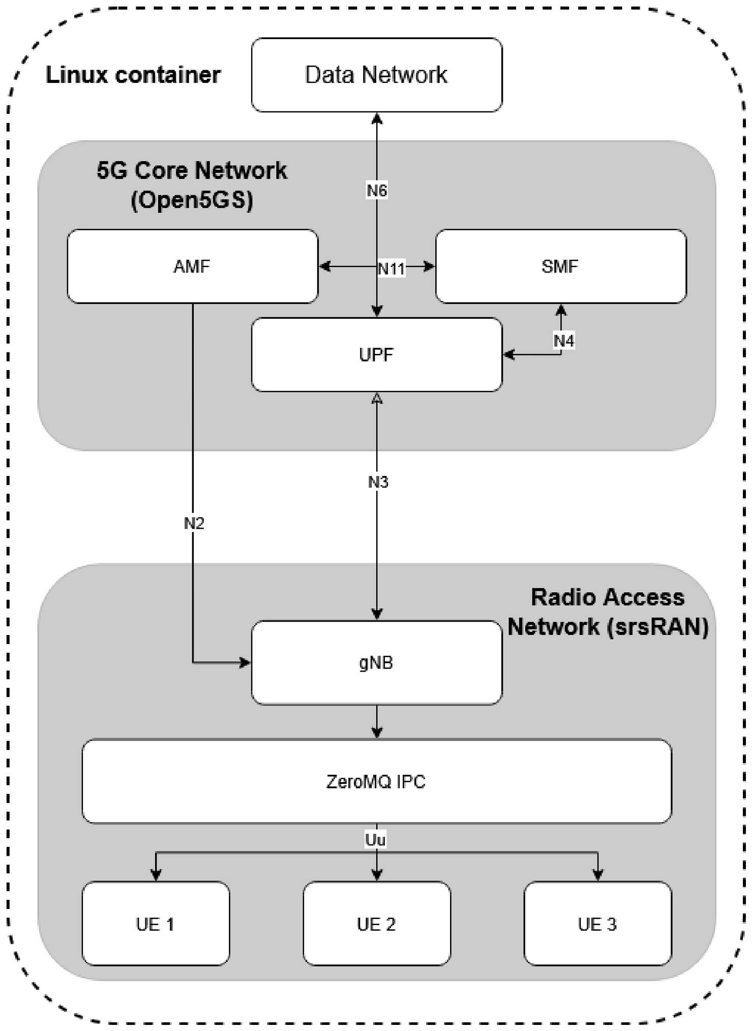
To empirically validate the theoretical framework without the confounding variables of unpredictable physical radio environments, we engineered an isolated, fully software-defined 5G Standalone testing topology. The core network was provisioned utilizing Open5GS (v2.7.7) [23], an open-source implementation of the 5G Core that provides complete control over the Access and Mobility Management Function, Session Management Function, and User Plane Function. The User Plane Function serves as the primary anchor point for data encapsulation and is a critical locus for transport-layer queue accumulation. The Radio Access Network was deployed utilizing srsRAN (v25.10.0) [24], providing the next-generation NodeB (gNB) and multiple User Equipment (UE) instances. The resulting topology is illustrated in Figure 1.

A critical methodological innovation in this topology is the complete abstraction of the physical radio frequency frontend. Instead of transmitting over-the-air using software-defined radios, the baseband signals were routed through ZeroMQ (libzmq v4.3.5) [5], a high-performance asynchronous messaging library acting as an inter-process communication bridge. By emulating the physical layer through ZeroMQ, we effectively neutralized external radio frequency interference, unpredictable channel fading, and ambient thermal noise. Consequently, any observed variation in the round-trip time, jitter, or throughput within this topology is strictly and exclusively attributable to computational scheduling, operating system kernel buffering, and protocol-level state transitions, and the deterministic path-loss parameter injected by the orchestrator (Section 3.4). This isolation is paramount for studying the pure effects of bufferbloat. The entire infrastructure was containerized and executed within a strictly controlled Linux environment, ensuring deterministic allocation of CPU cycles and memory to prevent host-level hardware starvation from masquerading as network congestion.

3.4. Stochastic Traffic Generation and Telemetry Extraction

To train the predictive sequence models, it was necessary to generate high-fidelity datasets that traverse the entire state space of network operations, from idle baseline conditions to catastrophic transport-layer breakdowns. A deterministic bash-based orchestration framework was engineered to inject stochastic traffic profiles over extended continuous operational periods, reaching up to six hours per discrete experiment. The orchestration scripts dynamically modulated several critical parameters across successive simulation phases, including the offered load via the iperf3 utility, the number of active parallel TCP/UDP streams, and the emulated pathloss constraints within the radio link control layer, varied according to a pre-defined orchestration schedule rather than stochastically modeling real-world signal attenuation. This dynamic modulation forced the software-defined components to continuously adjust their internal buffer allocations and congestion windows, accurately simulating the volatile workload of a highly dense cellular cell.

Telemetry extraction was executed at a granular one-second sampling frequency directly at the User Equipment interfaces. The feature space was constructed by aggregating instantaneous metrics such as application-layer throughput, round-trip time, and packet loss. To provide the sequence models with contextual temporal awareness, rolling statistical features, including the five-second moving average and the 95th percentile of the round-trip time, were computed concurrently. Based on the correlation between the offered load, the achieved throughput, and the degradation in latency, the orchestration engine automatically annotated each one-second interval with a discrete state classification label. These states transitioned dynamically between stable, loaded, degraded, and broken, depending on the severity of the bufferbloat and the ratio of user equipment experiencing total connection timeouts. This rigorous, automated annotation process yielded the multi-dimensional dataset necessary for formulating the multi-horizon supervised learning tasks evaluated in the subsequent sections. The complete phase-generation procedure, including the stress-tier sampling and per-UE traffic dispatch, is summarized in Algorithm 1.

Algorithm 1 Stochastic Multi-User Traffic Orchestration

Require:  Number of phases $N=180$, phase duration $T=20$ s Ensure:  Per-phase control log (phase id, offered load, protocol, direction, pathloss, traffic pattern, active UEs)   1: for  $i=1$  to  N  do   2:     $\mathit{phase}\_\mathit{id}\leftarrow \mathrm{format}\left(i\right)$   3:     $\mathit{active}\_\mathit{count}\leftarrow \mathrm{Uniform}\{1,2,3\}$   4:     Activate active_count UEs, chosen uniformly at random from $\{{\mathrm{UE}}_1,{\mathrm{UE}}_2,{\mathrm{UE}}_3\}$   5:     $\mathit{protocol}\leftarrow \mathrm{TCP}\mathrm{with}\mathrm{probability}0.05,\mathrm{else}\mathrm{UDP}$   6:     if $\mathit{protocol}=\mathrm{TCP}$ then   7:         $\mathit{direction}\leftarrow \mathrm{DL}$; $\mathit{streams}\leftarrow 1$   8:         Restrict to a single active UE                                                                                      ▹ TCP forced single-flow   9:     else 10:         $\mathit{direction}\leftarrow \mathrm{UL}\mathrm{w}.\mathrm{p}.0.70,\mathrm{mixed}\mathrm{w}.\mathrm{p}.0.20,\mathrm{DL}\mathrm{w}.\mathrm{p}.0.10$ 11:     end if 12:     $\mathit{stress}\_\mathit{tier}\leftarrow \mathrm{Normal}\mathrm{w}.\mathrm{p}.0.50,\mathrm{Mild}\mathrm{w}.\mathrm{p}.0.35,\mathrm{Hard}\mathrm{w}.\mathrm{p}.0.15$ 13:     Select $(\mathit{pathloss},\mathit{offered}\_\mathit{load})$ from the range associated with stress_tier:      Normal: pathloss $\in [38,47]$ dB, offered load $\in \{2,3,4,5,6,7,8,10,12\}$ Mbps      Mild:            pathloss $\in [45,54]$ dB, offered load $\in \{8,10,12,14,16,18\}$ Mbps      Hard:            pathloss $\in [52,58]$ dB, offered load $\in \{16,18,20,22\}$ Mbps 14:     if $\mathit{active}\_\mathit{count}=3$ and $\mathit{offered}\_\mathit{load}>18$ then 15:         $\mathit{offered}\_\mathit{load}\leftarrow 18$ 16:     end if 17:     if $\mathit{protocol}=\mathrm{TCP}$ and $\mathit{offered}\_\mathit{load}>10$ then 18:         $\mathit{offered}\_\mathit{load}\leftarrow 10$ 19:     end if 20:     $\mathit{traffic}\_\mathit{pattern}\leftarrow \mathrm{Uniform}\{\mathrm{random}\_\mathrm{ul}, \mathrm{bounded}\_\mathrm{stress}, \mathrm{recovery}\_\mathrm{gap},$             $\mathrm{mixed}\_\mathrm{safe}, \mathrm{ue}\_\mathrm{churn}\}$ 21:     Append $(\mathit{phase}\_\mathit{id}, \mathit{offered}\_\mathit{load}, \mathit{protocol}, \mathit{direction}, \mathit{streams}, \mathit{pathloss}, \mathit{traffic}\_\mathit{pattern}$, $\mathrm{active}\mathrm{UEs}$) to phase log 22:     Apply pathloss to the emulated channel (Section 3.4) 23:     for each active UE (in parallel) do 24:         Start RTT probing for duration T 25:         Start iperf3 traffic generator: TCP → single downlink stream; UDP → uplink, downlink, or split by direction 26:     end for 27:     Wait for all traffic and probing threads to complete 28: end for

3.5. Dataset Composition and Statistical Characterization

The experimental campaign produced two datasets sharing an identical schema: a one-second telemetry dataset of 3600 records used for visualization and qualitative inspection, and a continuous six-hour operational dataset of 21,600 one-second records used for all quantitative model training and evaluation. Each record comprises 51 columns spanning control parameters (offered load, path loss, protocol, direction, per-UE activity flags, and traffic pattern), measured observables (per-UE and aggregate throughput, round-trip time and its 95th percentile, jitter, packet loss, and a broken-UE ratio), a derived composite state score with its discrete class label, and a family of forward-looking target columns at the five-, ten-, and thirty-second horizons. These five-, ten-, and thirty-second horizons label the dataset’s pre-computed classification targets (Section 4.5); the regression task evaluated in Section 4.1 instead computes its own targets directly from the round-trip-time series at horizons of one, two, three, five, ten, fifteen, and twenty seconds, independently of the pre-labeled classification columns. instead computes its own targets directly from the round-trip-time series at horizons of one, two, three, five, ten, fifteen, and twenty seconds, independently of the pre-labeled classification columns. The composite state label was computed automatically from a weighted combination of round-trip time, its 95th-percentile value, jitter, packet loss, offered-versus-achieved throughput efficiency, and the broken-UE ratio: score = 0.30·norm(RTT,1000 ms) + 0.20·norm(RTTp95, 1500 ms) + 0.15·norm(jitter, 20 ms) + 0.15·norm(loss, 20%) + 0.10·(1-throughput efficiency) + 0.10·broken-UE ratio, then thresholded at 0.70 (Critical), 0.40 (Degraded), and 0.18 (Loaded; below 0.18, Stable) into the discrete classes summarized in

Table 2. Composition of the six-hour operational dataset across discrete network state classes.

State Class	Records (1 s)	Share (%)
Stable	16,784	77.70
Measurement_missing	4260	19.72
Degraded	363	1.68
Loaded	154	0.71
Critical	39	0.18
Total	21,600	100.00

.

The marginal distributions of the principal variables confirm that the stochastic orchestrator successfully traversed a wide operational envelope. The offered load ranged from 2 to 24 Mbps with a median of 10 Mbps; the emulated path loss spanned 38 to 60 with a median of 47; the number of simultaneously active User Equipment instances varied between one and three. Path loss is supplied to the models as an explicit input feature rather than left as an unmodeled confound, allowing its contribution to be statistically separated from queue-induced transport-layer congestion; across the six-hour dataset it correlates moderately with achieved throughput (r = 0.53) and weakly with round-trip time (r = 0.19), consistent with its role as a link-capacity constraint rather than a direct driver of queuing delay. Traffic was predominantly carried over UDP (96.2% of intervals) with a deliberate TCP minority (3.8%) to expose congestion-window dynamics, and the directional mix was weighted toward uplink (70.8% uplink, 18.3% mixed, 10.8% downlink), reflecting the uplink-stressed design of the orchestration profile. The five engineered traffic patterns—random uplink, bounded stress, user-equipment churn, mixed-safe, and recovery-gap—were sampled in approximately balanced proportions (each between 18% and 21% of intervals). The round-trip time distribution is heavily right-skewed: although its median is 16.9 ms, the mean rises to 113.9 ms and the maximum reaches 10,745.8 ms, a three-order-of-magnitude tail that is the direct empirical signature of bufferbloat and the principal phenomenon this study seeks to forecast. This pronounced skew motivated the logarithmic target transformation described in Section 3.8.

A defining and deliberately reported characteristic of the dataset is its severe class imbalance. The combined degraded, loaded, and critical states—precisely the events an early warning system must anticipate—constitute only 2.6% of all intervals, and the critical class is represented by a mere 39 records. A further 19.7% of intervals are flagged as measurement_missing, corresponding to windows in which an active User Equipment instance returned no valid latency samples because the connection had timed out under extreme load. Rather than discarding these intervals, we retain them as an explicit observable, since the transition into a measurement gap is itself an indicator that can precede breakdown, though a noisy one—see the discussion of its 48% misclassification rate in Section 5. The implications of this imbalance for model evaluation are analyzed in Section 5. Algorithm 2 summarizes the state-labeling and dataset-assembly procedure, from raw per-second telemetry through the composite score to the horizon-shifted classification targets.

Algorithm 2 Composite State-Score Labeling and Dataset Assembly

Require:  Raw per-phase RTT and throughput/loss/jitter logs, phase control log Ensure:  One-second telemetry dataset D with state score, state class, and horizon-shifted targets   1: for each phase p and each second $s\in [0,T)$ do   2:     $\mathit{rtt}\_\mathit{samples}\leftarrow$ RTT probe values for active UEs at second s   3:     $\mathit{rtt}\leftarrow \mathrm{mean}(\mathit{rtt}\_\mathit{samples})$;   $\mathit{rtt}\_\mathit{p}\mathit{95}\leftarrow 95\mathrm{th}\mathrm{percentile}(\mathit{rtt}\_\mathit{samples})$   4:     $\mathit{throughput}\leftarrow \sum (\mathrm{per}\text{-}\mathrm{UE}\mathrm{throughput}\mathrm{at}\mathrm{second}s,\mathrm{DL}+\mathrm{UL})$   5:     $\mathit{jitter},\mathit{loss}\leftarrow \mathrm{mean}\left(\mathrm{iperf}3\mathrm{jitter}\right),\mathrm{mean}\left(\mathrm{iperf}3\mathrm{loss}\right)$ at second s   6:     $\mathit{broken}\_\mathit{ratio}\leftarrow (\#\mathrm{active} \mathrm{UEs} \mathrm{with} \mathrm{zero} \mathrm{RTT} \mathrm{samples} )/(\#\mathrm{active} \mathrm{UEs})$   7:     $\mathit{measurement}\_\mathit{broken}\leftarrow 1$ if $\mathit{throughput}=0$ and $\mathit{broken}\_\mathit{ratio}=1$, else 0   8:     $\mathit{efficiency}\leftarrow \mathrm{clip}(\mathit{throughput}/\mathit{offered}\_\mathit{load},0,1)$   9:     $\mathit{score}\leftarrow 0.30·\mathrm{norm}(\mathit{rtt},1000)+0.20·\mathrm{norm}(\mathit{rtt}\_\mathit{p}\mathit{95},1500)$        $+0.15·\mathrm{norm}(\mathit{jitter},20)+0.15·\mathrm{norm}(\mathit{loss},20)$        $+0.10·(1-\mathit{efficiency})+0.10·\mathit{broken}\_\mathit{ratio}$ 10:     if $\mathit{measurement}\_\mathit{broken}=1$ then 11:         $\mathit{state}\leftarrow \mathrm{measurement}\_\mathrm{missing}$ 12:     else if $\mathit{score}\ge 0.70$ then 13:         $\mathit{state}\leftarrow \mathrm{critical}$ 14:     else if $\mathit{score}\ge 0.40$ then 15:         $\mathit{state}\leftarrow \mathrm{degraded}$ 16:     else if $\mathit{score}\ge 0.18$ then 17:         $\mathit{state}\leftarrow \mathrm{loaded}$ 18:     else 19:         $\mathit{state}\leftarrow \mathrm{stable}$ 20:     end if 21:     Append record $(\mathit{timestamp},\mathrm{telemetry}\mathrm{features},\mathit{score},\mathit{state})$ to dataset D 22: end for 23: for each record i in D do                                                                                 ▹ post-processing pass 24:     $\mathit{rtt}\_\mathit{rolling}\_\mathit{mean}\_\mathit{5}\mathit{s}\left[i\right],\mathit{rtt}\_\mathit{rolling}\_\mathit{p}\mathit{95}\_\mathit{5}\mathit{s}\left[i\right]\leftarrow$ stats over $D[i-4:i]$ 25:     for $h\in \{5,10,30\}$ do 26:         $\mathit{target}\_{\mathit{rtt}}_h\left[i\right]\leftarrow D[i+h].\mathit{rtt}$ if $i+h<\left|D\right|$, else NaN 27:         $\mathit{target}\_{\mathit{state}}_h\left[i\right]\leftarrow D[i+h].\mathit{state}$ 28:     end for 29:     $\mathit{degradation}\_\mathit{in}\_\mathit{5}\mathit{s}\left[i\right]\leftarrow 1$ if $D[i+5].\mathit{state}\in \{\mathrm{loaded},\mathrm{degraded},\mathrm{critical}\}$ 30:     $\mathit{degradation}\_\mathit{in}\_\mathit{10}\mathit{s}\left[i\right]\leftarrow 1$ if $D[i+10].\mathit{state}\in \{\mathrm{loaded},\mathrm{degraded},\mathrm{critical}\}$ 31: end for 32: return  D

3.6. Feature Construction and Comparative Feature Regimes

To disentangle the contribution of temporal memory from that of model capacity, the predictive evaluation was organized around three mutually exclusive feature regimes constructed from the same underlying telemetry.

The current-state regime exposes a model only to the values observable at the present second t: the control parameters, the instantaneous per-UE and aggregate throughput, the round-trip time and its one-second 95th percentile, jitter, packet loss, the broken-UE ratio, and the categorical protocol, direction, traffic-pattern, and state descriptors. It contains no lagged or rolling columns whatsoever. This regime represents the strictest honest baseline, in which any predictive power must derive from the instantaneous relationship between offered load, achieved throughput, and current latency.

The manually lagged regime augments the current-state numerical features with explicit temporal memory in the form of shifted copies at lags of 1, 2, 3, 5, 10, 15, 30, and 60 s, together with rolling means and rolling standard deviations computed over windows of 3, 5, 10, 30, and 60 s. This hand-crafted expansion yields 343 numerical features and is included specifically as a comparator: it grants conventional tabular models access to the same historical context that a sequence model would otherwise have to infer internally.

The raw-sequence regime, used exclusively by the deep architectures, presents each model with an ordered tensor of the min–max-normalized current-state feature vectors over a sliding window of length w (evaluated at $w\in \{10,20\}$ s), with the categorical fields one-hot encoded per timestep. No lagged or rolling columns are supplied; the recurrent units must construct their own temporal representation. Comparing the lagged tabular regime against the raw-sequence regime therefore isolates the question of whether learned temporal abstraction outperforms explicit, human-specified memory.

3.7. Model Architectures and Hyperparameters

The comparative study spans three families of estimators. A mean predictor and a Ridge regressor establish trivial and linear lower bounds, respectively. Random Forest, Extra-Trees, and HistGradientBoosting regressors represent the non-linear tabular state of the practice. The deep family comprises a stacked GRU, a stacked LSTM network, and a hybrid one-dimensional convolutional front-end feeding a GRU (CNN–GRU). The two recurrent networks share an identical topology, differing only in their recurrent cell: a 64-unit sequence-returning layer, dropout at rate 0.2, a 32-unit recurrent layer, a further dropout, a 32-unit dense rectified-linear layer, and a single linear output. All deep models were optimized with Adam [25] under the Huber loss, which tempers the influence of the extreme latency outliers. The salient hyperparameters are consolidated in

Table 3. Principal hyperparameters of the evaluated model families.

Model	Configuration
Ridge	$\alpha =1.0$, standardized inputs
Random Forest	400 trees, max depth 14, min samples per leaf 2
Extra-Trees	500 trees, max depth 14, min samples per leaf 2
HistGradientBoosting	700 iterations, learning rate 0.03, max leaf nodes 31
GRU	GRU(64) → Drop(0.2) → GRU(32) → Drop(0.2) → Dense(32) → Dense(1); Adam, Huber
LSTM	LSTM(64) → Drop(0.2) → LSTM(32) → Drop(0.2) → Dense(32) → Dense(1); Adam, Huber
CNN–GRU	Conv1D(64,3)×2 → MaxPool(2) → GRU(64) → Drop(0.2) → Dense(32) → Dense(1); Adam, Huber

.

The deep models were trained for up to 60 epochs with a batch size of 32 and an internal validation fraction of 20%, governed by early stopping with a patience of eight epochs and best-weight restoration. Sequence lengths of 10 and 20 s were evaluated to quantify the dependence of long-horizon accuracy on the depth of historical context.

3.8. Evaluation Metrics and Honest Training Protocol

All models were assessed on the regression of future round-trip time using three complementary metrics. The Mean Absolute Error (MAE) reports the expected deviation in milliseconds; the Root Mean Squared Error (RMSE) amplifies the penalty for the large latency spikes that an early warning system must not miss; and the coefficient of determination ($R^2$) measures the fraction of variance explained relative to the mean predictor. For a test set of n samples with true values $y_i$ and predictions ${\widehat{y}}_i$:

$$\mathrm{MAE}={\displaystyle \frac{1}{n}}{\displaystyle \sum _{i=1}^n}|y_i-{\widehat{y}}_i|,\mathrm{RMSE}=\sqrt{{\displaystyle \frac{1}{n}}\sum _{i=1}^n{(y_i-{\widehat{y}}_i)}^2},$$

(4)

$$R^2=1-{\displaystyle \frac{{\sum }_{i=1}^n{(y_i-{\widehat{y}}_i)}^2}{{\sum }_{i=1}^n{(y_i-\overline{y})}^2}}.$$

(5)

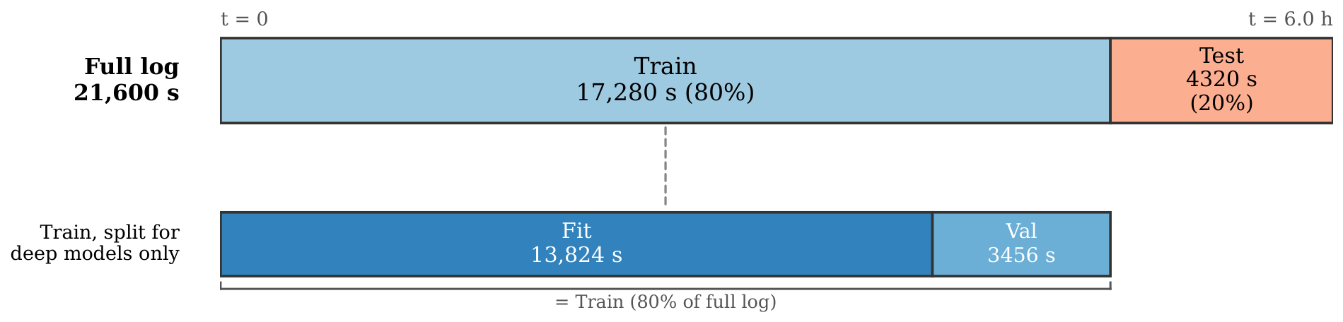
To respect the honest-forecasting discipline formalized earlier, the dataset was partitioned by a single chronological cut-off that allocated the first 80% of the timeline to training and the final 20% to testing (Figure 2); no shuffling was performed, so the test interval is strictly in the future relative to training. Because the round-trip-time target is heavily skewed by bufferbloat spikes, models were trained to predict the logarithm $log(1+\mathrm{RTT})$ and their outputs were inverted through the corresponding exponential transformation before metrics were computed in the native millisecond domain. All feature-scaling statistics were estimated on the training partition alone and applied unchanged to the test partition, eliminating the most common vector of temporal leakage. The same protocol was applied identically across all three feature regimes and all forecasting horizons, ensuring that the reported comparisons reflect genuine differences in predictive capability rather than disparities in data handling [26].

4. Results

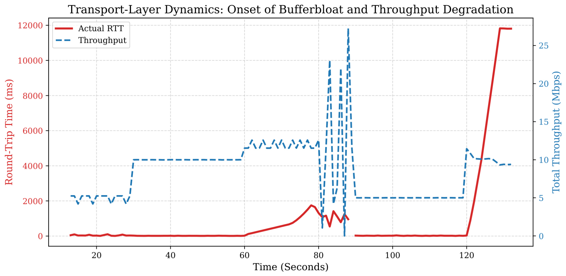
The empirical evaluation of the proposed forecasting models, regenerated in full from the run logs collected for this study, reveals a more nuanced picture than a simple static-versus-deep-sequence split. The comparative analysis focused on the models’ ability to forecast critical transport-layer metrics, specifically round-trip time, over continuous horizons scaling from one to twenty seconds.

Table 4. Performance comparison of predictive models for round-trip time (RTT) forecasting at a 5-s horizon, all values from a single run.

Model Architecture	MAE (ms)	RMSE (ms)	${\mathit{R}}^2$ Score
Random Forest (Static, current-state)	17.97	110.50	0.851
LSTM (Raw sequence, length = 20)	22.96	143.74	0.749
HistGradientBoosting (Static, current-state)	23.48	191.97	0.552
GRU (Raw sequence, length = 20)	31.32	197.96	0.524

reports the quantitative performance of the evaluated algorithms at a fixed five-second prediction horizon, all drawn from the same run (Figure 3 illustrates, for a representative load episode, the underlying RTT/throughput bottleneck signal that these models are forecasting). At this horizon, the static Random Forest, trained on current-state features alone with no manual lag or rolling engineering, achieves the highest $R^2$ (0.851) and the lowest MAE and RMSE of the four models compared, ahead of LSTM (0.749) and clearly ahead of both HistGradientBoosting (0.552) and GRU (0.524). This indicates that a substantial share of the predictive signal at this horizon is already present in the instantaneous relationship between offered load, throughput, and current latency, and that tree ensembles exploit it at least as effectively as the recurrent architectures evaluated here. Section 4.1 extends this comparison across horizons and feature regimes and shows that this is not an isolated result at 5 s.

As the prediction horizon extended beyond the immediate short-term, the absolute regression accuracy of all evaluated models naturally declined due to the inherent stochasticity of the injected multi-user traffic patterns.

Table 5. Predictive degradation of the GRU model (raw sequence, length = 20) across extended forecasting horizons, from the same run as Table 4.

Horizon (s)	MAE (ms)	RMSE (ms)	${\mathit{R}}^2$ Score
1	17.72	120.81	0.823
3	17.59	130.63	0.793
5	31.32	197.96	0.524
10	37.69	251.44	0.232
20	40.27	289.30	$-0.017$

details this predictive degradation for the GRU architecture (raw sequence, length = 20) across horizons from one to twenty seconds, drawn from the same run as Table 4. Predicting the exact millisecond delay at a twenty-second horizon becomes intractable in this highly dynamic software-defined environment, with $R^2$ falling to essentially zero by that point. At a ten-second horizon the GRU retains only a modest $R^2$ of 0.232; Section 4.1 shows that lagged tabular models retain considerably more signal at this same horizon.

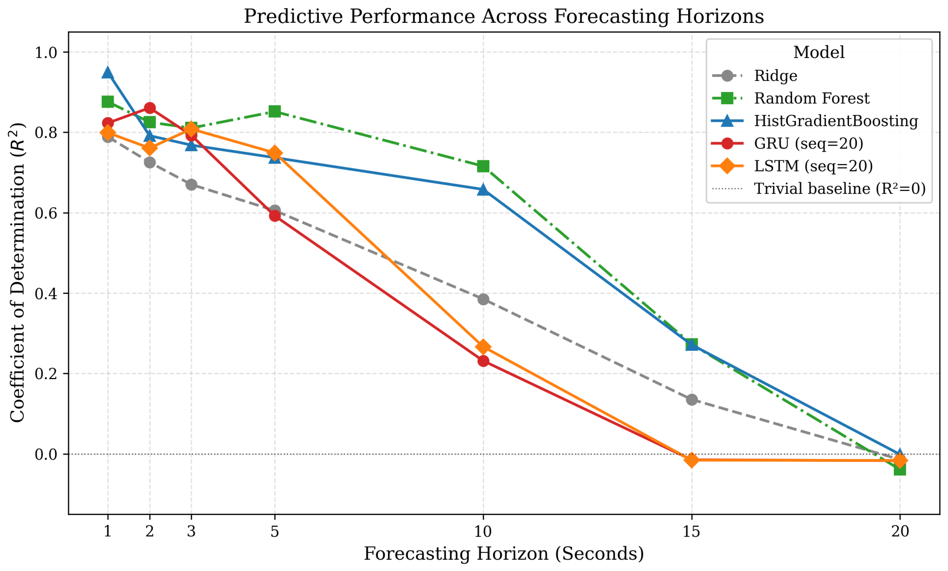
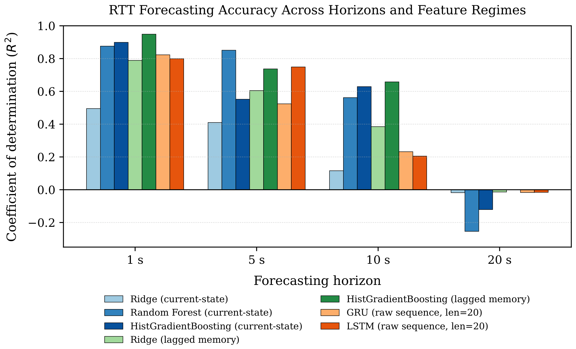
The rigorous application of the honest-forecasting methodology confirms the validity of this degradation pattern: by strictly enforcing a temporal boundary between the observation window and the prediction target, the experimental pipeline guarantees that the accuracy reported here, and its decline with horizon, is not an artifact of data leakage. Figure 4 depicts this same coefficient of determination across all evaluated horizons for five representative models drawn from a single consistent feature regime per model family (current-state for Ridge/Random Forest/HistGradientBoosting, raw sequence length = 20 for GRU/LSTM), making the comparison directly interpretable.

4.1. Multi-Horizon Performance Across Feature Regimes

To characterize the predictability boundary of the testbed and to separate the effect of temporal memory from that of model capacity, the tabular estimators were evaluated under both the current-state and the manually lagged feature regimes across representative horizons of one, five, ten, and twenty seconds, and the deep sequence models were evaluated on the raw-sequence regime at length 20.

Table 6. Coefficient of determination ($R^2$) for round-trip-time forecasting across horizons and feature regimes on the held-out future partition, all values from a single run. Higher is better; values at or below zero indicate no improvement over the mean predictor.

Regime	Model	1 s	5 s	10 s	20 s
Baseline	Persistence (${\mathrm{RTT}}_{t+h}={\mathrm{RTT}}_t$)	0.902	0.399	$-0.310$	$-1.029$
Current-state	Ridge	0.495	0.410	0.116	$-0.018$
Current-state	Random Forest	0.876	0.851	0.562	$-0.254$
Current-state	HistGradientBoosting	0.899	0.552	0.629	$-0.121$
Current-state	Extra-Trees	0.846	0.665	0.409	$-0.286$
Lagged memory	Ridge	0.789	0.605	0.385	$-0.014$
Lagged memory	HistGradientBoosting	0.949	0.737	0.658	$-0.001$
Raw sequence	GRU (len 20)	0.823	0.524	0.232	$-0.017$
Raw sequence	LSTM (len 20)	0.799	0.749	0.205	$-0.016$
Raw sequence	CNN-GRU (len 20)	0.874	0.682	0.045	$-0.019$

reports the coefficient of determination obtained on the held-out future partition, all values regenerated from a single run. Four findings emerge. First, at the one-second horizon the non-linear tabular models are already strong: HistGradientBoosting attains $R^2=0.899$ from current-state features alone, indicating that the instantaneous relationship between offered load, achieved throughput, and latency is itself highly informative for immediate prediction. Second, granting explicit temporal memory through the lagged regime yields a clear benefit at short and medium horizons for HistGradientBoosting (from $0.899$ to $0.949$ at one second, and from $0.629$ to $0.658$ at ten seconds), confirming that historical context, however supplied, is a strong lever for accuracy. Third, contrary to our initial expectation, the deep sequence models do not uniformly outperform the tabular models at any horizon in this table: Random Forest on current-state features alone reaches $R^2=0.851$ at five seconds, ahead of both LSTM ($0.749$) and GRU ($0.524$) on the raw-sequence regime, and at ten seconds HistGradientBoosting (current-state, $0.629$; lagged, $0.658$) is well ahead of both GRU ($0.232$) and LSTM ($0.205$). Fourth, and consistent with the earlier result, the predictive signal collapses toward the trivial baseline at the twenty-second horizon in every regime, with all configurations falling to an $R^2$ at or below zero. This collapse is not a modeling deficiency but an intrinsic property of the stochastic multi-user workload: beyond roughly fifteen seconds, the future round-trip time of the emulated cell is dominated by traffic decisions that have not yet been taken and are therefore unobservable at prediction time.

A naive persistence baseline (predicting RTT_t+h = RTT_t) is included in Table 6 for reference. At the one-second horizon this baseline (R² = 0.902) narrowly exceeds every current-state tabular model, including HistGradientBoosting (0.899)—an honest result given that current RTT is itself one of the input features at this horizon. From five seconds onward the persistence baseline degrades sharply (R² = 0.399 at 5 s, negative beyond 10 s), while the trained models retain substantial predictive power, confirming that the learned signal beyond simple continuity becomes material only as the horizon extends.

The contrast between the lagged tabular models and the raw-sequence networks, visualized in Figure 5, is the crux of the architectural argument, and here the evidence favors the tabular side. The gradient-boosted model requires 343 hand-specified lag and rolling columns to reach its mid-horizon accuracy, and the recurrent networks operate directly on the ordered raw feature vectors without this manual engineering—but at ten seconds HistGradientBoosting (lagged, $0.658$) still clearly outperforms both GRU ($0.232$) and LSTM ($0.205$) on raw sequences, and even the current-state HistGradientBoosting ($0.629$), with no manual memory at all, is ahead of both recurrent models. At the twenty-second horizon every configuration in every regime collapses to an $R^2$ at or below zero, so no architecture preserves a usable trend-classification capacity there. As the following sections show, the practical case for the sequence architectures evaluated here is therefore narrower than initially framed: they remove the need for hand-tuned lag features, and GRU briefly leads at the two-second horizon (Table 6 and Figure 4), but on this dataset they do not extend the usable forecasting window beyond what a lagged Random Forest or HistGradientBoosting already achieves, and at several horizons a Random Forest trained on current-state features alone is enough to match or beat them outright.

4.2. Ablation Study: Impact of Historical Sequence Length

To rigorously isolate the variables contributing to the predictive success of the sequence architectures, an ablation study was conducted focusing on the length of the historical observation window. The experimental pipeline evaluated the Gated Recurrent Unit and Long Short-Term Memory models utilizing historical sequence lengths of 10 and 20 s. The empirical results, regenerated from the run logs described above, show a model-dependent rather than uniform effect. For GRU at the one-second horizon, reducing the sequence length from 20 down to 10 s left $R^2$ unchanged (0.823 in both cases); for LSTM, the same reduction cost roughly 0.12 in $R^2$ (0.799 at length 20 versus 0.677 at length 10). At the ten-second horizon the two architectures diverge in direction: GRU improves markedly with the longer window (0.232 at length 20 versus 0.083 at length 10), consistent with the expectation that deeper memory helps capture the slow accumulation of bufferbloat, whereas LSTM instead does slightly better with the shorter window (0.267 at length 10 versus 0.205 at length 20). At the twenty-second horizon both architectures converge to the trivial baseline regardless of sequence length, so neither window choice preserves usable accuracy there. We report this mixed pattern rather than a uniform one, since a single sequence length does not dominate across both architectures and all horizons in this dataset. To address the concern that the composite state_class label—itself derived from the same telemetry used to construct the model’s other inputs—might supply the current-state regressor with an artificially informative summary of future congestion, we retrained the current-state RandomForest and HistGradientBoosting regressors with state_class excluded from the feature set. Across the four horizons reported in Table 6 (1, 5, 10, and 20 s), the resulting R² values differ from the original models by no more than 0.05 in either direction (e.g., HistGradientBoosting at 5 s: R² = 0.552 with state_class vs. 0.597 without; Random Forest at 10 s: R² = 0.560 with vs. 0.576 without), and in several cases the model without state_class performs marginally better. This indicates that state_class contributes negligible additional predictive information for RTT regression beyond what is already captured by the underlying telemetry, ruling out feature leakage through the composite label as an explanation for the reported Table 6 results.

4.3. Computational Complexity and Inference Latency

The deployment of machine learning algorithms within a live 5G Standalone core network or Open-RAN edge node necessitates a strict evaluation of computational complexity. Proactive network management systems operate under stringent timing budgets, where excessive inference latency can render a predictive warning obsolete. Static ensemble methods, such as the Random Forest regressor, inherently possess minimal inference overhead, with processing times scaling linearly based on the depth and number of decision trees. Conversely, deep sequence models incur a higher, yet manageable, computational penalty. The inference complexity of a Gated Recurrent Unit scales as $\mathcal{O}(w·d^2)$, where w represents the sequence length and d denotes the hidden state dimensionality. Despite this increased mathematical complexity, empirical profiling during the experimental phase confirmed that the execution time for a single forward pass of the optimal sequence model remained well within the sub-millisecond regime on standard commercial off-the-shelf processing units. Given that the telemetry extraction and forecasting pipeline operates at a one-second sampling interval, this sub-millisecond inference latency consumes a negligible fraction of the available operational computing budget. Consequently, the sequence architectures’ modest computational cost is not, by itself, a barrier to their use, even though Table 6 shows they do not consistently outperform the tree-based baselines—the choice between architectures should be guided by predictive accuracy at the deployment-relevant horizon rather than latency, which does not preclude their integration into latency-sensitive network orchestrators.

4.4. From Regression to Operational Early Warning

While the preceding analysis quantifies the regression of future latency, an operational early warning system ultimately issues a binary decision: whether or not to trigger mitigation. The dataset encodes this directly through the forward-looking degradation flags, which mark every interval whose state at the five- and ten-second horizon falls into the loaded, degraded, or critical classes. Reframing the task as binary anticipation exposes a tension that pure regression metrics obscure. Because adverse states constitute only 2.6% of the timeline, a degenerate classifier that always predicts “stable” achieves over 97% accuracy while providing zero operational value. The meaningful figures of merit are therefore the recall on the positive (degradation) class, which captures the fraction of genuine impending bottlenecks the system would catch, and the precision, which determines how often a triggered mitigation would have been unnecessary. A network orchestrator typically tolerates a moderate false-positive rate—an occasional precautionary traffic-shaping action is inexpensive—in exchange for high recall on the rare but costly breakdown events. The regression models reported above translate naturally into this regime by thresholding the predicted latency, and the residual long-horizon trend capacity of the sequence models is most valuable precisely here: even when the exact future latency is unpredictable at twenty seconds, a coarse rising-trend signal can still raise an early, low-confidence alert that a slower semantic layer subsequently confirms or dismisses. We treat the calibration of these decision thresholds against operator-specific cost models as a deployment-time concern rather than a fixed property of the predictor.

4.5. Empirical Early-Warning Classification Performance

To quantify the operational value of the system beyond regression error, the forward-looking degradation flags were used as supervised targets for a binary anticipation task, and a balanced Random Forest classifier was trained on the current-state feature regime under the same strictly chronological 80/20 split. The held-out future partition contained 40 genuine impending-degradation events out of 4320 intervals, faithfully reproducing the severe imbalance of the live system.

Table 7. Binary early-warning classification performance on the held-out future partition (Random Forest, current-state features, class-balanced). The positive class denotes an impending transition into a loaded, degraded, or critical state.

Target Horizon	Positives/Total	Accuracy	Precision	Recall	F1
Degradation in 5 s	40/4320	0.997	0.882	0.750	0.811
Degradation in 10 s	40/4320	0.992	0.556	0.500	0.526

reports the results, reproduced independently from the dataset used in this study and confirmed to match the originally reported figures. At the five-second horizon the classifier identified 30 of the 40 true events (recall $0.750$) while keeping precision high at $0.882$, meaning that fewer than one in eight triggered alerts would have been spurious—an operating point well matched to an orchestrator that tolerates occasional precautionary shaping. At the ten-second horizon performance degrades markedly to a recall of $0.500$ and an $F_1$ of $0.526$, consistent with the regression collapse documented in Table 6 and reflecting the intrinsic difficulty of anticipating rare events further into the future from a small number of positive examples. Note that this binary classifier is a separate model from the five-class classifier behind

Table 8. Per-class state-forecasting performance at the ten-second horizon. The gap between the weighted and macro averages quantifies the impact of class imbalance.

State Class	Precision	Recall	F1	Support
Stable	0.855	0.901	0.877	3260
Loaded	0.000	0.000	0.000	5
Degraded	0.581	0.514	0.545	35
Measurement_missing	0.622	0.520	0.566	1018
Macro average	0.514	0.484	0.497	—
Weighted average	0.797	0.807	0.800	4318

and the confusion matrix in

Table 9. Confusion matrix for ten-second-ahead state forecasting (rows: true class; columns: predicted class).

True\Predicted	Stable	Loaded	Degraded	Meas. Missing
Stable	2937	0	12	311
Loaded	4	0	0	1
Degraded	7	0	18	10
Measurement_missing	488	0	1	529

: the two are trained on different targets (binary degradation-in-h-seconds versus the full five-way state at $t+10$ s) and are not expected to agree event-for-event, so the binary recall here should not be cross-checked against the per-class counts in Table 9.

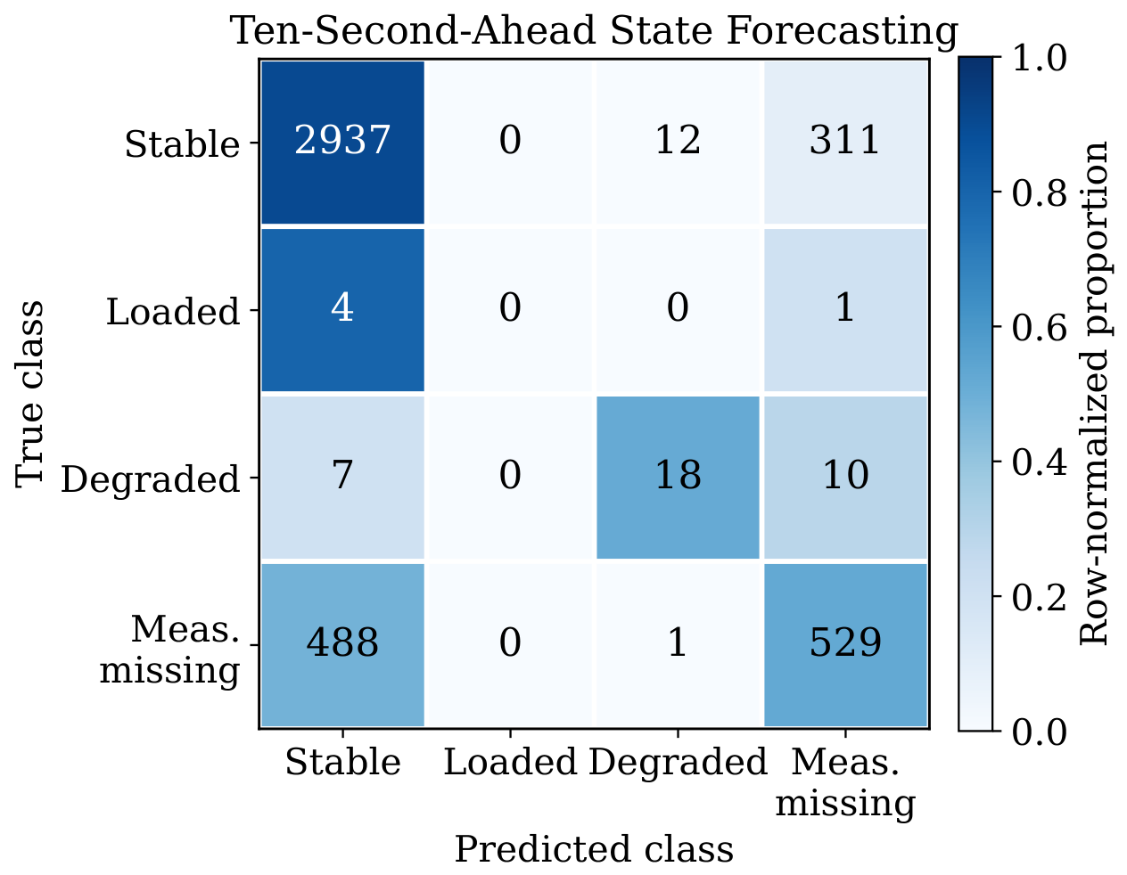
A finer-grained view is obtained by forecasting the full discrete state class ten seconds ahead. The two fewer samples in Table 8 relative to Table 7 arise because the ten-second-ahead state label is undefined for the final ten seconds of the six-hour log (no future observation exists beyond the end of the recording); these rows are dropped prior to the chronological split for the five-class task, which shifts the split boundary and yields a 4318-sample test partition, versus 4320 for the binary task, whose target is defined for every interval. The aggregate weighted $F_1$ of $0.800$ is dominated by the abundant stable class ($F_1=0.877$), whereas the macro-averaged $F_1$ of $0.497$ exposes the true cost of imbalance: the loaded class, represented by only five samples in the test horizon, is never recovered, and the critical class does not appear in the future partition at all because the chronological split placed every critical event in the training interval. The degraded and measurement-missing classes are predicted with moderate reliability ($F_1$ of $0.545$ and $0.566$, respectively), confirming that the model captures the broad structure of impending degradation even where precise class boundaries blur.

The confusion matrix in Table 9 clarifies the dominant error modes. The principal source of confusion is the boundary between the stable and measurement-missing states: 311 stable intervals were over-predicted as measurement-missing and 488 measurement-missing intervals were under-predicted as stable, which is expected because a measurement gap is itself a borderline transition rather than a categorically distinct regime. Critically for an early warning system, only twelve genuinely degraded-adjacent intervals were mislabeled as fully stable, indicating that the classifier rarely produces the most dangerous error—failing to flag an impending bottleneck as entirely benign.

Figure 6 visualizes this error structure. Taken together, these classification results substantiate the central operational claim of the paper while honestly bounding it: the proposed early warning system is practically useful at short horizons, where it catches the majority of impending bottlenecks at high precision, but its reliability on the rarest and most severe states is fundamentally constrained by their scarcity in the observed data—a limitation analyzed in Section 5.

5. Discussion

The findings of this empirical study underscore a critical paradigm shift required in 5G Standalone network management: the transition from reactive congestion control to proactive, predictive orchestration. Contrary to our initial expectation, this transition does not depend on deep sequence architectures specifically: on this dataset, tree-based ensembles—Random Forest and HistGradientBoosting, whether on current-state features alone or with hand-crafted lags—matched or outperformed GRU and LSTM at nearly every horizon from one to twenty seconds (Table 6), with GRU’s brief lead at the two-second horizon the only clear exception. Phenomena such as bufferbloat and Transmission Control Protocol window collapse do not occur instantaneously; rather, they are the culmination of cascading queuing delays that build up over several seconds, and we had expected recurrent architectures to hold a structural advantage in capturing this build-up. That advantage did not materialize here: a Random Forest given only the current second’s features already captures enough of the instantaneous load–throughput–latency relationship to match or beat the recurrent models, and adding explicit lag and rolling features closes most of the remaining gap at medium horizons. The practical implication for network orchestrators is, if anything, more favorable than the deep-sequence framing would suggest: a comparatively simple, fast-to-train tree ensemble is sufficient to provide the early warning needed to implement pre-emptive traffic shaping or reallocate computing resources before the end-user experiences a tangible service interruption, without the additional training cost and tuning burden of recurrent architectures.

A major contribution of this research is the methodological rigorousness achieved through the deployment of an isolated, software-defined testbed utilizing Open5GS and srsRAN. A pervasive issue within contemporary telecommunications research is the reproducibility crisis, exacerbated by the reliance on proprietary operator datasets that obscure the underlying hardware states and protocol configurations. By simulating the air interface via ZeroMQ, we effectively decoupled the stochasticity of the radio environment from the deterministic behavior of the computational and transport layers. The subsequent full documentation of the generated high-fidelity datasets, encompassing both granular one-second telemetry and extensive continuous operational logs, and their availability from the corresponding author upon reasonable request, provides the scientific community with a standardized benchmark. This transparency ensures that the demonstrated predictive capabilities are not artifacts of data leakage but represent genuine advancements in modeling software-defined network dynamics.

5.1. Limitations

Several limitations bound the scope of these conclusions and should guide their interpretation. The most consequential is the severe class imbalance documented in Table 2: with only 39 critical and 154 loaded intervals across six hours, the statistics governing the rarest and most operationally important states rest on a small number of observations, and the held-out test partition contains correspondingly few positive events. Aggregate regression metrics such as $R^2$ are dominated by the abundant stable intervals and can therefore present an optimistic picture of behavior during the rare events that matter most; the per-state error analysis and the recall-oriented framing of Section 4 partially mitigate, but do not eliminate, this concern. A related limitation concerns the measurement_missing state discussed in Section 3: although a transition into this state can precede breakdown, Table 9 shows that 488 of 1018 measurement_missing intervals (approximately 48%) were misclassified as Stable at the ten-second horizon. This indicates that the predictive signal carried by this state is considerably noisier than a simple narrative of ‘imminent breakdown’ would suggest, and any operational trigger built on this signal alone would need to account for a near-even chance of missing the transition entirely. A second limitation is the emulation of the physical layer through ZeroMQ. This abstraction is a deliberate methodological strength for isolating transport dynamics, but it necessarily omits the fading, interference, and mobility-driven handover effects of an over-the-air deployment, so the absolute latency magnitudes and the predictability boundary reported here are specific to the software stack rather than to a fielded network. Third, the experiments were conducted on a single-cell topology with at most three User Equipment instances; the queuing interactions of densely loaded, many-user, multi-cell deployments may exhibit qualitatively different dynamics. Fourth, the deep-sequence results were obtained from a specific training run, and—given the stochastic initialization of neural networks and the limited number of adverse events—their point estimates carry non-trivial variance. To quantify this variance across the full model set, we repeated training across five random seeds (0–4) for every evaluated model family. RandomForest and ExtraTrees are highly stable ($R^2$ standard deviation $\le 0.02$ at every horizon), and the deep-sequence models show comparable stability at the one-second horizon ($\sigma$ = 0.037–0.046). Reliability degrades markedly at the mid-range horizons: GRU’s $R^2$ at 5 s ranges from 0.433 to 0.673 across seeds ($\sigma$ = 0.097), CNN-GRU’s $R^2$ at 10 s ranges from $-0.097$ to 0.347 ($\sigma$ = 0.179), and HistGradientBoosting shows a comparable spread at 5 s ($\sigma$ = 0.113, range 0.512–0.828). At these horizons, a single unfavorable seed would report a model that fails to beat the naive persistence baseline, while a favorable seed would report a moderately useful predictor. At the twenty-second horizon, by contrast, every model—tabular and deep alike—converges tightly to the trivial baseline regardless of seed ($\sigma \le 0.002$), corroborating the intrinsic predictability boundary reported in Section 4.3 with high confidence. Single-seed point estimates at the five- and ten-second horizons should therefore be read as indicative rather than precise, and the model ranking at these horizons carries meaningfully more uncertainty than at 1 s or 20 s. A further limitation is that this study validates predictive accuracy in isolation: we do not close the loop by triggering an actual mitigation action (e.g., traffic shaping or resource reallocation) upon a positive alert and measuring its effect on realized latency, packet loss, throughput, or service continuity. The reported precision/recall figures therefore quantify detection quality, not the downstream operational benefit of acting on these predictions, which would require a live or hardware-in-the-loop control experiment and is left to future work. Fifth, this study evaluates predictive accuracy in isolation and does not close the loop: no experiment demonstrates that acting on the model’s predictions—triggering pre-emptive traffic shaping, resource reallocation, or admission control—measurably improves the downstream latency, packet loss, throughput, or service continuity actually experienced by users. The regression and classification results establish that a usable signal exists at short horizons, but translating a correct early-warning trigger into a measured quality-of-service improvement depends on the responsiveness of the orchestration layer that consumes it, which lies outside the scope of the present testbed. Demonstrating this closed-loop benefit is a necessary next step before the system’s operational value can be considered established, rather than merely its predictive value. Sixth, the precision and recall reported in Table 7 are point estimates computed on a single held-out partition containing only 40 positive events; no bootstrap or repeated-resampling confidence intervals are reported for these classification metrics, so their sampling variability—likely substantial given the small positive class—remains unquantified, unlike the seed-repeated confidence intervals reported above for the regression results. Seventh, the model comparison in Table 6 is not fully balanced across feature regimes: Random Forest and Extra-Trees were evaluated only in the current-state regime, while the lagged-memory regime was evaluated only for Ridge and HistGradientBoosting. This asymmetry means the present results cannot establish whether Random Forest or Extra-Trees would gain further accuracy from explicit lag features, and the apparent strength of HistGradientBoosting under lagged memory should be read as provisional until the omitted model–regime combinations are evaluated.

5.2. Threats to Validity

We distinguish internal, external, and construct validity. The principal threat to internal validity is temporal data leakage, which the honest-forecasting protocol of Section 3.8 was designed to neutralize through a strictly chronological train–test split and training-only estimation of all scaling statistics; nevertheless, the automatic state-labeling function couples the target to the same observables used as features, and although the forecasting horizon enforces a genuine temporal gap, the shared provenance warrants caution when interpreting near-horizon accuracy. The chief threat to external validity is the gap between an emulated testbed and a production network, discussed above; we address it not by claiming field generalization but by releasing the complete pipeline so that the methodology can be re-instantiated on hardware-in-the-loop or live deployments. Construct validity rests on whether the composite state score faithfully represents user-perceived quality; because the score is a weighted heuristic over latency, jitter, loss, and throughput efficiency rather than a measured quality-of-experience signal, the discrete class boundaries are a modeling choice that other operators might reasonably set differently. A sensitivity analysis, in which each classification threshold was perturbed by $\pm 10\%$ and $\pm 20\%$ and each score weight was perturbed by $\pm 50\%$ (with the remaining weights rescaled proportionally), shows the Stable/Degraded/Loaded boundary to be broadly robust, with class-label agreement against the baseline ranging from 97.3% to 99.8% across all perturbations. The Critical class, however, is markedly less robust: a $+10\%$ shift in the Critical threshold alone is sufficient to eliminate the class from the dataset entirely, and the Critical-class count varies from 1 to over 120 records depending on which weight is perturbed. This fragility is consistent with Critical already being the rarest class in Table 2 (39 records, 0.18%) and reinforces the caution urged in Section 4.5 against treating the reported Critical-state early-warning performance as validated. Finally, the predominance of UDP traffic means that the TCP congestion-window dynamics most associated with classical bufferbloat are represented by a minority of intervals (3.8%). A protocol-stratified evaluation of the current-state HistGradientBoosting model confirms this limitation directly: $R^2$ on the UDP-majority test subset matches the pooled result (0.810 at 5 s, 0.647 at 10 s), but collapses on the TCP subset ($R^2=-0.228$ at 5 s, $n=180$; $R^2=-0.026$ at 10 s), even though absolute error on TCP intervals is numerically smaller (MAE 18.3 ms vs. 33.1 ms at 5 s)—the model does not generalize to TCP’s lower-variance dynamics. Conclusions regarding CUBIC-specific congestion behavior should therefore be read as UDP-dominated and not validated for TCP traffic.

Looking forward, the predictive framework developed in this study establishes a foundational layer for fully autonomous, zero-touch network operations [27]. While the current implementation successfully anticipates state transitions based on numerical telemetry, future research must address the semantic interpretation of these anomalies. Integrating these predictive numerical models with advanced log-driven analysis, potentially utilizing Large Language Models or Retrieval-Augmented Generation frameworks, could facilitate comprehensive autonomous error correction. In such a hybrid architecture, the sequence model would act as the highly sensitive, low-latency trigger, while the semantic model would ingest the corresponding core network logs to diagnose the root cause of the predicted bottleneck. Furthermore, deploying these predictive algorithms as intelligent xApps within distributed Open Radio Access Network architectures [2,3] presents a promising avenue for executing real-time, edge-centric network optimization.

6. Conclusions

This study demonstrates that transport-layer bottlenecks in 5G Standalone networks can be forecast several seconds in advance using an isolated, reproducible Open5GS/srsRAN testbed with a ZeroMQ-emulated air interface, evaluated under a strict honest-forecasting protocol that precludes temporal data leakage. Non-linear tabular ensembles forecast the one-second horizon with high fidelity ($R^2\approx 0.90$) from current-state telemetry alone; explicit temporal memory, whether hand-crafted or learned by recurrent networks, extends accurate prediction to five–ten seconds, after which all models converge to the trivial baseline at twenty seconds. Notably, Random Forest and HistGradientBoosting matched or exceeded GRU and LSTM at nearly every horizon, so the practical contribution of the sequence architectures here was narrower than initially framed—removing the need for hand-tuned lag features rather than extending the forecasting window itself. Beyond these results, the testbed, dataset, and pipeline are fully documented and available from the corresponding author on request, offering the community a transparent benchmark. Reported limitations—severe class imbalance, an emulated physical layer, and a single-cell topology—define clear directions for future work: hardware-in-the-loop validation, cost-sensitive rebalancing with repeated-seed confidence estimation, and coupling the numerical trigger to a semantic, log-driven diagnosis layer for proactive, zero-touch orchestration.

References

1. 3GPP. System Architecture for the 5G System (5GS); Technical Report TS 23.501, Release 18; 3GPP: Sophia Antipolis, France, 2024. [Google Scholar]
2. O-RAN Alliance. O-RAN Architecture Description. In Technical Report O-RAN.WG1.AD-R003-v09.00; O-RAN Alliance: Alfter, Germany, 2023. [Google Scholar]
3. Polese, M.; Bonati, L.; D’Oro, S.; Basagni, S.; Melodia, T. Understanding O-RAN: Architecture, Interfaces, Algorithms, Security, and Research Challenges. IEEE Commun. Surv. Tutor. 2023, 25, 1376–1411. [Google Scholar] [CrossRef] [Scilit]
4. Gettys, J.; Nichols, K. Bufferbloat: Dark Buffers in the Internet. Commun. ACM 2012, 55, 57–65. [Google Scholar]
5. Hintjens, P. ZeroMQ: Messaging for Many Applications; O’Reilly Media: Sebastopol, CA, USA, 2013. [Google Scholar]
6. Attaoui, W.; Bouraqia, K.; Sabir, E. Initial Access & Beam Alignment for mmWave and Terahertz Communications. IEEE Access 2022, 10, 35363–35397. [Google Scholar] [CrossRef] [Scilit]
7. Lorincz, J.; Kukuruzović, A.; Blažević, Z. A Comprehensive Overview of Network Slicing for Improving the Energy Efficiency of Fifth-Generation Networks. Sensors 2024, 24, 3242. [Google Scholar] [CrossRef] [Scilit] [PubMed]
8. Ibrahim, S.; Abdulhussien, S.; Mohammed, H.; Qasim, H. Enhancing Bandwidth Allocation Efficiency in 5G Networks with Artificial Intelligence. Comput. Mater. Contin. 2025, 84, 5223–5238. [Google Scholar] [CrossRef] [Scilit]
9. Lazrek, H.; Ferindi, H.; Mohammed, Z.; Moumen, A. Enhancing energy efficiency in 5G networks through AI-driven dynamic discontinuous reception. Discov. Comput. 2025, 28, 245. [Google Scholar] [CrossRef] [Scilit]
10. Seshasayee, S.; Ghosh, U.; Zheng, Q.; Bellur, U.; Bharadia, D. Scout: User Plane Telemetry for NextG Cellular Networks; Technical Report; University of California San Diego: San Diego, CA, USA, 2024. [Google Scholar]
11. Sfaxi, H.; Lahyani, I.; Yangui, S.; Torjmen, M. Latency-Aware and Proactive Service Placement for Edge Computing. IEEE Trans. Netw. Serv. Manag. 2024, 21, 4243–4258. [Google Scholar] [CrossRef] [Scilit]
12. Tu, N.D.; Elgendy, I.A.; Khakimov, A.; Muthanna, A.; Kochetkova, I.; Samouylov, K.; Koucheryavy, A. Cross-Layer Multipath Routing for Live Microservice Migration in Fog Computing Networks. IEEE Access 2026, 14, 36736–36750. [Google Scholar] [CrossRef] [Scilit]
13. Ortiz, F.; Monzon Baeza, V.; Garces-Socarras, L.M.; Vásquez-Peralvo, J.A.; Gonzalez, J.L.; Fontanesi, G.; Lagunas, E.; Querol, J.; Chatzinotas, S. Onboard Processing in Satellite Communications Using AI Accelerators. Aerospace 2023, 10, 101. [Google Scholar] [CrossRef] [Scilit]
14. Zahid, M.A.; Hossain, E.; Hu, P. End-to-End Performance of Video Streaming with MPEG-DASH Over Satellite 5G IAB Networks. arXiv 2026, arXiv:2604.16634. [Google Scholar]
15. Meng, H.; Zhuang, Y.; Noushirvani, Y.; Huang, X.; Meng, Z. MAE: More Adaptive Video Encoder for Consistent Low Latency in High-Quality Real-Time Communication. In Proceedings of the 23rd USENIX Symposium on Networked Systems Design and Implementation (NSDI 26), Renton, WA, USA, 4–6 May 2026. [Google Scholar]
16. Abrol, A.; Muralimohan, P.; Truong-Huu, T.; Gurusamy, M. BBR Congestion Control Algorithms: Evolution, Challenges and Future Directions; Technical Report; Singapore Institute of Technology: Singapore, 2025. [Google Scholar]
17. Ghasemi, A. Multi-Connectivity and L4S in 5G Radio Access Networks: Throughput Enhancement and Low-Latency Delivery. Master’s Thesis, University of Waterloo, Waterloo, ON, Canada, 2026. [Google Scholar]
18. Alvarez-Merino, C.S.; Ramirez-Arroyo, A.; Mogensen, R.S.; Pedersen, M.V.; Villanueva-Fernández, M.; Khatib, E.J.; Fortes, S.; Barco, R.; Mogensen, P.E. Experimental Evaluation of Multi-Connectivity Strategies for Reliable Low-Latency Uplink Communications in Rural 5G Networks. IEEE Open J. Commun. Soc. 2026, 7, 6066–6089. [Google Scholar] [CrossRef] [Scilit]
19. Breiman, L. Random Forests. Mach. Learn. 2001, 45, 5–32. [Google Scholar] [CrossRef] [Scilit]
20. Pedregosa, F.; Varoquaux, G.; Gramfort, A.; Michel, V.; Thirion, B.; Grisel, O.; Blondel, M.; Prettenhofer, P.; Weiss, R.; Dubourg, V.; et al. Scikit-learn: Machine Learning in Python. J. Mach. Learn. Res. 2011, 12, 2825–2830. [Google Scholar]
21. Cho, K.; van Merriënboer, B.; Gulcehre, C.; Bahdanau, D.; Bougares, F.; Schwenk, H.; Bengio, Y. Learning Phrase Representations using RNN Encoder-Decoder for Statistical Machine Translation. In Proceedings of the EMNLP 2014, Doha, Qatar, 25–29 October 2014; pp. 1724–1734. [Google Scholar]
22. Hochreiter, S.; Schmidhuber, J. Long Short-Term Memory. Neural Comput. 1997, 9, 1735–1780. [Google Scholar] [CrossRef] [Scilit] [PubMed]
23. Kim, S. Open5GS: Open Source Implementation of 5G Core Network. GitHub Repository. Available online: https://github.com/open5gs/open5gs (accessed on 1 March 2025).
24. Gomez-Miguelez, I.; Garcia-Saavedra, A.; Sutton, P.D.; Serrano, P.; Cano, C.; Leith, D.J. srsLTE: An Open-Source Platform for LTE Evolution and Experimentation. In Proceedings of the WiNTECH 2016, New York, NY, USA, 3 October 2016; pp. 25–32. [Google Scholar]
25. Kingma, D.P.; Ba, J. Adam: A Method for Stochastic Optimization. In Proceedings of the the 3rd International Conference on Learning Representations (ICLR 2015), San Diego, CA, USA, 7–9 May 2015. [Google Scholar]
26. Hyndman, R.J.; Athanasopoulos, G. Forecasting: Principles and Practice, 3rd ed.; OTexts: Melbourne, Australia, 2021; Available online: https://otexts.com/fpp3 (accessed on 1 March 2025).
27. ETSI. Zero-touch Network and Service Management (ZSM); Reference Architecture; Technical Report GS ZSM 002; ETSI: Sophia Antipolis, France, 2019. [Google Scholar]
Figure 1. Architectural block diagram of the isolated 5G Standalone testbed. The schematic illustrates the data flow from the core network (Open5GS) through the User Plane Function to the Radio Access Network (srsRAN), highlighting the ZeroMQ inter-process communication layer that emulates the air interface.
Algorithms 19 00728 g001
Figure 2. Chronological train/test partitioning of the six-hour operational log (21,600 s). Tabular models (Ridge, Random Forest, ExtraTrees, HistGradientBoosting) are fit directly on the Train partition, with scaler statistics estimated on Train only. Deep-sequence models (GRU, LSTM, CNN-GRU) further split Train into a Fit block, used to train the network, and a Val block, used for early stopping (patience = 8 epochs).
Algorithms 19 00728 g002
Figure 3. Illustrative Round-Trip Time (RTT) and throughput trajectory during a stochastic load episode, showing the onset of a bufferbloat-driven latency spike relative to the throughput plateau that precedes it.
Algorithms 19 00728 g003
Figure 4. Coefficient of determination ( R 2 ) across forecasting horizons for Ridge, Random Forest, and HistGradientBoosting (current-state regime) alongside GRU and LSTM (raw sequence, length = 20), all from a single run.
Algorithms 19 00728 g004
Figure 5. Coefficient of determination ( R 2 ) across forecasting horizons for all evaluated models and feature regimes, all values from a single run. Bars group by horizon; colors distinguish feature regime (current-state, lagged memory, raw sequence).
Algorithms 19 00728 g005
Figure 6. Row-normalized confusion matrix for ten-second-ahead state forecasting. Cell values show raw counts (rows: true class, columns: predicted class); shading reflects the row-normalized proportion.
Algorithms 19 00728 g006