Article

The Decoder, Not the Metaheuristic: A Systematic Benchmark of 3D Bin Packing with Compatibility Constraints

Shijiazhuang Campus, Army Engineering University, Shijiazhuang 050003, China
*
Author to whom correspondence should be addressed.
Algorithms 2026, 19(9), 707; https://doi.org/10.3390/a19090707
Submission received: 14 July 2026 / Revised: 20 August 2026 / Accepted: 21 August 2026 / Published: 22 August 2026

Abstract

The three-dimensional single bin packing problem with categorical compatibility constraints (3D-SBPP-CC) extends the classical NP-hard packing problem by adding pairwise incompatibility rules over item categories. Although such constraints arise in hazardous materials logistics, no prior study has provided a complete mathematical formulation or a systematic multi-algorithm benchmark for this problem. This paper presents a novel mixed-integer linear programming (MILP) formulation of the 3D-SBPP-CC together with a strong NP-hardness proof. Four population-based metaheuristics—genetic algorithm (GA), particle swarm optimization (PSO), ant colony optimization (ACO), and differential evolution (DE)—are each implemented with two constraint-handling strategies (penalty function and repair operator), yielding eight configurations. These are evaluated against three baselines under a uniform budget of 10,000 fitness evaluations. Experiments on 45 stratified benchmark instances with 10 independent runs per configuration (4950 total runs) produce three findings. First, the eight metaheuristic variants and random search form a statistically homogeneous tier (Friedman χ 2 = 197.49 , p < 10 36 ; C D = 2.21 ). Second, constraint density strongly moderates algorithm ranking (Kendall’s W: 0.69 → 0.08). Third, decoder-embedded compatibility filtering renders explicit repair and penalty strategies equivalent ( p > 0.05 at all constraint levels). The greedy heuristic achieves 84.2% of the best metaheuristic’s utilization in under 0.1 s; random search reaches 98.7%. These results demonstrate that the DBLF placement decoder, not the choice of metaheuristic, governs packing quality for this problem class.

1. Introduction

In metaheuristic benchmarking, the choice of placement decoder—the deterministic rule that translates a candidate solution into a concrete packing—has received far less scrutiny than the choice of search algorithm. This paper presents evidence that this asymmetry is consequential: under the DBLF decoder, the choice of metaheuristic has limited impact on packing quality for the problem class studied.
The three-dimensional bin packing problem (3D-BPP) is a canonical NP-hard combinatorial optimization problem central to logistics, warehousing, manufacturing, and transportation [1,2]. The single-bin variant (3D-SBPP) asks for the maximum-volume subset of rectangular items that can be orthogonally packed into a single container. The problem is both theoretically challenging and practically consequential [3]. Population-based metaheuristics—genetic algorithms (GA), particle swarm optimization (PSO), ant colony optimization (ACO), and differential evolution (DE)—have been widely applied to the 3D-BPP under the permutation-plus-decoder paradigm [4].
Two observations emerge from this literature. First, the literature has focused predominantly on geometric and stability constraints [5], whereas categorical incompatibility constraints—pairwise rules that prohibit certain categories of items from co-occurring in the same container—have received minimal attention. Second, such constraints arise naturally in hazardous materials logistics, where the UN Model Regulations [6] define compatibility matrices. The joint problem of 3D geometric packing with categorical incompatibility constraints, which we term the 3D-SBPP-CC, has therefore remained largely unstudied: the one-dimensional bin packing problem with conflicts (BPPC) [7,8] provides the closest analogue, but the entire BPPC literature operates under a one-dimensional capacity model without three-dimensional geometry, and the single study that addresses both 3D geometry and compatibility [9] tested only one hybrid algorithm.
Collectively, the literature exposes a three-part gap. First, with respect to RQ1 (do metaheuristics differ under matched conditions?), the BPPC literature offers guidance for the one-dimensional case—Gendreau et al. [7] and Muritiba et al. [8] compared heuristics and exact methods—yet no study has conducted a controlled multi-algorithm comparison in the 3D setting. The 3D-BPP literature has compared algorithms (e.g., [4]) but without compatibility constraints, and the single study that addresses both 3D geometry and compatibility [9] tested only one hybrid algorithm. Whether structurally distinct metaheuristics produce meaningfully different results on the same instance therefore remains an open question. Second, with respect to RQ2 (does constraint density moderate algorithm ranking?), the BPPC literature has treated conflict-graph density primarily as a complexity parameter for exact algorithms [7,8]; its role as a moderator of relative algorithm performance has not been investigated. Third, with respect to RQ3 (do constraint-handling strategies differ?), the broader constraint-handling literature [10] advocates problem-tailored strategies, but no empirical comparison of penalty versus repair approaches exists for 3D packing with categorical constraints.
The present study targets these three gaps directly. By testing 11 configurations under matched conditions, systematically varying constraint density, and comparing two constraint-handling strategies, we provide the first controlled evidence on all three questions for the 3D-SBPP-CC.
Three research questions motivate this study. RQ1: When four structurally distinct population-based metaheuristics (GA, PSO, ACO, DE) are applied to the 3D-SBPP-CC under matched experimental conditions—an identical decoder and computational budget—do meaningful performance differences emerge, or does the shared decoder dominate? RQ2: Does constraint density, as measured by the proportion of incompatible category pairs ( P incomp ), moderate the relative ranking of algorithms? RQ3: Do alternative constraint-handling strategies—penalty functions versus repair operators—produce differential outcomes under varying constraint conditions?
To answer these questions, we conduct a systematic benchmark following best practices from the metaheuristics literature [11]: equal evaluation budget, full factorial instance stratification, a non-parametric statistical pipeline with effect size reporting, and public release of all instances and code.
The main contributions of this paper are:
  • Complete MILP formulation. A complete mixed-integer linear programming formulation of the 3D-SBPP-CC, with all four constraint families stated as explicit equations, together with a strong NP-hardness proof (Section 3).
  • Systematic multi-algorithm benchmark. A benchmark of eleven algorithm configurations, comprising four metaheuristics combined with two constraint-handling strategies plus three baselines, all evaluated under matched conditions and an equal computational budget (Section 4).
  • Public benchmark instances. A public benchmark suite of 225 stratified instances with controlled constraint density, released together with the source code and complete experimental results (Section 5).
  • Empirical findings. Empirical evidence that the DBLF decoder, not the metaheuristic choice, governs packing quality; that constraint density is the primary performance moderator, with Kendall’s W declining from 0.69 to 0.08; and that decoder-embedded filtering renders explicit constraint-handling strategies redundant (Section 5.4).

2. Related Work

This section reviews the three bodies of work most closely related to our study: metaheuristic approaches to the 3D-BPP, maritime logistics with compatibility constraints, and the one-dimensional bin packing problem with conflicts.
Surveys by Ali et al. [12], Dahmani et al. [13], and Zhang et al. [14] document the breadth of metaheuristic applications to the 3D-BPP, yet all note that constraint-aware algorithm comparison remains underdeveloped. Studies addressing recent variants include multi-bin packing via dynamic feedback with spatial corner fitness [15], multi-container 3D-BPP with industrial constraints via multi-heuristic methods [16], and online packing under static stability constraints [17].
Categorical incompatibility constraints arise in hazardous materials logistics, where the UN Model Regulations [6] define compatibility matrices. Practical work on containerized dangerous goods includes stowage planning for containerships [18,19], mathematical models for hazardous cargo arrangement [20], and step-wise planning for roll-on/roll-off vessels [21]. These studies, however, address specific maritime logistics scenarios rather than providing a general problem formulation with systematic algorithm comparison.
Incompatibility constraints have also been studied in the one-dimensional bin packing problem with conflicts (BPPC) [7,8], with extensions to category-level conflicts [22]. Subsequent work addressed generalized variants with compulsory and optional items via adaptive large neighborhood search [23], and multi-bin extensions via a two-stage heuristic [24].
Table 1 summarizes the positioning of the present work relative to the closest prior studies.

3. Problem Formulation

3.1. Notation and Problem Statement

An instance consists of a rectangular container with interior dimensions ( L , W , H ) measured in integer centimeters (volume V C = L · W · H ) and a set of n rectangular items I = { 1 , , n } . Each item i I has dimensions ( l i , w i , h i ) , volume v i = l i · w i · h i , and a categorical label c i G , where G = { A , B , C , D , E , F , G , H , J , K , L , N , S } denotes 13 compatibility categories. Items may be placed in any of six orthogonal orientations O = { 1 , , 6 } , yielding rotated dimensions ( l i o , w i o , h i o ) as defined in Table 2. Table 3 summarizes the notation used throughout this paper.
The decision involves: (i) selecting a subset of items to pack, (ii) assigning orientations, and (iii) positioning each selected item with its front-left-bottom corner at real-valued coordinates ( x i , y i , z i ) . The objective is to maximize volume utilization
max U = 1 V C i I s i · v i
where s i { 0 , 1 } indicates selection. Four constraint categories govern feasibility: boundary (C1), orientation assignment (C2), non-overlap (C3), and categorical compatibility (C4). Constraints C1–C3 are standard in 3D-BPP [3]; constraint C4 is our contribution.

3.2. Categorical Compatibility Matrix

A 13 × 13 symmetric Boolean matrix M = [ m g h ] specifies compatibility: m g h = 1 if categories g and h may be co-loaded, m g h = 0 otherwise. M is derived from the segregation rules in Part 7 of the UN Model Regulations [6], specifically Chapter 7.2 (Provisions concerning segregation of dangerous goods) and the segregation table in 7.2.4. The 13-category system and its four recognizable substructures (Cluster B–F, Cluster G–K, isolates A and L, bridges N and S) constitute our abstraction of the UN segregation groups into a computationally tractable compatibility matrix. This abstraction preserves the essential segregation logic while reducing the full UN hazard class hierarchy to a representative 13-category system amenable to systematic benchmark generation. The matrix is shown in Table 4.
The matrix exhibits four recognizable substructures, visually separated by horizontal spacing in Table 4: Cluster B–F (5 mutually compatible categories), Cluster G–K (four mutually compatible categories), two isolates (A and L, compatible only with themselves), and two bridges (N and S). Of the 13 2 = 78 unordered category pairs, 63 are compatible (≈81%); the 15 incompatible pairs are concentrated at cluster boundaries, so effective constraint density depends on which categories appear in a given instance.

3.3. MILP Formulation

The MILP uses three families of decision variables: continuous coordinates ( x i , y i , z i ) R + , binary orientation indicators δ i o { 0 , 1 } for each item i I and orientation o O , and binary selection indicators s i { 0 , 1 } . The complete formulation is as follows.
C1—Boundary constraints. For each selected item, its placement must lie entirely within the container
x i 0 , y i 0 , z i 0 ,
x i + o O δ i o · l i o L · s i + M ( 1 s i ) ,
y i + o O δ i o · w i o W · s i + M ( 1 s i ) ,
z i + o O δ i o · h i o H · s i + M ( 1 s i ) ,
where M = max { L , W , H } + 1 ensures the inequalities are non-binding when s i = 0 .
C2—Orientation assignment. Each selected item must be assigned exactly one of the six orthogonal orientations (Table 2):
o O δ i o = s i , i I .
C3—Non-overlap constraints. For every pair of items i < j , at most one can occupy any given point in space. This is enforced by six disjunctive inequalities with auxiliary binary variables α i j 1 , , α i j 6 { 0 , 1 } :
x i + o δ i o l i o x j + M ( 1 α i j 1 ) ,
x j + o δ j o l j o x i + M ( 1 α i j 2 ) ,
y i + o δ i o w i o y j + M ( 1 α i j 3 ) ,
y j + o δ j o w j o y i + M ( 1 α i j 4 ) ,
z i + o δ i o h i o z j + M ( 1 α i j 5 ) ,
z j + o δ j o h j o z i + M ( 1 α i j 6 ) ,
k = 1 6 α i j k 1 .
These constraints require that items i and j be separated along at least one axis.
C4—Compatibility constraints (our contribution). For every item pair i < j with categorical labels c i , c j G :
s i + s j 1 + m c i , c j .
When m c i , c j = 0 , this reduces to s i + s j 1 (at most one of the two items may be selected). When m c i , c j = 1 , the constraint is non-binding ( s i + s j 2 ). This linear inequality correctly encodes the compatibility matrix without introducing quadratic terms.
The objective is to maximize volume utilization:
max U = 1 L · W · H i I s i · ( l i · w i · h i ) .
For n = 50 items, the full MILP contains over 7500 binary variables (n selection indicators, 6 n orientation indicators, and 3 n ( n 1 ) non-overlap auxiliary binaries) and is beyond the capacity of general-purpose MILP solvers.

3.4. Complexity

The 3D-SBPP-CC is strongly NP-hard. This follows from two independent reductions. When all items share a single compatibility category, C4 is always satisfied and the problem reduces to 3D-SBPP [3]. When container volume is effectively unbounded, C1–C3 are always satisfiable and the problem reduces to BPPC [7]. The 3D-SBPP-CC thus contains both strongly NP-hard problems as special cases.
For n 50 , exact solution via general-purpose MILP solvers becomes computationally intractable. This motivates the metaheuristic approaches developed in Section 4.

4. Solution Methodology

4.1. Algorithmic Framework

All algorithms adopt the permutation-plus-decoder paradigm [4]: the metaheuristic searches over item permutations and orientations; a deterministic decoder translates each candidate into a concrete 3D packing; a fitness function evaluates the result. The decoder operates without awareness of the metaheuristic’s internal state, enabling any algorithm to be paired with any constraint-handling strategy.

4.2. Solution Representation and DBLF Decoder

A candidate solution is S = ( π , o ) , where π is a permutation of { 1 , , n } specifying placement order and o { 1 , , 6 } n specifies per-item orientation. Items that cannot be feasibly placed are simply skipped. The decoder maintains a set of corner points CP , initially { ( 0 , 0 , 0 ) } .
For each item i in order π , for each orientation o, for each corner point ( x , y , z ) CP , the decoder checks: (1) boundary feasibility, (2) non-overlap with placed items (axis-aligned bounding-box), and (3) compatibility ( m c i , c j = 1 for all placed j). Among feasible placements, the one minimizing the DBLF score DBLF ( x , y , z ) = ( z , y , x ) is selected (deepest first, then bottom-most, then left-most) [4]. After placement, CP is updated by generating three new corner points at the exposed faces of the placed item (at coordinates ( x i + l i o , y i , z i ) , ( x i , y i + w i o , z i ) , and ( x i , y i , z i + h i o ) ) and removing any corner point that is dominated (i.e., lies within or below another placed item in all three dimensions).
Worst-case complexity is O ( n 2 · | O | · | CP | ) , with empirical behavior O ( n 2 ) O ( n 3 ) . For n 300 , a single call completes in milliseconds.

4.3. Constraint Handling Strategies

Hard filter (decoder-embedded). All 11 configurations share the same decoder-embedded compatibility check: at placement time, the DBLF decoder verifies m c i , c j = 1 for all already-placed items j and rejects any candidate placement that would create an incompatibility (Section 3.2). This prevents infeasible solutions from being constructed, requires no parameter tuning, and incurs zero per-generation overhead beyond the decoder’s existing feasibility checks. The “penalty” and “repair” strategies described below are additional post hoc mechanisms applied on top of this shared filter, not alternative placement strategies.
Penalty function.  f P = U λ · g ( S ) , where g ( S ) is the proportion of incompatible item pairs and λ [ 0.01 , 10.0 ] is tuned via iRace [26] on a separate set of 30 tuning instances. The decoder operates unchanged; infeasible solutions are penalized but not prevented.
Repair operator. Three-phase post-processing: (1) all incompatible pairs are detected; (2) a conflict graph is built, the maximum compatible subset per connected component is found via greedy max-clique; (3) and removed items are re-inserted in descending volume order via DBLF, accepting only non-violating placements. This guarantees zero violations with O ( n 2 ) overhead.

4.4. Metaheuristic Adaptations

Four algorithms, each in penalty (-P) and repair (-R) variants, yield eight configurations.
GA. The GA operates on the permutation representation with tournament selection (size 3), Order Crossover (OX) [4], and elitism (the top 5 individuals are preserved). Mutation applies swap, scramble, or inversion to the permutation with probability p mut = 0.10 , and each orientation bit is independently resampled with probability p mut / 2 . The population size is 100. OX preserves the relative order of a subsequence from one parent and fills the remaining positions from the other parent in order. Per-generation complexity is O ( N pop · n · D ) , where D is the decoder cost.
PSO. Particles are vectors x [ 0 , 1 ] 2 n . The permutation is obtained via π = argsort ( x 1 : n ) and orientations via o i = 6 · x n + i + 1 . The velocity update uses inertia weight w = 0.7 , cognitive coefficient c 1 = 2.0 , and social coefficient c 2 = 2.0 . Swarm size is 100. The global-best topology is used; each particle’s personal best and the swarm’s global best guide the search. Particles are reflected at the [ 0 , 1 ] boundary.
ACO. We implement Ant Colony System [27] with 50 ants. A pheromone matrix τ[i][] encodes the preference for item i at position , with evaporation rate ρ = 0.10 . Pheromone is initialized to τ 0 = 1 / ( n · U GCH ) , where U GCH is the greedy heuristic’s utilization. The heuristic information η [ i ] combines item volume density with a dynamic compatibility score. At each construction step, the pseudo-random-proportional rule (exploitation probability q 0 = 0.10 ) selects the next item. Global pheromone update deposits on the best-so-far permutation. A 2-opt local search of depth 10 is applied to each constructed permutation.
DE. The same [ 0 , 1 ] 2 n encoding as PSO is used. The population size is 100, the scaling factor F = 0.7 , and the crossover probability C R = 0.7 . The rand-to-best/1/bin mutation strategy is employed: a donor vector is generated as v = x i + F ( x best x i ) + F ( x r 1 x r 2 ) . Binomial crossover produces the trial vector, and one-to-one selection replaces the target if the trial has higher fitness.
Table 5 summarizes the per-generation computational complexity and parameter settings of each metaheuristic, where N denotes the population or swarm size and D = O ( n 2 ) is the decoder cost.
General algorithmic structure and parameter rationale. Table 6 and Algorithm 1 define the framework shared by all four metaheuristics. All algorithms operate on the same permutation-plus-orientation representation and invoke the identical DBLF decoder as a self-contained placement procedure; any observed performance differences are therefore attributable to the search strategy rather than to decoder-level variation. Parameter values (Table 5) were drawn from the canonical references for each algorithm: GA parameters follow Gonçalves and Resende [4]; ACO parameters follow Dorigo and Gambardella [26]; PSO and DE parameters follow standard settings documented in the evolutionary computation literature. Using established defaults in place of per-algorithm tuning is a deliberate fairness choice: it prevents any single algorithm from benefiting from a disproportionately large tuning budget, at the cost of potentially understating each algorithm’s peak performance. This limitation is discussed further in Section 6.
Algorithm 1 Unified metaheuristic framework for the 3D-SBPP-CC. All four algorithms instantiate this template; algorithm-specific variations are annotated in the right column.
Input: Container ( L , W , H ) , items I = { ( l i , w i , h i , c i ) } , matrix M
Output: Best packing P * , utilization U *
  1Initialize population of size NGA/PSO/DE: N = 100 , random permutations & orientations
ACO: N = 50 , τ [ i ] [ ] τ 0 = 1 / ( n · U GCH )
  2 e v a l s 0 , n o _ i m p r o v e 0 , U * 0
  3while  e v a l s < 10,000   and  n o _ i m p r o v e < 1000   do 
  4    for each candidate c do
  5         ( π , o ) decode ( c ) PSO/DE: π = argsort ( first   n   dims )
  6         P DBLF ( π , o , M ) — identical across all algorithms —
  7        if penalty then  f U λ · g ( P )
  8        else if repair then  P repair ( P , M ) ; f U
  9        else  f U                 // hard filter (decoder-embedded)
10        if  f > U *  then  U * f ; P * P ; n o _ i m p r o v e 0
11         e v a l s e v a l s + 1
12    end for
13    select parentsGA: tournament (size 3), elitism top-5
PSO: personal best + global best
DE: rand-to-best/1/bin
ACO: pseudo-random-proportional ( q 0 = 0.10 )
14    generate offspringGA: OX crossover + mutation ( p mut = 0.10 )
PSO: v w v + c 1 r 1 ( p best x ) + c 2 r 2 ( g best x )
   ( w = 0.7 , c 1 = c 2 = 2.0 ); reflect at boundary
DE: v x i + F ( x best x i ) + F ( x r 1 x r 2 )
   binomial crossover ( F = 0.7 , C R = 0.7 )
ACO: pheromone-guided construction + 2-opt (depth 10)
15    replace populationGA: elitism (top-5 preserved)
PSO/DE: one-to-one if trial better than target
ACO: global pheromone update on best-so-far ( ρ = 0.10 )
16end while
17return  P * , U *

4.5. Baseline Algorithms

The Greedy Constructive Heuristic (GCH) sorts items by descending volume, assigns the minimum-height orientation to each, and executes a single DBLF pass. It is deterministic and completes in under 0.1 s. Random search (RS) generates 10,000 random permutations with random orientations and returns the best packing found. GCH + LS starts from the GCH solution and then applies 1000 iterations of local search using swap, shift, and insert moves.

4.6. Parameter Tuning and Configuration Summary

All metaheuristic parameters were set to standard values from the literature (ref. [27] for ACO, ref. [4] for GA population size, and conventional defaults for PSO and DE). The only exception is the penalty coefficient λ , which was tuned via iRace [26] on a separate set of 30 instances excluded from the benchmark. No further automated parameter tuning was performed. This design choice ensures that no algorithm received an unfair tuning advantage. However, it may understate the absolute performance of algorithms whose default parameters are further from optimal—a limitation discussed in Section 6. Baselines are parameter-free. Table 7 lists the 11 configurations. All share the identical Compatible-DBLF decoder, termination criterion (10,000 evaluations or 1000 without improvement), and instance set.

5. Computational Experiments

5.1. Benchmark Instance Generation

Instances were generated under a 5 × 3 × 3 full factorial design over three factors: incompatibility proportion P incomp { 0.10 , 0.25 , 0.40 , 0.55 , 0.70 } , item-type count N types { 20 , 50 , 80 } , and size heterogeneity θ size (coefficient of variation { 0.20 , 0.50 , 0.90 } ). Five replicates per cell yield 225 instances in total. To maintain a tractable computational budget, one replicate per cell (45 instances) was selected for the main experiment, yielding 11 × 45 × 10 = 4950 optimization runs.
All instances share a common container model: an ISO 20-ft unit with interior dimensions 586 × 233 × 235 cm. Item volumes are drawn from a lognormal distribution with the mean v ¯ = 500,000 cm 3 ; per-item dimensions are decomposed via two random ratios r 1 , r 2 U ( 0.5 , 2.0 ) , capped at 50% of the corresponding container dimension, and rounded to integer centimeters. The target fill ratio is F = 0.90 , with item volumes allocated across types via a Dirichlet distribution ( α = 1 ). The generated instances are partitioned into three disjoint sets: 225 benchmark instances, 30 tuning instances (excluded from the main experiment to avoid overfitting), and 20 verification instances. Table 8 summarizes the 45 benchmark instances used in the main experiment.

5.2. Experimental Setup

All 11 configurations listed in Table 7 were evaluated under a uniform budget of 10,000 fitness evaluations, with early stopping triggered after 1000 evaluations without improvement. Each configuration was run 10 times on each of the 45 benchmark instances, yielding a total of 11 × 45 × 10 = 4950 optimization runs. Random seeds were deterministically assigned as run_id × 1000 + instance_id to ensure reproducibility. Experiments were executed on an 8-core workstation using Python 3.11+ with NumPy 1.24+, SciPy 1.10+, and pandas 2.0+ (version bounds as specified in the released code repository). All code and data are publicly available (see Data Availability Statement).

5.3. Evaluation Metrics and Statistical Pipeline

We report six performance metrics. Volume utilization U (Equation (1)) serves as the primary indicator. The success rate S R is the proportion of runs achieving zero constraint violations. R P D = ( U best U ) / U best measures the relative gap to the instance-wise best-known solution. Wall-clock time T (in seconds) and evaluations to best K capture computational cost. The infeasibility count I c tracks residual compatibility violations. To summarize overall performance, we define a composite score S global = 0.4 U ¯ norm + 0.3 S R + 0.2 ( 1 R P D norm ) + 0.1 ( 1 T norm ) , where the weights reflect the relative importance of the four primary dimensions. Each component is normalized to [ 0 , 1 ] before aggregation.
Statistical inference follows a six-step non-parametric pipeline. The Shapiro–Wilk test is applied first to assess normality; its rejection ( p < 0.05 for 9 of 11 algorithms) motivates the exclusive use of non-parametric methods thereafter. The full pipeline consists of the Shapiro–Wilk normality test, followed by the Friedman omnibus test, Wilcoxon–Holm post hoc comparisons (55 pairs), a CD diagram [28], stratified Friedman with Kendall’s W and ART ANOVA [29], and finally paired Wilcoxon tests.

5.4. Results

The experiment completed approximately 4950 runs (11 configurations × 45 instances × 10 repetitions). All algorithms achieved S R = 1.0 : the decoder-embedded compatibility filter prevented incompatible placements in every run.

5.4.1. RQ1: Overall Algorithm Ranking

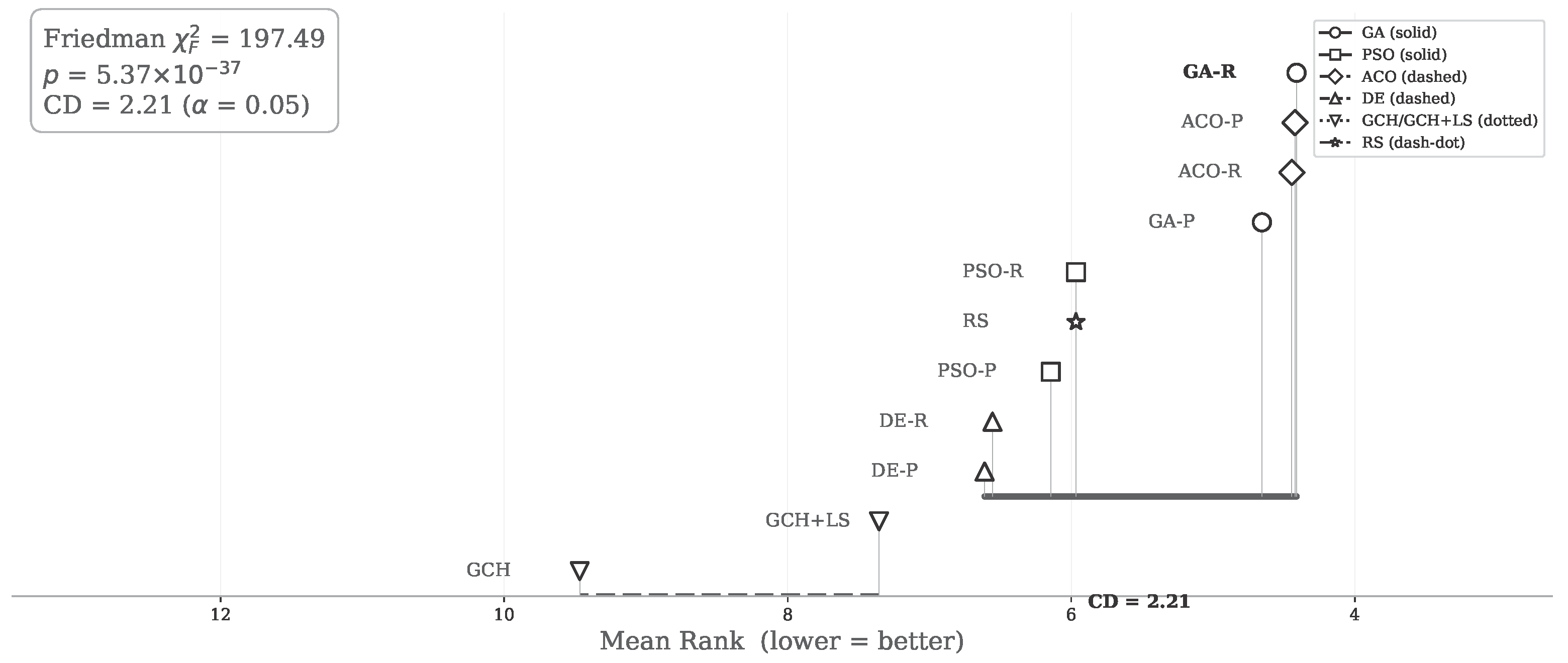
Table 9 presents the overall ranking. The Shapiro–Wilk test rejected normality for 9 of 11 algorithms ( p < 0.05 ). The Friedman test confirmed significant differences among algorithms ( χ F 2 = 197.49 , df = 10, p = 5.37 × 10 37 ), with a critical difference of C D = 2.21 . The eight metaheuristic variants and RS form a single homogeneous tier—no pairwise comparison among them reaches significance after Holm–Bonferroni correction under the present experimental design ( N = 45 instances, 10 runs each). GCH alone occupies the bottom tier ( p < 0.001 vs. all others).
Three subsidiary findings: (1) GCH achieves 84.2% of GA-R’s utilization in <0.1 s. (2) RS achieves U ¯ = 0.6235 , statistically indistinguishable from GA-R ( U ¯ = 0.6319 ), indicating the DBLF decoder accounts for 98.7% of the best metaheuristic’s utilization. (3) ACO achieves the highest absolute U ¯ (0.6325), but at 2.4× the cost of GA and 3.8× that of PSO/DE.

5.4.2. Optimality Analysis on Small Instances

Although the MILP formulation is computationally intractable for n 50 (Section 3.3), it remains solvable for small instances, providing an absolute performance reference. We generated 18 small instances ( n = 8 , 10 , 12 , 15 , 18 , 20 ; six problem sizes × three replicates) and solved each to proven optimality using the open-source CBC solver (1–17 s per instance). GA, RS, and GCH were then applied under the same protocol used in the main experiment (10,000 evaluations, three runs each).
GA and random search achieved the optimal solution on all 18 instances (optimality gap = 0 % in every case). GCH reached the optimum on 6 of 18 instances, with a mean optimality gap of 23.1% (standard deviation 29.0%, maximum 83.9%). This result establishes that, at scales where optimality can be verified, the metaheuristic-plus-DBLF pipeline recovers the global optimum. The finding also provides partial context for the 15.8% metaheuristic improvement over GCH reported on the benchmark: GCH can deviate from optimality by over 20 percentage points even at n = 20 , so an improvement of this magnitude is plausible and meaningful. The small instances are necessarily sparser than the benchmark (∼50–65% fill ratio vs. ∼90%) and do not exhibit the compatibility-driven ranking collapse documented in Section 5.4; extrapolation to n 50 should therefore be cautious.
Table 10 reports per-instance win counts. ACO-P won 33 of 45 instances (73.3%), yet 86.7% of instances produced ties (wins awarded under a 0.005 threshold). The homogeneous subsets identified by the Friedman test are shown in the CD diagram (Figure 1): the eight metaheuristics and RS form a single tier (T1).

5.4.3. Convergence Speed Analysis

Table 11 reports the number of evaluations required to reach the best solution during each run (lower values indicate faster convergence). ACO variants converge fastest (mean K 1230 ) and most consistently (lowest standard deviation), reflecting the constructive nature of ant-based search. GA variants require approximately 50% more evaluations (mean K 1800 ) and exhibit the widest variance, indicating greater run-to-run variability. PSO and DE occupy an intermediate position. RS exhausts the full budget; GCH + LS and GCH are deterministic, with zero variance across runs (Std K = 0 ). The convergence ordering (ACO < DE ≈ PSO < GA) differs from the final solution quality ordering, suggesting that faster convergence does not imply better final solutions in this problem class.

5.4.4. RQ2: Constraint Density Moderation Effect

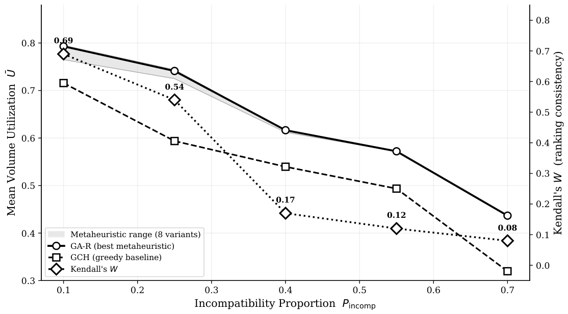
Kendall’s W declines monotonically from 0.69 to 0.08 as P incomp increases (Table 12). At P incomp = 0.10 , rankings are highly consistent ( W = 0.69 ), as observed in classical unconstrained 3D-BPP studies. At P incomp = 0.40 , consistency drops sharply ( W = 0.16 ). At P incomp = 0.70 , W = 0.08 —near the theoretical minimum—indicating that algorithm rankings at this density are dominated by instance-specific compatibility patterns rather than algorithmic differences. ACO variants achieve the highest mean at the two lowest constraint densities ( P incomp = 0.10 , 0.25 ), while GA-R achieves the highest mean at moderate-to-high densities ( P incomp 0.40 ). Figure 2 summarizes both effects in a single view: the gray band shows that all eight metaheuristic variants occupy a narrow utilization range regardless of P incomp , while Kendall’s W (right axis, diamond markers) declines from 0.69 to 0.08, confirming that constraint density, not algorithm choice, is the dominant performance driver.

5.4.5. RQ3: Constraint-Handling Strategy Comparison

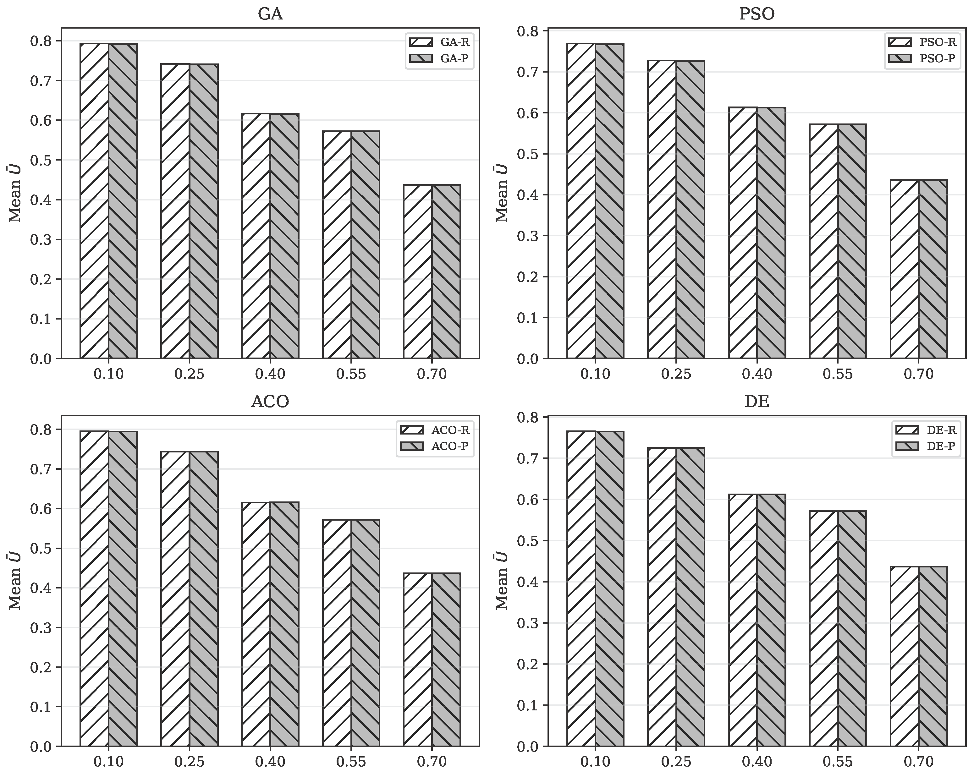
No pairwise comparison reaches significance (Table 13). The decoder’s internal compatibility filter prevents incompatible placements from entering any candidate solution, so both repair and penalty strategies operate on already-feasible solutions. The decoder-embedded hard filter is therefore the most practical mechanism among those tested: it guarantees feasibility, requires no tuning, and incurs zero per-generation overhead. This comparison is subject to a tuning asymmetry (the penalty coefficient λ was calibrated via iRace whereas repair operator parameters were fixed at their design values); this caveat is discussed further in Section 6. Figure 3 confirms that the repair and penalty variants produce nearly identical utilization across all constraint levels.

5.4.6. Distributional Analysis and Additional Stratifications

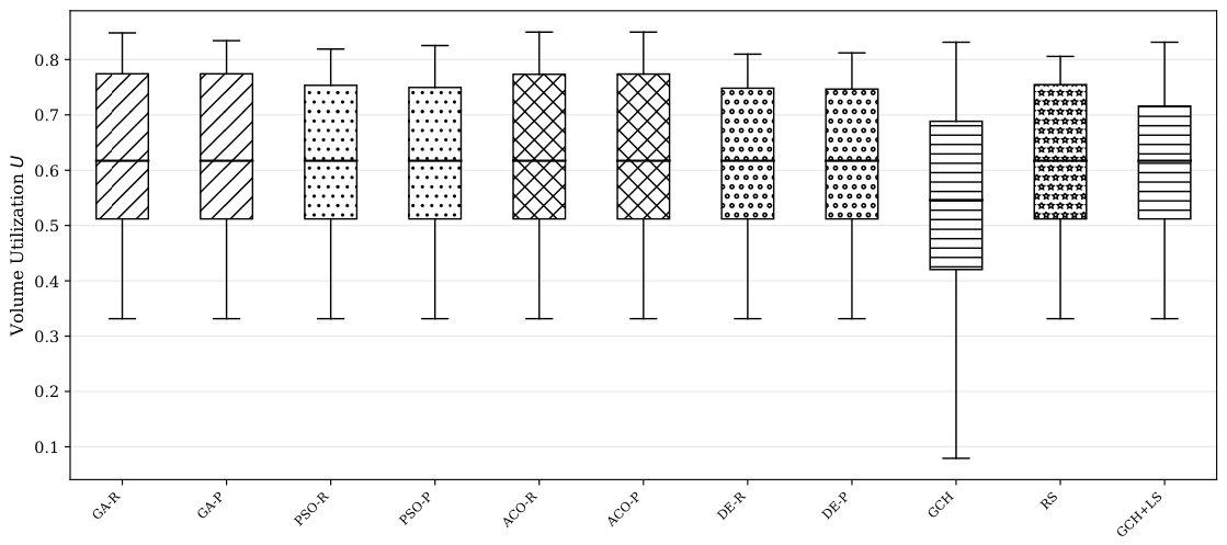
The boxplot (Figure 4) confirms the homogeneity of the metaheuristic tier: GA, PSO, ACO, and DE variants exhibit overlapping interquartile ranges, while GCH is clearly separated. RS achieves a median comparable to the metaheuristics, reinforcing the decoder-dominance interpretation. ACO variants exhibit slightly narrower variance, consistent with their incremental, compatibility-aware construction that reduces instance-to-instance variability.
Stratification by N types and θ size . Table 14 reports the best-performing algorithm when instances are stratified by item type count and size heterogeneity, with mean U ¯ shown in parentheses (complementing the P incomp stratification in Section 5.4).
The stratified results in Table 14 reveal that ACO overtakes GA as the dominant metaheuristic when N types 50 , consistent with ACO’s incremental construction scaling better to larger action spaces. Under high size heterogeneity, ACO-P achieves the highest absolute mean U ¯ (0.6744), suggesting that the combination of constructive search and compatibility-aware heuristics is particularly effective when item dimensions vary widely. GCH remains the worst performer across all strata, confirming that the rank ordering is largely invariant to N types and θ size , in contrast to the strong P incomp moderation documented in Section 5.4.

6. Discussion

6.1. The Decoder Dominance Hypothesis

Random search achieves 98.7% of the best metaheuristic’s performance and is statistically indistinguishable from it. This supports a DBLF-dominance hypothesis: the DBLF heuristic’s lexicographic priority rule produces near-optimal packings from almost any item ordering, and the metaheuristic contributes at most a 15.8% improvement over the greedy baseline. An alternative interpretation is that all four metaheuristics, when paired with the identical DBLF decoder and budget, converge to similarly valued regions of the DBLF-guided fitness landscape; the present experiment cannot distinguish between decoder dominance and fitness-landscape convergence. Testing this distinction would require varying the decoder itself—a natural direction for future work.
Our results reflect a broader pattern in the metaheuristics literature: stochastic search often derives its power from problem-specific components rather than the high-level search framework. In 3D constrained packing, the DBLF corner-point placement heuristic is that component; the choice of metaheuristic wrapper is secondary. Ali et al. (2022) [12] identified “constraint-aware algorithm comparison” as an open problem in their survey of 3D packing papers, and our benchmark directly addresses this gap by showing that constraint awareness at the decoder level suffices.

6.2. Constraint Density as a Moderator

The monotonic decline of Kendall’s W from 0.69 to 0.08 constitutes the paper’s central empirical finding. This metric captures inter-instance ranking consistency rather than mean differences alone, and its collapse reveals that constraint density—not algorithm design—is the primary performance moderator. At low P incomp , the problem approximates unconstrained 3D-BPP and the literature’s established hierarchy (GA ≈ ACO > PSO ≈ DE) carries over [4]. At high P incomp , rankings collapse because instance-specific compatibility patterns overwhelm any algorithmic signal.
This interaction—adding constraints changes which strategies are effective, not merely how hard the problem is—has not been documented in the BPPC literature. Prior work has focused on exact algorithms and lower bounds [7,8] without examining how conflict-graph density interacts with solution method performance. Our results suggest that structural properties of the compatibility matrix (cluster sizes, isolates) are more predictive of algorithm success than generic algorithmic features. Future BPPC work should therefore report constraint-density-stratified results as standard practice, and the benchmark instances released with this paper provide a testbed for such investigations.
The present findings both align with and depart from the existing literature. The dominance of GA and ACO over PSO and DE at low constraint densities is consistent with Gonçalves and Resende [4], who reported GA-based approaches to be effective for unconstrained container loading. The collapse of this hierarchy at moderate-to-high P incomp and the statistical indistinguishability of random search from all metaheuristics are, however, novel observations not reported in prior 3D-BPP studies—a discrepancy that likely reflects the fact that earlier work did not systematically vary constraint density or report constraint-stratified rankings. The finding that decoder-embedded filtering renders repair and penalty strategies equivalent contrasts with the BPPC literature, where explicit constraint handling is essential because no geometric placement heuristic pre-filters incompatible items. This divergence carries a methodological implication: findings from one-dimensional BPPC studies do not automatically transfer to the 3D setting, where the placement decoder supplies an additional layer of constraint awareness.

6.3. Implications for Algorithm Design

Two practical recommendations follow from these results. First, for problems where categorical constraints can be checked at placement time with negligible overhead, a decoder-embedded hard filter is the optimal mechanism. It guarantees feasibility, requires no parameter tuning, and adds zero per-generation cost. By contrast, explicit repair and penalty strategies add implementation complexity without empirical benefit—consistent with Rahimi et al. (2023) [10], who argue that constraint-handling strategies should be tailored to problem structure rather than applied generically.
Second, when the target constraint density is known in advance, algorithm selection can be guided by P incomp -stratified rankings: at low density, any metaheuristic suffices; at high density, ACO’s incremental, compatibility-aware construction provides a consistent but modest advantage. These findings underscore the value of systematic benchmarking: design choices that appear theoretically consequential may be rendered moot by problem-specific heuristics, while genuinely impactful factors such as constraint density remain invisible to single-algorithm studies.

6.4. Limitations

Internal validity. All experiments share a common codebase; any implementation bias is conservative in direction, since relative comparisons are less sensitive to shared components than absolute performance. All algorithms used default parameters without automated tuning. This ensures fairness but may understate the performance of algorithms whose defaults are further from optimal. The continuous-to-discrete mapping used by PSO and DE ( π = argsort ( x ) ) introduces an additional concern: nearby points in the continuous search space may map to identical permutations, reducing effective search diversity. Additionally, the constraint-handling comparison introduced a tuning asymmetry: the penalty coefficient λ was calibrated via iRace, whereas the repair operator parameters (e.g., re-insertion order) were fixed. This may disadvantage the repair strategy relative to the tuned penalty. The finding that penalty and repair are statistically equivalent should therefore be interpreted as conservative: even with a tuning advantage favoring the penalty strategy, it does not outperform repair. Symmetric tuning of both strategies would be required for a fully balanced comparison.
External validity. Instances were generated synthetically under distributional assumptions that have not been calibrated against empirical logistics data. Results may not generalize to real-world loading scenarios with different item dimension distributions or compatibility structures.
Statistical power. With 10 runs per configuration and 9 instances per P incomp stratum, the design may lack power to detect small effect sizes. The critical difference ( C D = 2.21 , reflecting N = 45 instances) is relatively wide, so moderate differences within the metaheuristic tier may be masked. Replication with all 225 generated instances would narrow the CD and enable finer discrimination. However, the qualitative pattern—a stark gap between the metaheuristic-plus-RS tier and GCH, and the collapse of ranking consistency at high P incomp —would persist regardless of sample size.
Practical significance. Although the eight metaheuristic variants and RS are statistically indistinguishable, the observed 2.5% relative difference between the best (ACO-R: U ¯ = 0.6325 ) and worst (DE-P: U ¯ = 0.6223 ) metaheuristic may carry economic significance in high-volume logistics operations where small percentage improvements translate into substantial cost savings. We therefore distinguish between statistical indistinguishability (an artifact of the present experimental design) and practical equivalence (which would require a domain-specific cost–benefit analysis beyond the scope of this benchmark). A study with larger sample sizes or all 225 generated instances would be required to determine whether the 2.5% difference reflects a real effect or sampling noise.
Scope. This benchmark is limited to population-based metaheuristics. Single-solution methods (simulated annealing, tabu search, iterated local search) and hybrid approaches such as BRKGA remain to be evaluated. Furthermore, the absence of optimal solutions (the MILP is intractable for n 50 ) means the 15.8% improvement over GCH cannot be contextualized against a known upper bound; optimal solutions for smaller instances ( n 20 ) would anchor the absolute performance scale.

7. Conclusions

This paper introduced the 3D-SBPP-CC, a problem that couples 3D geometric packing with categorical incompatibility constraints, and conducted a systematic benchmark of four population-based metaheuristics under a matched computational budget. The key findings are as follows.
Problem formalization. We presented a complete MILP formulation of the 3D-SBPP-CC, encoding pairwise compatibility as the linear inequality s i + s j 1 + m c i , c j , and proved the problem strongly NP-hard via independent reductions from 3D-SBPP and BPPC.
Systematic benchmark. Under a uniform budget of 10,000 fitness evaluations, the eight metaheuristic variants and random search form a single statistically homogeneous tier ( χ F 2 = 197.49 , C D = 2.21 , p < 10 36 ). The DBLF decoder, not the metaheuristic, governs packing quality: RS achieves 98.7% of GA-R’s utilization, and GCH achieves 84.2% in under 0.1 s.
Benchmark instances. We publicly release 225 stratified instances ( 5 × 3 × 3 factorial design) with a documented generator, providing a reproducible testbed for constrained 3D packing with categorical incompatibility rules.
Constraint-density moderation. Kendall’s W declines monotonically from 0.69 to 0.08 as P incomp increases, confirming that constraint density is the primary performance moderator. Decoder-embedded compatibility filtering renders explicit repair and penalty strategies redundant ( p > 0.05 at all constraint levels).
Future work should pursue several directions. First, systematically varying the decoder (e.g., comparing DBLF against Bottom-Left, Best-Fit, or learning-based placement rules) would test whether the DBLF-dominance finding generalizes and distinguish decoder dominance from fitness-landscape convergence. Second, obtaining optimal solutions via MILP solvers on small instances ( n 20 ) would anchor the absolute performance scale and contextualize the 15.8% improvement over GCH. Third, calibrating instance distributions against empirical logistics data would strengthen external validity and identify which constraint-density regimes are most common in practice. Additional directions include extending the benchmark to single-solution methods and BRKGA [4], incorporating further practical constraints [25], pursuing multi-objective formulations trading utilization against safety margins, and exploring learning-augmented construction heuristics [30] that may surpass the hand-designed DBLF rule.

Author Contributions

Conceptualization, Y.J. and Z.X.; methodology, Y.J.; software, Y.J.; validation, Y.J., Z.X., T.L., Q.Y. and K.Y.; formal analysis, Y.J.; investigation, Y.J., Q.Y. and K.Y.; data curation, Y.J.; writing—original draft preparation, Y.J.; writing—review and editing, Z.X., T.L., Q.Y. and K.Y.; visualization, Y.J.; supervision, Z.X. All authors have read and agreed to the published version of the manuscript.

Funding

This research received no external funding.

Data Availability Statement

The source code, benchmark instances, and experimental results presented in this study are openly available at https://doi.org/10.5281/zenodo.21866696.

Conflicts of Interest

The authors declare no conflicts of interest.

Abbreviations

3D-BPPThree-Dimensional Bin Packing Problem
3D-SBPP-CC3D Single Bin Packing Problem with Categorical Compatibility Constraints
ACOAnt Colony Optimization
BPPCBin Packing Problem with Conflicts
CDCritical Difference
DBLFDeepest-Bottom-Left-Fill
DEDifferential Evolution
GAGenetic Algorithm
GCHGreedy Constructive Heuristic
MILPMixed-Integer Linear Programming
PSOParticle Swarm Optimization
RPDRelative Percentage Deviation
RSRandom Search

References

  1. Wäscher, G.; Haußner, H.; Schumann, H. An improved typology of cutting and packing problems. Eur. J. Oper. Res. 2007, 183, 1109–1130. [Google Scholar] [CrossRef] [Scilit]
  2. Bortfeldt, A.; Wäscher, G. Constraints in container loading: A state-of-the-art review. Eur. J. Oper. Res. 2013, 229, 1–20. [Google Scholar] [CrossRef] [Scilit]
  3. Martello, S.; Pisinger, D.; Vigo, D. The three-dimensional bin packing problem. Oper. Res. 2000, 48, 256–267. [Google Scholar] [CrossRef] [Scilit]
  4. Gonçalves, J.F.; Resende, M.G.C. A parallel multi-population biased random-key genetic algorithm for a container loading problem. Comput. Oper. Res. 2012, 39, 179–190. [Google Scholar] [CrossRef] [Scilit]
  5. Francescatto, M.; Neuenfeldt Junior, A. Two-dimensional bin packing, cutting stock, and open dimension problems: A survey of practical requirements. Comput. Oper. Res. 2025, 183, 107209. [Google Scholar] [CrossRef] [Scilit]
  6. UN Model Regulations. United Nations Model Regulations on the Transport of Dangerous Goods, 23rd rev. ed.; United Nations: New York, NY, USA, 2023. [Google Scholar]
  7. Gendreau, M.; Laporte, G.; Semet, F. Heuristics and lower bounds for the bin packing problem with conflicts. Comput. Oper. Res. 2004, 31, 347–358. [Google Scholar] [CrossRef] [Scilit]
  8. Muritiba, A.E.F.; Iori, M.; Malaguti, E.; Toth, P. Algorithms for the bin packing problem with conflicts. INFORMS J. Comput. 2010, 22, 401–415. [Google Scholar] [CrossRef] [Scilit]
  9. Zhong, X.; Ren, H.; Wang, D.; Wei, D. Research and optimization of container explosives packing problem based on hybrid heuristic algorithm. Navig. China 2025, 48, 166–174. [Google Scholar]
  10. Rahimi, I.; Gandomi, A.H.; Chen, F.; Mezura-Montes, E. A review on constraint handling techniques for population-based algorithms: From single-objective to multi-objective optimization. Arch. Comput. Methods Eng. 2023, 30, 2181–2209. [Google Scholar] [CrossRef] [Scilit]
  11. Qiao, K.; Liang, J.; Yu, K.; Yue, C.; Lin, H.; Zhang, D.; Qu, B. Evolutionary constrained multiobjective optimization: Scalable high-dimensional constraint benchmarks and algorithm. IEEE Trans. Evol. Comput. 2024, 28, 965–979. [Google Scholar] [CrossRef] [Scilit]
  12. Ali, S.; Ramos, A.G.; Carravilla, M.A.; Oliveira, J.F. On-line three-dimensional packing problems: A review of off-line and on-line solution approaches. Comput. Ind. Eng. 2022, 168, 108122. [Google Scholar] [CrossRef] [Scilit]
  13. Dahmani, N.; Nazir, A.; Taleb, I.; Bukhari, S.M.S. Reinforcement learning based intelligent optimisation for bin packing problems: A review. Array 2025, 28, 100616. [Google Scholar] [CrossRef] [Scilit]
  14. Zhang, B.; Yao, Y.; Kan, H.K.; Luo, W. A GAN-based genetic algorithm for solving the 3D bin packing problem. Sci. Rep. 2024, 14, 7775. [Google Scholar] [CrossRef] [Scilit] [PubMed]
  15. Liu, Y.; Jiang, X. Dynamic feedback algorithm based on spatial corner fitness for solving the three-dimensional multiple bin-size bin packing problem. Complex Intell. Syst. 2024, 10, 4055–4081. [Google Scholar] [CrossRef] [Scilit]
  16. Ananno, A.A.; Ribeiro, L. A multi-heuristic algorithm for multi-container 3-D bin packing problem optimization using real world constraints. IEEE Access 2024, 12, 42105–42130. [Google Scholar] [CrossRef] [Scilit]
  17. Ali, S.; Ramos, A.G.; Oliveira, J.F. Static stability versus packing efficiency in online three-dimensional packing problems: A new approach and a computational study. Comput. Oper. Res. 2025, 178, 107005. [Google Scholar] [CrossRef] [Scilit]
  18. Ambrosino, D.; Sciomachen, A. Using a bin packing approach for stowing hazardous containers into containerships. In Optimized Packings with Applications; Fasano, G., Pinter, J.D., Eds.; Springer: Cham, Switzerland, 2015; pp. 1–18. [Google Scholar]
  19. Parreño, F.; Pacino, D.; Alvarez-Valdes, R. A GRASP algorithm for the container stowage slot planning problem. Transp. Res. Part E 2016, 94, 141–157. [Google Scholar] [CrossRef] [Scilit]
  20. Kamieniev, K.; Kamienieva, A.; Tsymbal, M. Construction of a mathematical model and a method for arranging hazardous cargoes on a containership. East.-Eur. J. Enterp. Technol. 2019, 6, 20–27. [Google Scholar] [CrossRef] [Scilit]
  21. Jia, B.; Fagerholt, K. Step-wise stowage planning of roll-on roll-off ships transporting dangerous goods. Marit. Transp. Res. 2021, 2, 100029. [Google Scholar] [CrossRef] [Scilit]
  22. Santos, L.F.O.M.; Iwayama, R.S.; Cavalcanti, L.B.; Turi, L.M.; Morais, F.E.S.; Mormilho, G.; Cunha, C.B. A variable neighborhood search algorithm for the bin packing problem with compatible categories. Expert Syst. Appl. 2019, 124, 209–225. [Google Scholar] [CrossRef] [Scilit]
  23. Rodrigues, G.A.; Cunha, C.B.; Guarino Neto, L.; Vidal Vieira, J.G. An adaptive large neighborhood search metaheuristic for the Generalized Bin Packing problem with incompatible categories. Comput. Ind. Eng. 2023, 185, 109586. [Google Scholar] [CrossRef] [Scilit]
  24. Tsao, Y.-C.; Tai, J.-Y.; Vu, T.-L.; Chen, T.-H. Multiple bin-size bin packing problem considering incompatible product categories. Expert Syst. Appl. 2024, 247, 123340. [Google Scholar] [CrossRef] [Scilit]
  25. do Nascimento, O.C.B.; Queiroz, T.A.; Junqueira, L. Practical constraints in the container loading problem: Comprehensive formulations and exact algorithm. Comput. Oper. Res. 2021, 128, 105186. [Google Scholar] [CrossRef] [Scilit]
  26. Dorigo, M.; Gambardella, L.M. Ant colony system: A cooperative learning approach to the traveling salesman problem. IEEE Trans. Evol. Comput. 1997, 1, 53–66. [Google Scholar] [CrossRef] [Scilit]
  27. López-Ibáñez, M.; Dubois-Lacoste, J.; Pérez Cáceres, L.; Birattari, M.; Stützle, T. The irace package: Iterated racing for automatic algorithm configuration. Oper. Res. Perspect. 2016, 3, 43–58. [Google Scholar] [CrossRef] [Scilit]
  28. Demšar, J. Statistical comparisons of classifiers over multiple data sets. J. Mach. Learn. Res. 2006, 7, 1–30. [Google Scholar]
  29. Wobbrock, J.O.; Findlater, L.; Gergle, D.; Higgins, J.J. The aligned rank transform for nonparametric factorial analyses using only ANOVA procedures. In Proceedings of the SIGCHI Conference on Human Factors in Computing Systems (CHI ’11); ACM: New York, NY, USA, 2011; pp. 143–146. [Google Scholar]
  30. González-San-Martín, J.; Cruz-Reyes, L.; Dorronsoro, B.; Fraire-Huacuja, H.J.; Balderas-Jaramillo, F.A.; Quiroz-Castellanos, M.; Rangel-Valdez, N. Deep study on the application of machine learning in bin packing problems. Comput. Sist. 2024, 28, 1275–1290. [Google Scholar] [CrossRef] [Scilit]
Figure 1. Critical difference diagram ( C D = 2.21 , Friedman p < 10 36 ).
Algorithms 19 00707 g001
Figure 2. Mean volume utilization and Kendall’s W by incompatibility proportion.
Algorithms 19 00707 g002
Figure 3. Penalty versus repair comparison.
Algorithms 19 00707 g003
Figure 4. Distribution of volume utilization.
Algorithms 19 00707 g004
Table 1. Comparison of the present work with related studies.   ✓ = feature present; – = feature absent. The entry of the present work is shown in bold.
StudyProb.Compat.MethodMulti-MethodC-H StrategyPublic Data
Martello et al. [3]3DExact (branch-and-bound)
Gendreau et al. [7]1DExact + 6 heuristicsConflicts as bin-assignment constraints
Muritiba et al. [8]1DExact (branch-and-price)Conflict graph embedded in formulation
Ambrosino and Sciomachen [18]3DHeuristic (bin packing approach)IMDG segregation as slot constraints
Parreño et al. [19]3DMetaheuristic (GRASP)IMO separation rules in IP formulation
Kamieniev et al. [20]3DExact (Boolean ILP)IMDG segregation constraints
Santos et al. [22]1DMetaheuristic (VNS)Category conflicts in neighborhoods
Jia and Fagerholt [21]3DExact (MIP, step-wise)IMDG segregation in MIP
do Nascimento et al. [25]3DExact (ILP + CP)Conflicting items as constraints
Rodrigues et al. [23]1DMetaheuristic (ALNS)Category constraints in destroy/repair
Tsao et al. [24]3DHybrid (SA + GA)Categories handled in carton configuration
Zhong et al. [9]3DHybrid (GA–PSO)Explosive compatibility fitting
This work3D4 metaheuristics × 2 strategies + 3 baselinesPenalty vs. repair vs. decoder filter (compared)
Table 2. The six orthogonal orientations.
ox-Axisy-Axisz-Axis
1 l i w i h i
2 l i h i w i
3 w i l i h i
4 w i h i l i
5 h i l i w i
6 h i w i l i
Table 3. Summary of notation.  Group headers are shown in italics.
SymbolDomainDescription
Sets and indices
I ; i, j { 1 , , n } Set of items
G ; g, h13 hazard classes (Table 4)Compatibility categories
O ; o { 1 , , 6 } Orthogonal orientations (Table 2)
Parameters
L , W , H Z + (cm)Container interior dimensions; V C = L · W · H
l i , w i , h i Z + (cm)Item i dimensions; v i = l i · w i · h i
c i G Category of item i
l i o , w i o , h i o Z + (cm)Dimensions of item i after rotation o
m g h { 0 , 1 } 1 if categories g and h are co-loadable
M Z + max { L , W , H } + 1 (big-M)
Decision variables
x i , y i , z i R + Placement coordinates of item i
s i { 0 , 1 } 1 if item i is packed
δ i o { 0 , 1 } 1 if item i is assigned orientation o
α i j 1 , , α i j 6 { 0 , 1 } Non-overlap auxiliary binaries for pair ( i , j )
Table 4. Categorical compatibility matrix (1 = compatible, 0 = incompatible). Rows and columns index the 13 compatibility categories of G defined in Section 3.
ABCDEFGHJKLNS
A1000000000000
B0111110000001
C0111110000001
D0111110000001
E0111110000001
F0111110000001
G0000001111001
H0000001111001
J0000001111001
K0000001111001
L0000000000100
N0000000000011
S0111111111011
Table 5. Per-generation complexity and key parameters.
AlgorithmComplexitySizeKey Parameters
GA O ( N · D ) 100OX crossover, p mut = 0.10 , elitism 5
PSO O ( N · D ) 100 w = 0.7 , c 1 = c 2 = 2.0 , global-best topology
ACO O ( N · D + N · n 2 ) 50 ρ = 0.10 , q 0 = 0.10 , 2-opt depth 10
DE O ( N · D ) 100 F = 0.7 , C R = 0.7 , rand-to-best/1/bin
Table 6. Unified metaheuristic framework for the 3D-SBPP-CC. Shared components are identical across all configurations; algorithm-specific components are described compactly for each metaheuristic. Algorithm labels within cells are set in bold.
StepScopeDescription
EncodingSharedPermutation π of { 1 , , n } plus orientation vector o { 1 , , 6 } n
InitializationAlgorithm-specificGA/PSO/DE: random permutations and orientations. ACO: pheromone matrix τ[i][] initialized to τ 0 = 1 / ( n · U GCH )
DecodingSharedDBLF corner-point placement with decoder-embedded compatibility filter (Section 4)
EvaluationSharedVolume utilization U; modified by penalty term λ · g ( P ) or repair pass depending on constraint-handling variant
SelectionAlgorithm-specificGA: tournament (size 3, elitism top-5). DE: one-to-one (trial vs. target). PSO: personal best + global best. ACO: pseudo-random-proportional ( q 0 = 0.10 )
VariationAlgorithm-specificGA: OX crossover + mutation ( p mut = 0.10 ). DE: rand-to-best/1/bin ( F = 0.7 , C R = 0.7 ). PSO: velocity update ( w = 0.7 , c 1 = c 2 = 2.0 ). ACO: pheromone-guided construction + 2-opt (depth 10)
ReplacementAlgorithm-specificGA: elitism (top-5 preserved). DE/PSO: one-to-one (trial replaces target if better). ACO: global pheromone update on best-so-far ( ρ = 0.10 )
TerminationShared10,000 fitness evaluations or 1000 without improvement
Table 7. Algorithm configurations.
IDAlgorithmConstraint Handling
GA-RGenetic AlgorithmRepair operator
GA-PPenalty function
PSO-RParticle Swarm OptimizationRepair operator
PSO-PPenalty function
ACO-RAnt Colony OptimizationRepair operator
ACO-PPenalty function
DE-RDifferential EvolutionRepair operator
DE-PPenalty function
GCHGreedy Constructive HeuristicHard filter
RSRandom SearchHard filter
GCH + LSGreedy + Local SearchHard filter
Table 8. Summary statistics of the 45 benchmark instances used in the main experiment.
ParameterMinMaxMean
Total items ( N total )5911774.8
Item types ( N types )208050.0
Fill ratio0.801.201.00
Groups used (out of 13)7129.8
P incomp (actual)0.100.700.40
Table 9. Overall ranking across 45 instances (4950 runs).
Algorithm U ¯ s U RPD ¯ (%) T ¯ (s) S global
GA-R0.63190.14301.03217.60.9710
GA-P0.63150.14251.08218.80.9687
ACO-R0.63250.14410.96509.20.9400
ACO-P0.63250.14420.95519.40.9389
PSO-R0.62370.13402.04133.60.9356
PSO-P0.62310.13342.12137.70.9317
DE-R0.62230.13262.21134.70.9277
DE-P0.62230.13252.22137.00.9273
GCH + LS0.61260.12513.46102.20.8773
RS0.62350.13372.06850.40.8502
GCH0.53240.184217.030.10.4000
Table 10. Per-instance win counts (wins awarded under a 0.005 tie threshold; 39 of 45 instances produced ties).
AlgorithmWinsShare
ACO-P3373.3%
GA-R511.1%
ACO-R48.9%
GA-P36.7%
PSO-R00.0%
PSO-P00.0%
DE-R00.0%
DE-P00.0%
RS00.0%
GCH00.0%
GCH + LS00.0%
Table 11. Evaluations to best-found solution (K), averaged over 10 runs and 45 instances.
AlgorithmMean KMedian KStd K
ACO-P12241000330
ACO-R12401000365
DE-R13961100393
DE-P14301100469
PSO-P14361100482
PSO-R14421100476
GA-R18071145918
GA-P18201145976
RS10,00010,0000
GCH + LS100110010
GCH110
Table 12. Stratified ranking by P incomp .
P incomp Algorithm with Highest Mean U ¯ U ¯ best Metaheuristic U ¯ RangeKendall’s W
0.10ACO-R0.7950[0.7650, 0.7950]0.694
0.25ACO-P0.7437[0.7251, 0.7437]0.543
0.40GA-R0.6165[0.6122, 0.6165]0.165
0.55GA-R0.5721[0.5720, 0.5721]0.121
0.70GA-R0.4367[0.4367, 0.4367]0.077
Note: All eight metaheuristic variants and RS are statistically indistinguishable at every P incomp level (Friedman post hoc, Holm-corrected p > 0.05 ). The “highest mean” designation is descriptive only and does not imply statistical superiority. The narrow U ¯ ranges confirm the paper’s finding of algorithmic homogeneity.
Table 13. Penalty vs. repair: paired Wilcoxon p-values.
Algorithm P incomp
0.100.250.400.550.70
GA0.5700.3121.0001.0001.000
PSO0.7340.4381.0001.0001.000
ACO1.0001.0001.0001.0001.000
DE0.8200.6881.0001.0001.000
Table 14. Best algorithm by N types and θ size .
FactorLevelBest Algorithm U ¯ best
N types 20GA-R0.6457
50ACO-R0.6058
80ACO-R0.6487
θ size lowGA-P0.6106
mediumACO-R0.6161
highACO-P0.6744
Disclaimer/Publisher’s Note: The statements, opinions and data contained in all publications are solely those of the individual author(s) and contributor(s) and not of MDPI and/or the editor(s). MDPI and/or the editor(s) disclaim responsibility for any injury to people or property resulting from any ideas, methods, instructions or products referred to in the content.