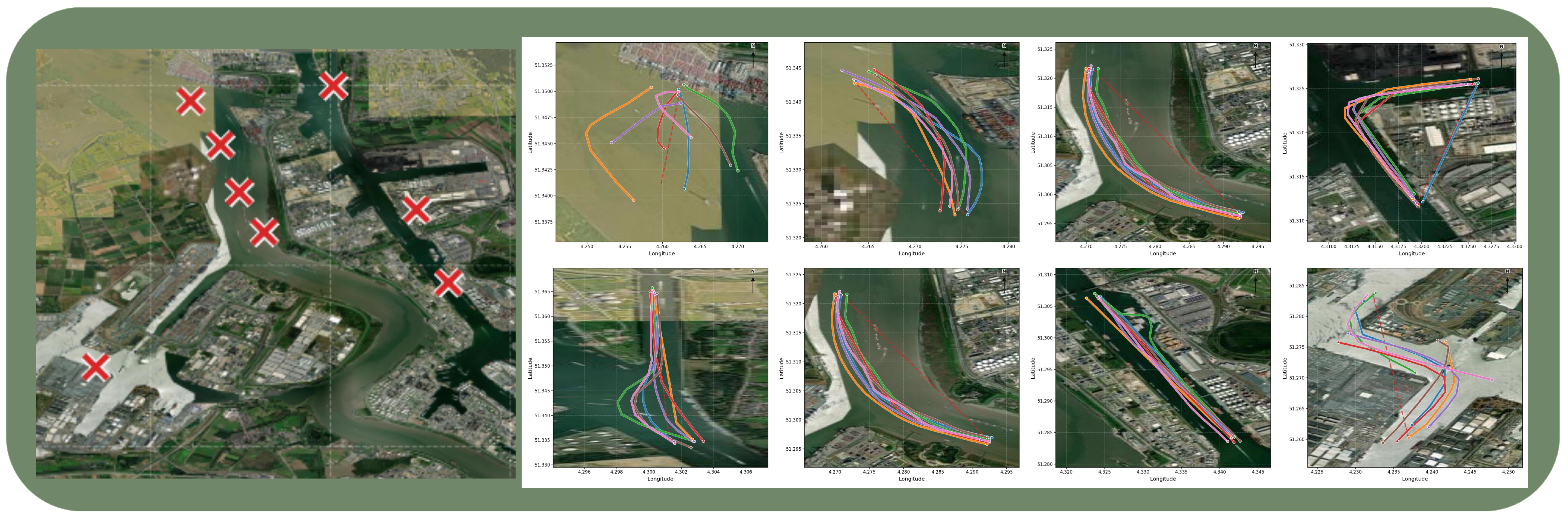
Figure 1.
Examples of trajectories for selected real-world gaps in the Port of Antwerp. The left panel marks the locations of eight selected real AIS gaps (red x markers). The right panels visualize, for each gap case, trajectories with similar start and end locations and comparable speed in different colours; the dashed red segments connect the two points of a gap.
Figure 1.
Examples of trajectories for selected real-world gaps in the Port of Antwerp. The left panel marks the locations of eight selected real AIS gaps (red x markers). The right panels visualize, for each gap case, trajectories with similar start and end locations and comparable speed in different colours; the dashed red segments connect the two points of a gap.
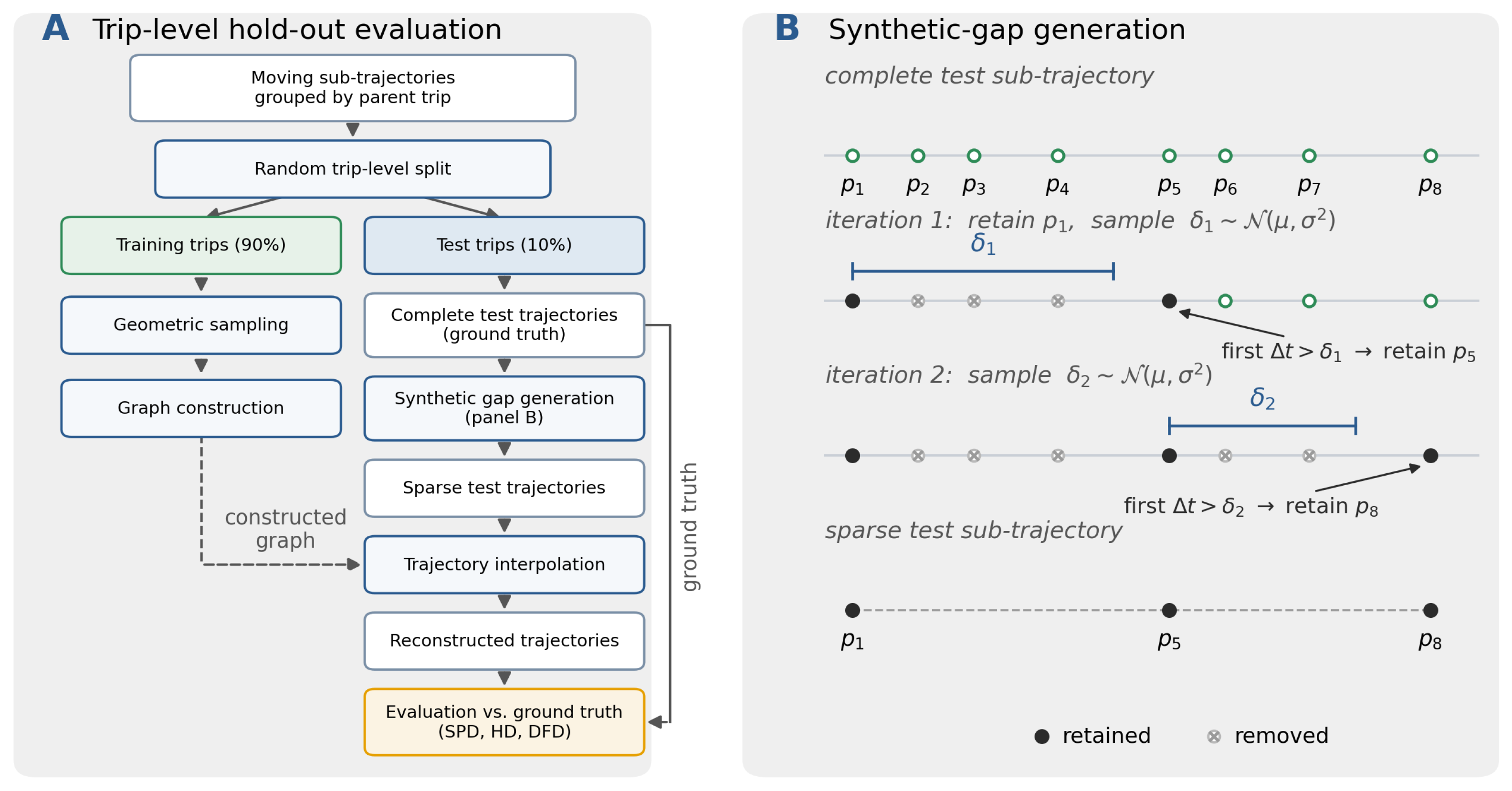
Figure 2.
Trip-level hold-out evaluation and synthetic-gap generation workflow. (A) Vessel trips were randomly assigned into training and test partitions. The training trajectories, following geometric sampling, were used for graph construction, whereas the complete test trajectories served as the ground truth for evaluation. The sparse test trajectories (see panel (B)) were used as input to the interpolation methods. (B) Given a trajectory (green dots), starting from a retained observation (black), a gap-duration threshold was sampled. Intermediate observations were removed (grey) until the first observation whose temporal difference from the retained observation exceeds was reached. That observation was retained (black), and the procedure was repeated until the end of the sub-trajectory. The last point of a given trajectory was always retained.
Figure 2.
Trip-level hold-out evaluation and synthetic-gap generation workflow. (A) Vessel trips were randomly assigned into training and test partitions. The training trajectories, following geometric sampling, were used for graph construction, whereas the complete test trajectories served as the ground truth for evaluation. The sparse test trajectories (see panel (B)) were used as input to the interpolation methods. (B) Given a trajectory (green dots), starting from a retained observation (black), a gap-duration threshold was sampled. Intermediate observations were removed (grey) until the first observation whose temporal difference from the retained observation exceeds was reached. That observation was retained (black), and the procedure was repeated until the end of the sub-trajectory. The last point of a given trajectory was always retained.
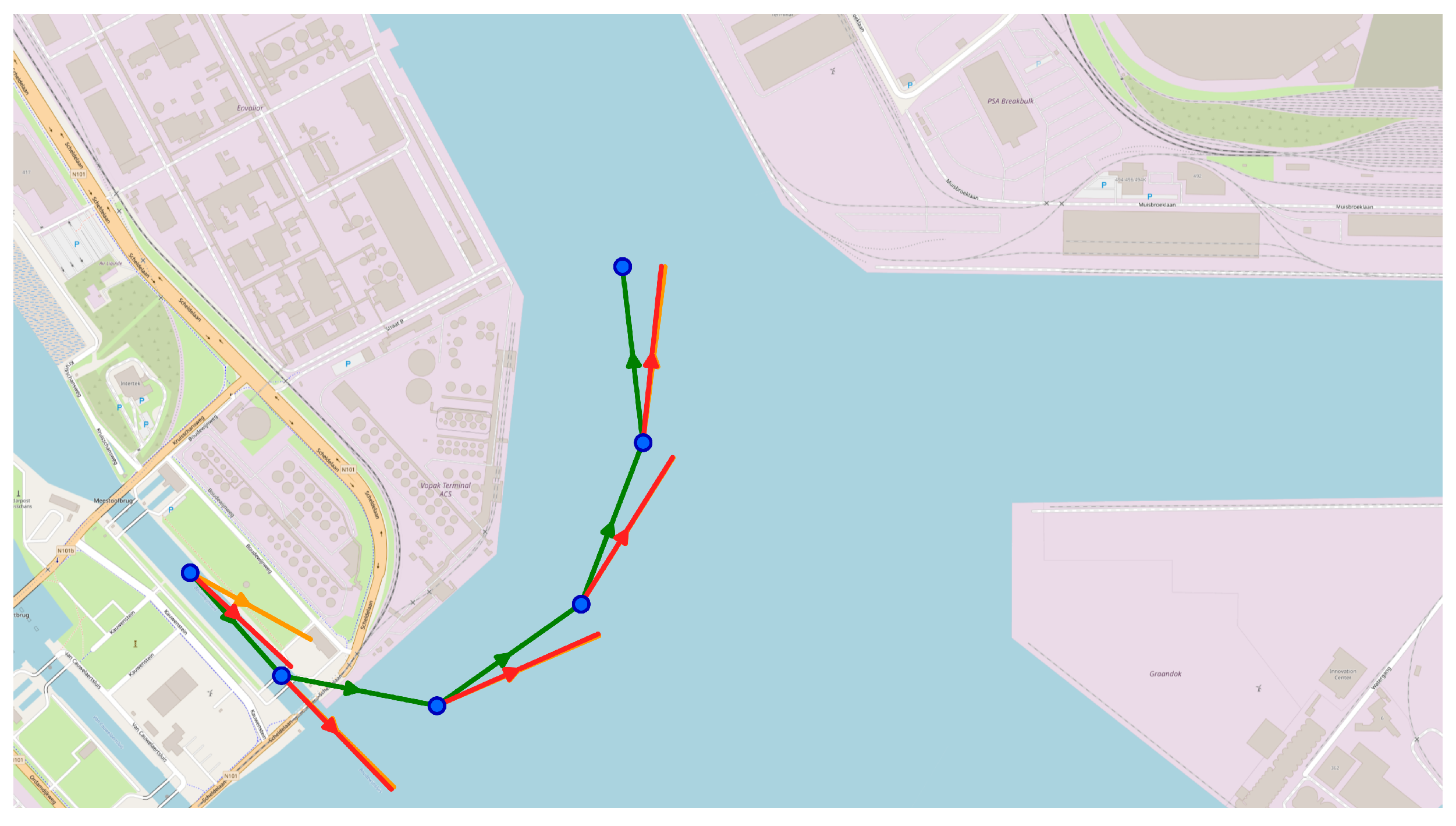
Figure 3.
Difference between true heading, course over ground, and calculated heading. A sub-trajectory illustrating the directions of true heading (red line), course over ground (orange line), and calculated heading (green line).
Figure 3.
Difference between true heading, course over ground, and calculated heading. A sub-trajectory illustrating the directions of true heading (red line), course over ground (orange line), and calculated heading (green line).
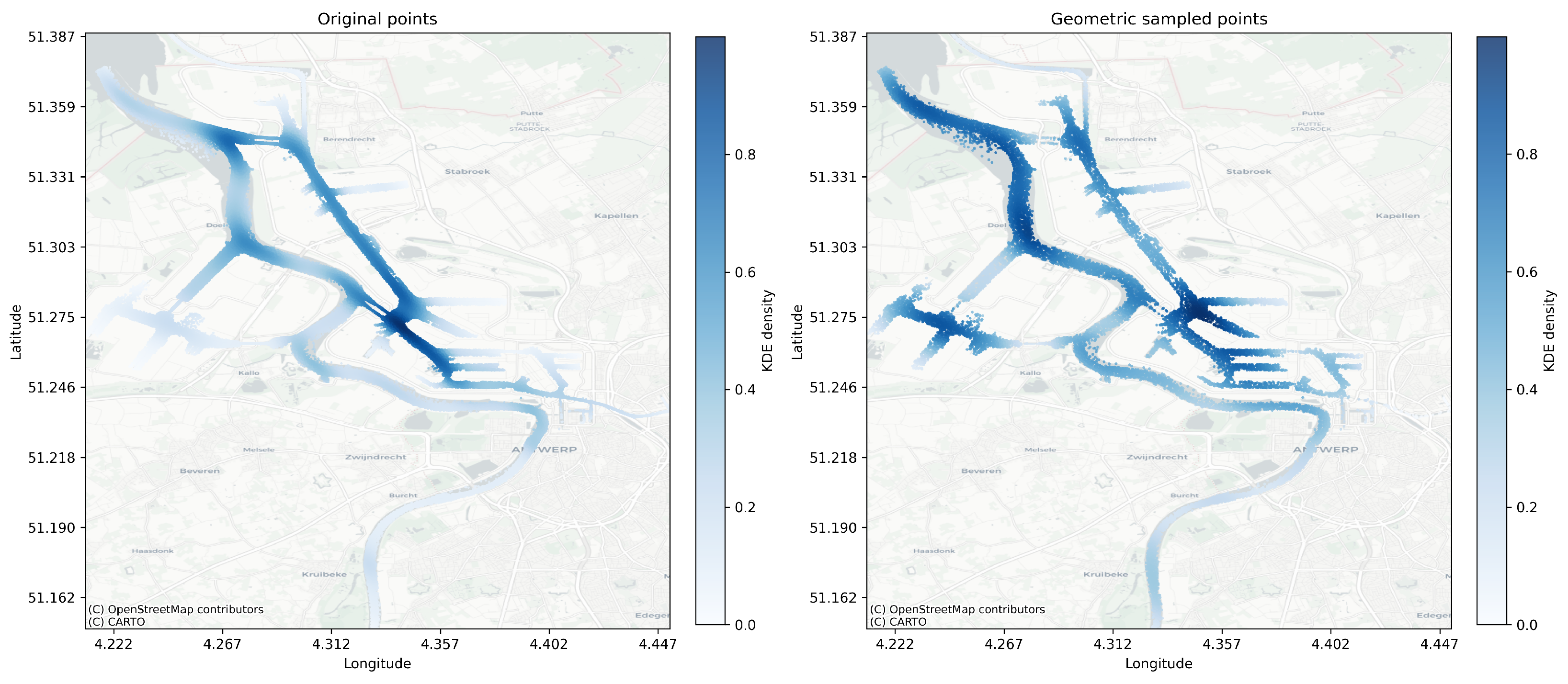
Figure 4.
Geometric sampling adjusts spatial density distribution in AIS data. This figure illustrates the spatial density difference following the application of geometric sampling to AIS data. In both plots, darker shades of blue indicate higher point densities, while lighter shades indicate lower densities. The left plot illustrates the spatial density of the original data from the training set. The right plot demonstrates the impact of geometric sampling.
Figure 4.
Geometric sampling adjusts spatial density distribution in AIS data. This figure illustrates the spatial density difference following the application of geometric sampling to AIS data. In both plots, darker shades of blue indicate higher point densities, while lighter shades indicate lower densities. The left plot illustrates the spatial density of the original data from the training set. The right plot demonstrates the impact of geometric sampling.
Figure 5.
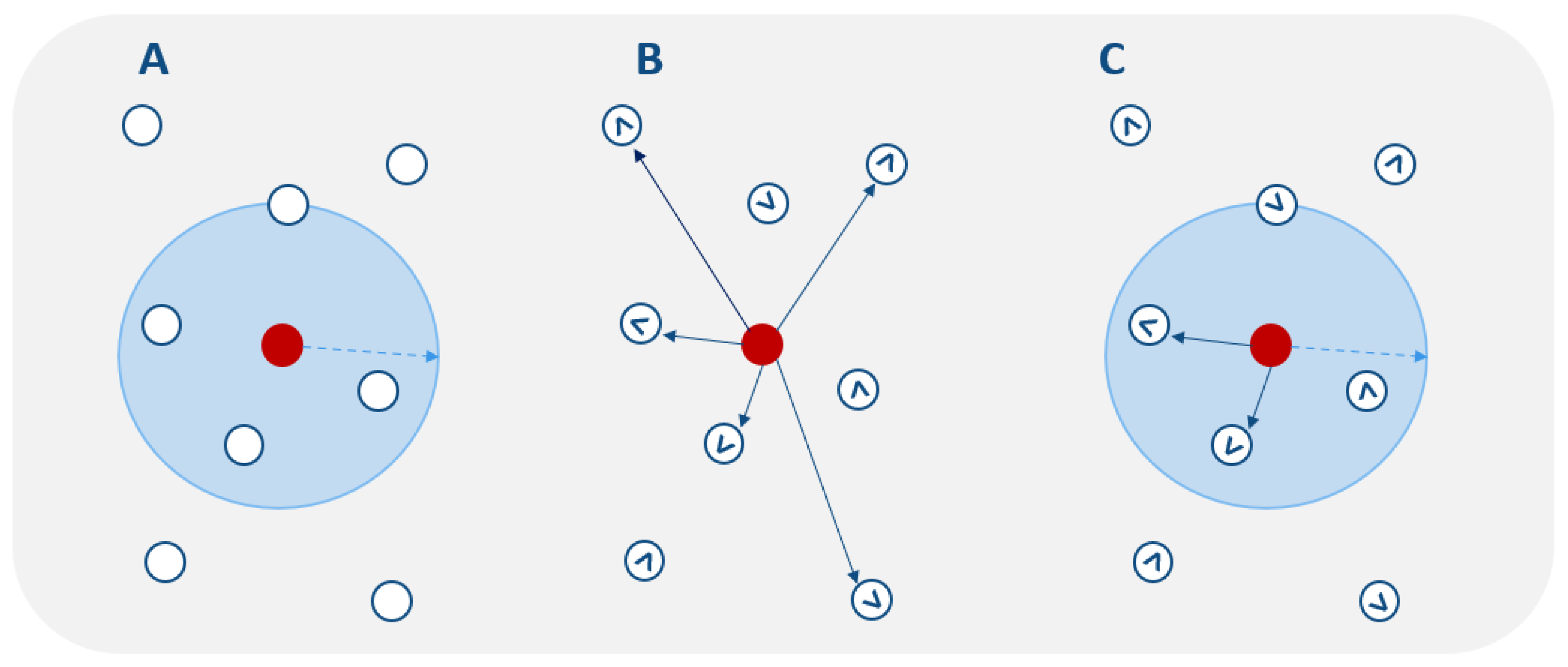
Visualization of DAISTIN’s edge construction criteria. (A) Neighbourhood criterion: only nodes within a predefined spatial radius from the source node (red dot) are considered candidates. (B) Direction criterion: a candidate node is considered only if the angular difference between the vector from the source to the candidate (selected vectors visualized in (B,C)) and the candidate’s calculated heading falls within a specified angular threshold. (C) Combined criteria: only nodes that satisfy both the neighbourhood and direction criteria are connected by an edge.
Figure 5.
Visualization of DAISTIN’s edge construction criteria. (A) Neighbourhood criterion: only nodes within a predefined spatial radius from the source node (red dot) are considered candidates. (B) Direction criterion: a candidate node is considered only if the angular difference between the vector from the source to the candidate (selected vectors visualized in (B,C)) and the candidate’s calculated heading falls within a specified angular threshold. (C) Combined criteria: only nodes that satisfy both the neighbourhood and direction criteria are connected by an edge.
Figure 6.
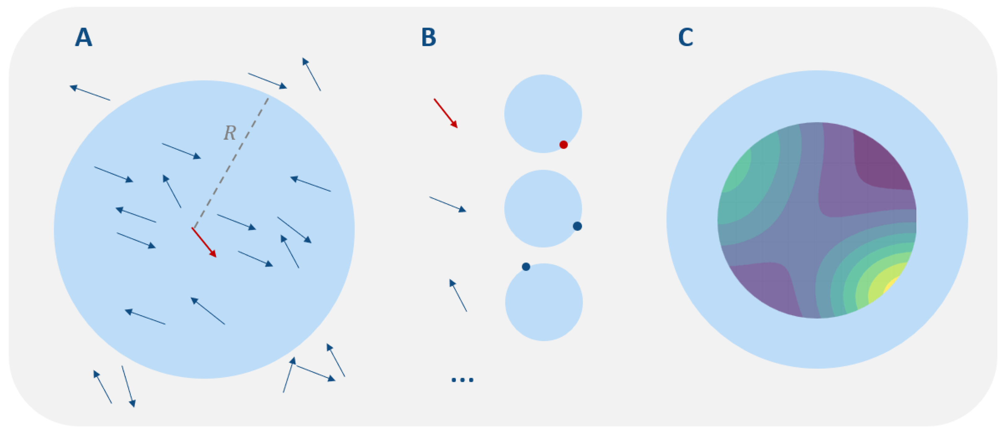
Spatial neighbourhood and directional encoding for KDE. (A) For a given radius , each sampled point (red arrow) defines a spatial neighbourhood (light-blue disc); neighbouring headings are shown as blue arrows. (B) Each heading is mapped to the unit circle by its sine and cosine, producing a point on the circle. (C) These encoded heading points are then used to fit the kernel density estimator.
Figure 6.
Spatial neighbourhood and directional encoding for KDE. (A) For a given radius , each sampled point (red arrow) defines a spatial neighbourhood (light-blue disc); neighbouring headings are shown as blue arrows. (B) Each heading is mapped to the unit circle by its sine and cosine, producing a point on the circle. (C) These encoded heading points are then used to fit the kernel density estimator.
Figure 7.
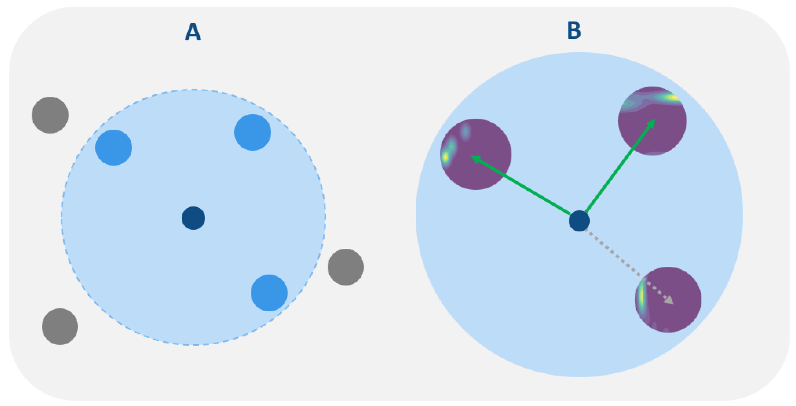
Edge criteria of xDAISTIN. (A) Neighbourhood criterion: only nodes within a radius (light blue area) are treated as candidate neighbours (light blue nodes) of a sampled node (dark blue); nodes outside (grey) are ignored. (B) Direction criterion: for each candidate neighbour, the potential edge direction is evaluated using the heading-based KDE. Edges are created only when this direction has probability above a threshold (solid green arrows); candidates that do not satisfy this threshold are discarded (dashed grey arrow).
Figure 7.
Edge criteria of xDAISTIN. (A) Neighbourhood criterion: only nodes within a radius (light blue area) are treated as candidate neighbours (light blue nodes) of a sampled node (dark blue); nodes outside (grey) are ignored. (B) Direction criterion: for each candidate neighbour, the potential edge direction is evaluated using the heading-based KDE. Edges are created only when this direction has probability above a threshold (solid green arrows); candidates that do not satisfy this threshold are discarded (dashed grey arrow).
Figure 8.
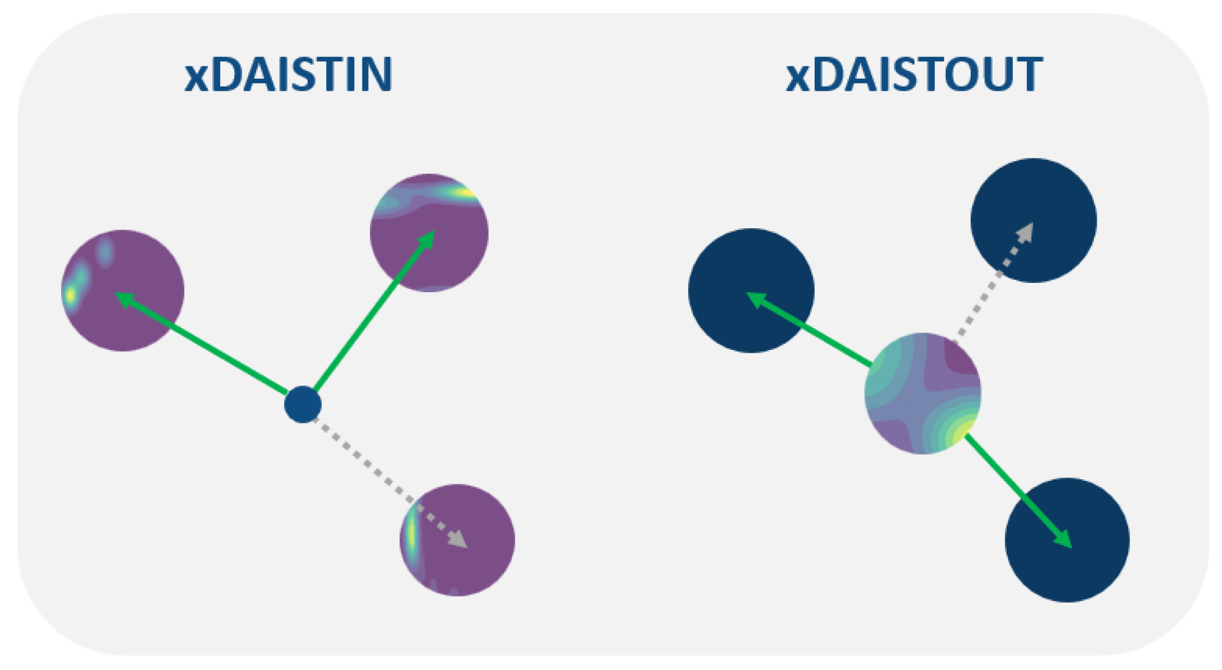
Comparison of the direction criterion used by xDAISTIN and xDAISTOUT. For a candidate directed edge from node A to node B, xDAISTIN evaluates the bearing using the circular heading density fitted at the destination node B, whereas xDAISTOUT evaluates the same bearing using the circular heading density fitted at the source node A. Solid green arrows represent candidate edges whose directional compatibility is within the probability thresholds and are therefore accepted; dotted grey arrows represent candidate edges that did not meet the criterion.
Figure 8.
Comparison of the direction criterion used by xDAISTIN and xDAISTOUT. For a candidate directed edge from node A to node B, xDAISTIN evaluates the bearing using the circular heading density fitted at the destination node B, whereas xDAISTOUT evaluates the same bearing using the circular heading density fitted at the source node A. Solid green arrows represent candidate edges whose directional compatibility is within the probability thresholds and are therefore accepted; dotted grey arrows represent candidate edges that did not meet the criterion.
Figure 9.
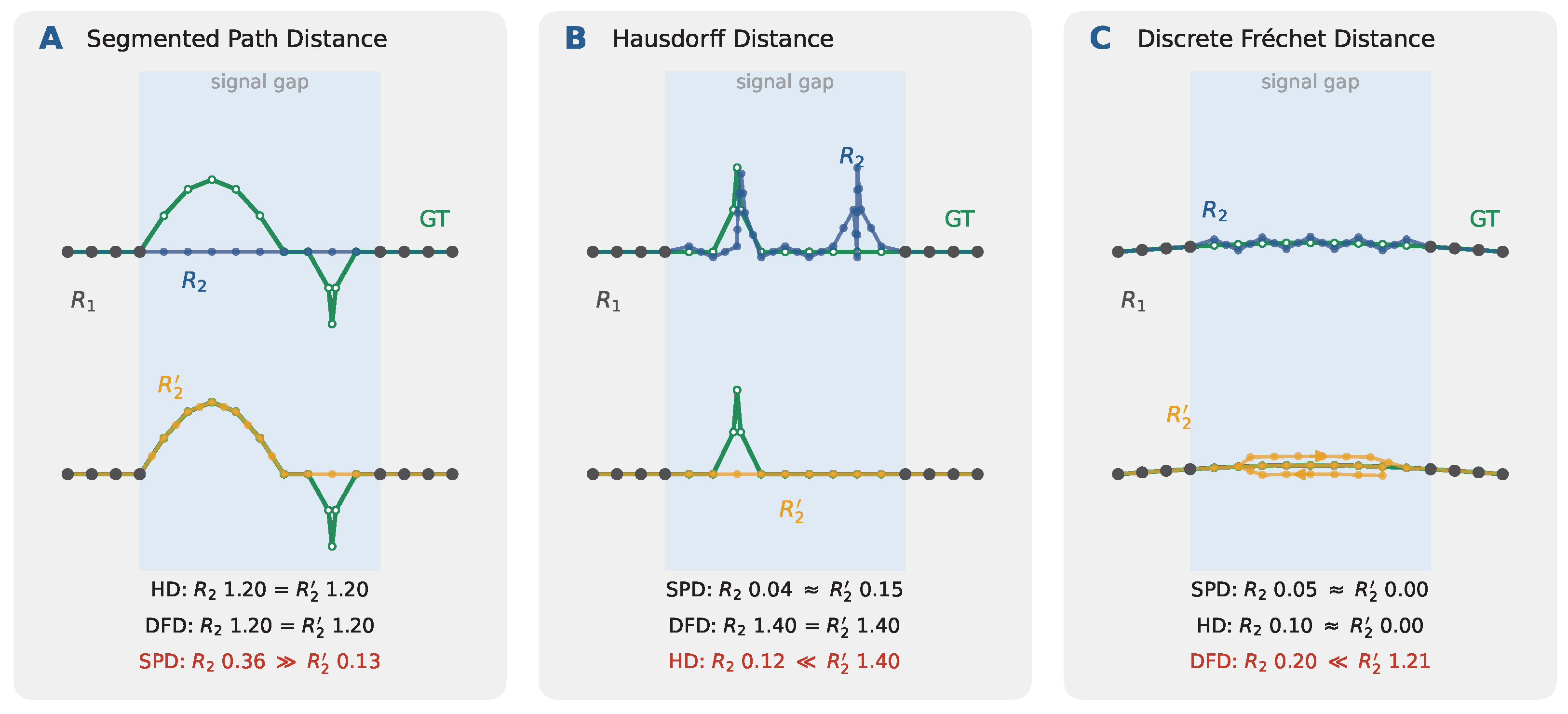
Evaluation metrics for trajectory reconstruction. Each panel shows the complete ground truth trajectory (GT, green), the sparse trajectory obtained by removing the observations inside the shaded signal gap, and two candidate interpolations of the gap, (blue, top row) and (orange, bottom row). Dots denote trajectory points, and red text highlights the metric illustrated in the corresponding panel. (A) Segmented Path Distance (SPD): an example in which SPD distinguishes between the two reconstructions, while HD and DFD assign them equal values. (B) Hausdorff Distance (HD): an example illustrating the sensitivity of HD to a large local deviation (green peak). (C) Discrete Fréchet Distance (DFD): an example in which a longer reconstruction is only penalized by DFD.
Figure 9.
Evaluation metrics for trajectory reconstruction. Each panel shows the complete ground truth trajectory (GT, green), the sparse trajectory obtained by removing the observations inside the shaded signal gap, and two candidate interpolations of the gap, (blue, top row) and (orange, bottom row). Dots denote trajectory points, and red text highlights the metric illustrated in the corresponding panel. (A) Segmented Path Distance (SPD): an example in which SPD distinguishes between the two reconstructions, while HD and DFD assign them equal values. (B) Hausdorff Distance (HD): an example illustrating the sensitivity of HD to a large local deviation (green peak). (C) Discrete Fréchet Distance (DFD): an example in which a longer reconstruction is only penalized by DFD.
Figure 10.
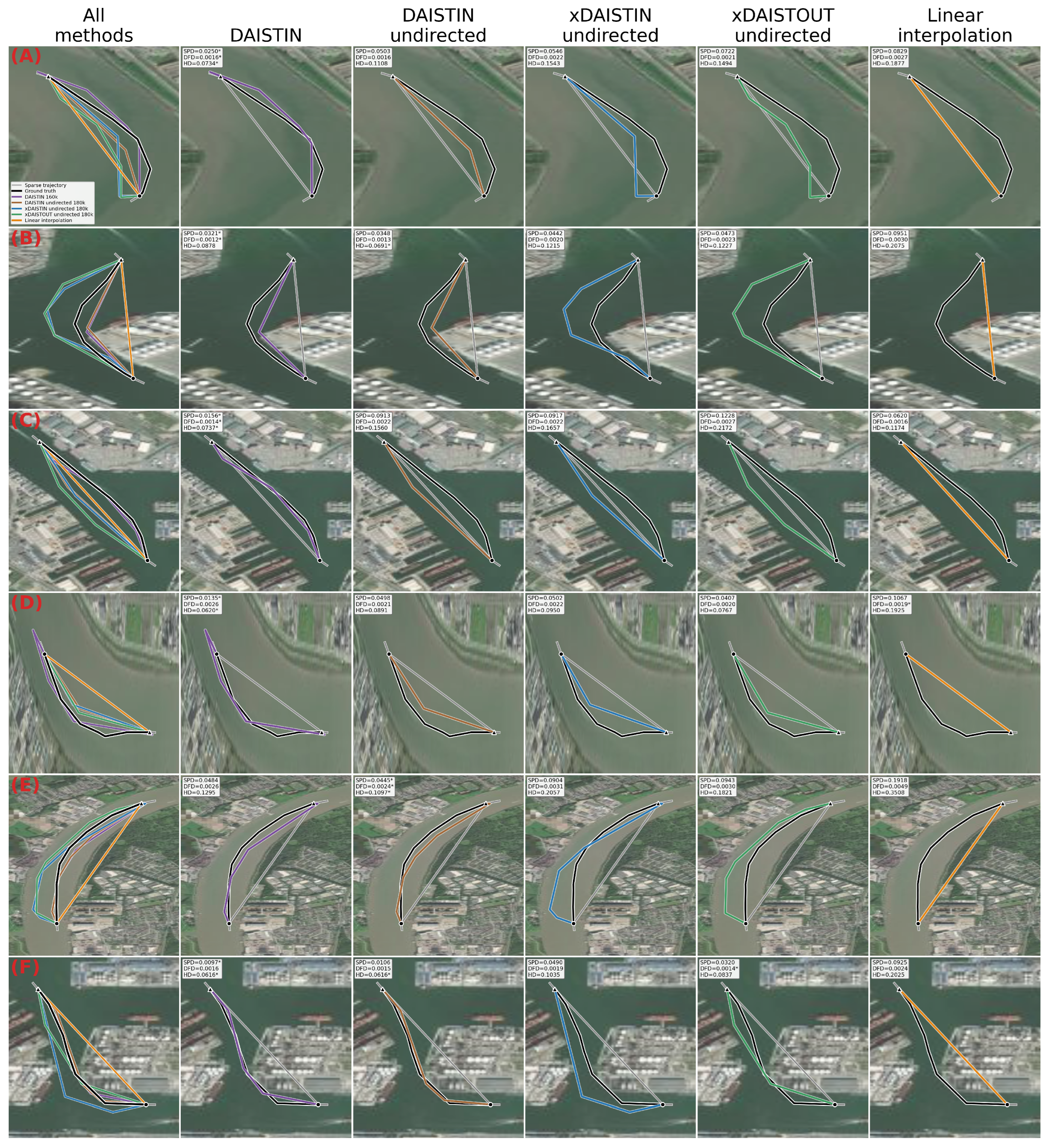
Qualitative examination of gap interpolation by DAISTIN variants. Selected cases (A–F) where gap interpolations are performed best by the DAISTIN variants according to SPD. Columns, in order, show the gap interpolation by all methods: DAISTIN (160 k), undirected DAISTIN (180 k), undirected xDAISTIN (180 k), undirected xDAISTOUT (180 k), and linear interpolation. Black trajectories denote ground truth and grey denotes the sparse observed trajectory. Asterisks denote the lowest reconstruction error for each metric within each case (row-wise).
Figure 10.
Qualitative examination of gap interpolation by DAISTIN variants. Selected cases (A–F) where gap interpolations are performed best by the DAISTIN variants according to SPD. Columns, in order, show the gap interpolation by all methods: DAISTIN (160 k), undirected DAISTIN (180 k), undirected xDAISTIN (180 k), undirected xDAISTOUT (180 k), and linear interpolation. Black trajectories denote ground truth and grey denotes the sparse observed trajectory. Asterisks denote the lowest reconstruction error for each metric within each case (row-wise).
Figure 11.
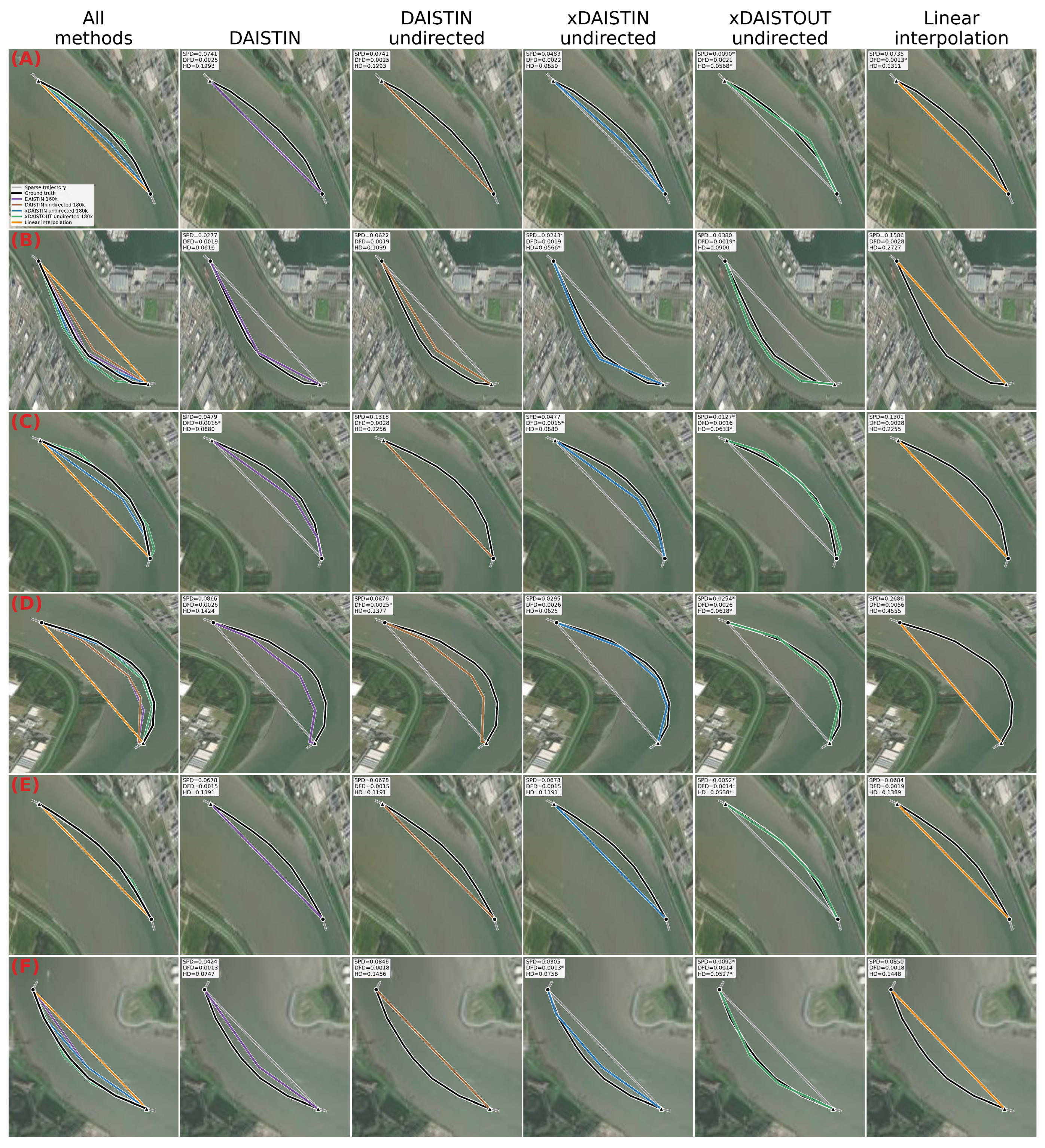
Qualitative examination of gap interpolation in corridors. Selected cases (A–F) where the gap is located in a corridor, with the xDAISTOUT undirected graph performing the best in most of them according to SPD. Columns, in order, show the gap interpolation by all methods: DAISTIN (160 k), undirected DAISTIN (180 k), undirected xDAISTIN (180 k), undirected xDAISTOUT (180 k), and linear interpolation. Black trajectories denote ground truth and grey denotes the sparse observed trajectory. Asterisks denote the lowest reconstruction error for each metric within each case (row-wise).
Figure 11.
Qualitative examination of gap interpolation in corridors. Selected cases (A–F) where the gap is located in a corridor, with the xDAISTOUT undirected graph performing the best in most of them according to SPD. Columns, in order, show the gap interpolation by all methods: DAISTIN (160 k), undirected DAISTIN (180 k), undirected xDAISTIN (180 k), undirected xDAISTOUT (180 k), and linear interpolation. Black trajectories denote ground truth and grey denotes the sparse observed trajectory. Asterisks denote the lowest reconstruction error for each metric within each case (row-wise).
Figure 12.
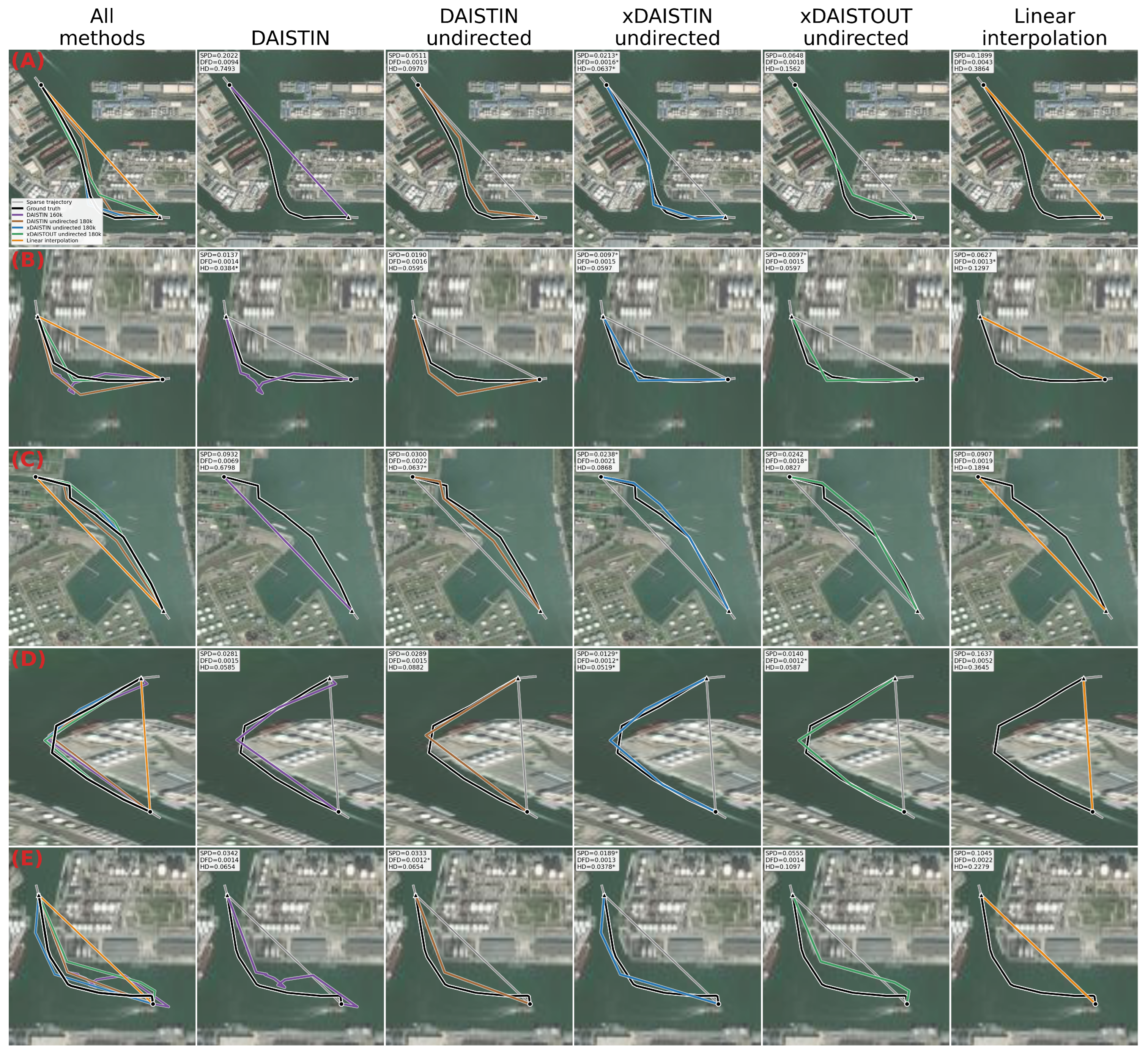
Qualitative examination of gap interpolation in confined inner-port waters. Selected cases (A–E) where gap interpolations are located in confined inner-port waters such as berths and terminals, with the xDAISTIN undirected graph performing the best in most of them according to SPD. Columns, in order, show the gap interpolation by all methods: DAISTIN (160 k), undirected DAISTIN (180 k), undirected xDAISTIN (180 k), undirected xDAISTOUT (180 k), and linear interpolation. Black trajectories denote ground truth and grey denotes the sparse observed trajectory. Asterisks denote the lowest reconstruction error for each metric within each case (row-wise).
Figure 12.
Qualitative examination of gap interpolation in confined inner-port waters. Selected cases (A–E) where gap interpolations are located in confined inner-port waters such as berths and terminals, with the xDAISTIN undirected graph performing the best in most of them according to SPD. Columns, in order, show the gap interpolation by all methods: DAISTIN (160 k), undirected DAISTIN (180 k), undirected xDAISTIN (180 k), undirected xDAISTOUT (180 k), and linear interpolation. Black trajectories denote ground truth and grey denotes the sparse observed trajectory. Asterisks denote the lowest reconstruction error for each metric within each case (row-wise).
Figure 13.
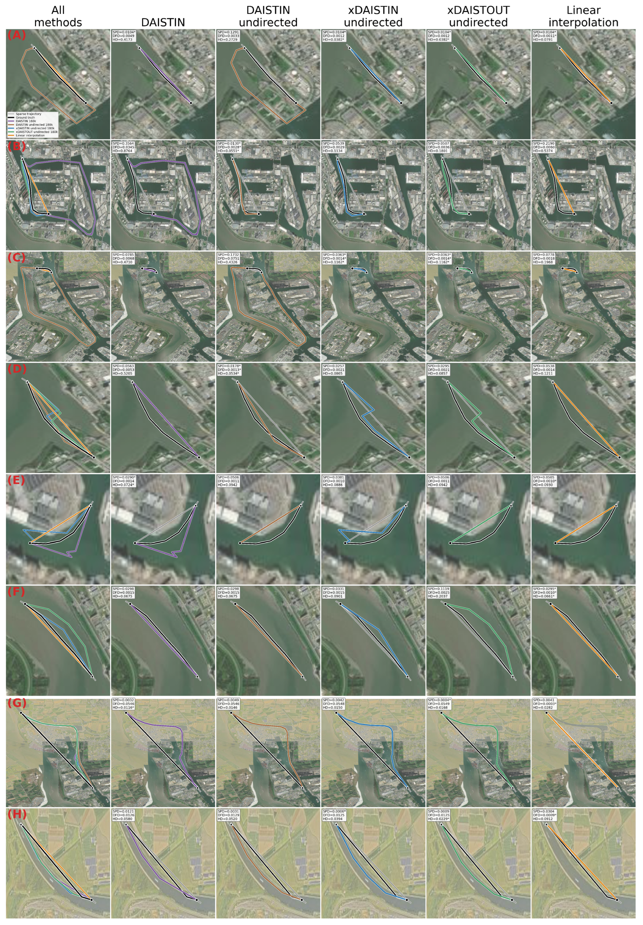
Reconstruction failures, artefacts, and incomplete ground truth cases. Selected cases illustrating directed and undirected DAISTIN artefacts (A–C), xDAISTIN and xDAISTOUT movement artefact (D), a gap where all methods struggle (E), a case favouring linear interpolation (F), and two cases with insufficiently detailed ground truth (G,H). Columns, in order, show the gap interpolation by all methods: DAISTIN (160 k), undirected DAISTIN (180 k), undirected xDAISTIN (180 k), undirected xDAISTOUT (180 k), and linear interpolation. Black trajectories denote ground truth and grey trajectories denote the sparse observed trajectory. Asterisks denote the lowest reconstruction error for each metric within each case (row-wise).
Figure 13.
Reconstruction failures, artefacts, and incomplete ground truth cases. Selected cases illustrating directed and undirected DAISTIN artefacts (A–C), xDAISTIN and xDAISTOUT movement artefact (D), a gap where all methods struggle (E), a case favouring linear interpolation (F), and two cases with insufficiently detailed ground truth (G,H). Columns, in order, show the gap interpolation by all methods: DAISTIN (160 k), undirected DAISTIN (180 k), undirected xDAISTIN (180 k), undirected xDAISTOUT (180 k), and linear interpolation. Black trajectories denote ground truth and grey trajectories denote the sparse observed trajectory. Asterisks denote the lowest reconstruction error for each metric within each case (row-wise).
Table 1.
Summary of the data set across processing steps. Numbers of AIS messages, unique vessels, extracted trips, and moving sub-trajectories retained after spatial restriction and cleaning, preprocessing, trip-level training/test partitioning, and the introduction of gaps in the test set. Data were collected via AISStream.io between 31 December 2023 and 24 January 2024. “–” denotes not applicable.
Table 1.
Summary of the data set across processing steps. Numbers of AIS messages, unique vessels, extracted trips, and moving sub-trajectories retained after spatial restriction and cleaning, preprocessing, trip-level training/test partitioning, and the introduction of gaps in the test set. Data were collected via AISStream.io between 31 December 2023 and 24 January 2024. “–” denotes not applicable.
| Data Set Stage | Messages | Vessels | Trips | Sub-Trajectories |
|---|
| Collected (raw) | 5,478,552 | 2654 | – | – |
| Spatially restricted and cleaned | 5,462,834 | 2553 | – | – |
| Preprocessed (moving sub-trajectories) | 956,995 | 2377 | 5488 | 36,748 |
| Training set (90% of trips) | 884,044 | † 2254 | 4939 | 34,124 |
| Test set (10% of trips) | 72,951 | † 478 | 549 | 2624 |
| Sparse test set (evaluation input) | 15,189 | 478 | 549 | 2624 |
Table 2.
Hyperparameter and evaluation-setting values. Final hyperparameter, implementation, and evaluation-setting values used in the reported experiments. The table uses “–” when a symbol is not specified for a parameter in the manuscript, and the superscript asterisk in denotes the target, rather than the actual, number of sampled graph nodes.
Table 2.
Hyperparameter and evaluation-setting values. Final hyperparameter, implementation, and evaluation-setting values used in the reported experiments. The table uses “–” when a symbol is not specified for a parameter in the manuscript, and the superscript asterisk in denotes the target, rather than the actual, number of sampled graph nodes.
| Parameter | Symbol | Value Used |
|---|
| Trip-segmentation time gap | | 6 h |
| Stopped-point speed threshold | | 1 knot |
| Minimum moving-sub-trajectory length | | 3 AIS data points |
| Training/test split ratio | – | |
| Hold-out split random seed | – | 50 |
| Gap-duration threshold distribution | | min, min |
| Target number of sampled graph nodes | | |
| Number of AND quantile groups | Q | 20 |
| Geometric-sampling ratio | | |
| AND neighbourhood radius | | 25 m |
| Heading-neighbourhood radius | | 25 m |
| KDE kernel | – | Gaussian |
| KDE bandwidth | – | |
| Minimum neighbouring headings for KDE fitting | – | 2 |
| Angular-window integration samples | – | 100 |
| Full-circle normalization samples | – | 720 |
| Candidate-edge radius | | 50 m |
| Angular half-window | | |
| Directional-probability threshold | | |
| Minimum speed used in travel-distance bound | – | 1 knot |
| Douglas–Peucker tolerance | – | |
| Interpolation trigger | – | 3 min |
| Post-processing densification threshold | – | 100 m |
Table 3.
Percentage of interpolated gaps across methods and number of nodes. Comparison of interpolation completion rate across all DAISTIN, xDAISTIN, and xDAISTOUT variants with varying number of graph nodes. Bold indicates the highest interpolation completion rate for a given number of nodes.
Table 3.
Percentage of interpolated gaps across methods and number of nodes. Comparison of interpolation completion rate across all DAISTIN, xDAISTIN, and xDAISTOUT variants with varying number of graph nodes. Bold indicates the highest interpolation completion rate for a given number of nodes.
| | Number of Nodes |
|---|
| Method | 100 k | 120 k | 140 k | 160 k | 180 k |
|---|
| DAISTIN | 48.48% | 63.45% | 75.98% | 80.62% | 84.61% |
| DAISTIN undirected | 72.35% | 78.94% | 85.46% | 89.36% | 91.23% |
| xDAISTIN | 88.02% | 90.83% | 92.81% | 94.91% | 96.42% |
| xDAISTIN undirected | 91.56% | 93.35% | 95.79% | 97.60% | 99.12% |
| xDAISTIN shortest | 91.36% | 94.03% | 95.39% | 95.72% | 97.46% |
| xDAISTIN undirected and shortest | 92.92% | 95.75% | 97.55% | 97.64% | 99.13% |
| xDAISTOUT | 65.75% | 72.52% | 78.44% | 82.40% | 85.17% |
| xDAISTOUT undirected | 91.56% | 93.20% | 95.55% | 97.43% | 97.80% |
| xDAISTOUT shortest | 72.12% | 76.45% | 81.12% | 85.87% | 89.08% |
| xDAISTOUT undirected and shortest | 92.89% | 95.48% | 97.33% | 97.43% | 97.80% |
Table 4.
Summary of evaluation of DAISTIN variations. Comparison of the original DAISTIN and the undirected variant across different graph sizes using SPD, HD, and DFD means. Matching coloured asterisks indicate non-significant differences between variants at the same graph size, whereas matching coloured crosses indicate non-significant differences between graph sizes for the same variant (). Bold indicates the best performance under a metric for a given number of nodes (column-wise).
Table 4.
Summary of evaluation of DAISTIN variations. Comparison of the original DAISTIN and the undirected variant across different graph sizes using SPD, HD, and DFD means. Matching coloured asterisks indicate non-significant differences between variants at the same graph size, whereas matching coloured crosses indicate non-significant differences between graph sizes for the same variant (). Bold indicates the best performance under a metric for a given number of nodes (column-wise).
| Metric | Variation | 100 k | 120 k | 140 k | 160 k | 180 k |
|---|
| SPD | Original | 0.0364 | 0.0344 | 0.0320 | 0.0311 | 0.0296 * |
| Undirected | 0.0339 | 0.0321 | +0.0307 | +0.0303 | +0.0302 * |
| Baseline (linear) | 0.0350 | 0.0350 | 0.0350 | 0.0350 | 0.0350 |
| DFD | Original | +0.0056 | +0.0056 | 0.0054 | 0.0052 * | 0.0047 |
| Undirected | +0.0049 | +0.0048 | 0.0044 | +0.0049 * | 0.0055 |
| Baseline (linear) | 0.0491 | 0.0491 | 0.0491 | 0.0491 | 0.0491 |
| HD | Original | 0.4348 | 0.3647 | 0.3030 | 0.2767 | 0.2402 |
| Undirected | 0.3222 | 0.2776 | 0.2332 | 0.2020 | 0.1919 |
| Baseline (linear) | 0.3070 | 0.3070 | 0.3070 | 0.3070 | 0.3070 |
Table 5.
Summary of evaluation of xDAISTIN variations. Comparison of the xDAISTIN graph variations across different graph sizes using SPD, HD, and DFD means. Matching coloured asterisks indicate non-significant differences between variants at the same graph size, whereas matching coloured crosses indicate non-significant differences between graph sizes for the same variant (). Bold indicates the best performance under a metric for a given number of nodes (column-wise).
Table 5.
Summary of evaluation of xDAISTIN variations. Comparison of the xDAISTIN graph variations across different graph sizes using SPD, HD, and DFD means. Matching coloured asterisks indicate non-significant differences between variants at the same graph size, whereas matching coloured crosses indicate non-significant differences between graph sizes for the same variant (). Bold indicates the best performance under a metric for a given number of nodes (column-wise).
| Metric | Variation | 100 k | 120 k | 140 k | 160 k | 180 k |
|---|
| SPD | Original | 0.0325 * | 0.0310 | 0.0298 | 0.0291 ** | 0.0286 ** |
| Undirected | 0.0304 | 0.0292 | 0.0274 | 0.0264 | 0.0258 |
| Shortest | 0.0345 | 0.0327 * | 0.0319 | 0.0290 * | 0.0288 * |
| Undirected and shortest | +0.0326 * | +0.0325 * | 0.0312 | 0.0285 * | 0.0282 * |
| Baseline (linear) | 0.0350 | 0.0350 | 0.0350 | 0.0350 | 0.0350 |
| DFD | Original | 0.0041 | 0.0039 | 0.0038 | 0.0037 | 0.0035 |
| Undirected | 0.0038 | 0.0037 | 0.0036 | 0.0034 | 0.0031 * |
| Shortest | +0.0075 | 0.0080 | +0.0078 | 0.0033 | 0.0031 ** |
| Undirected and shortest | 0.0068 | 0.0081 | 0.0079 | 0.0034 | 0.0031 * |
| Baseline (linear) | 0.0491 | 0.0491 | 0.0491 | 0.0491 | 0.0491 |
| HD | Original | 0.2418 | 0.2194 | 0.2095 | 0.1864 | 0.1729 |
| Undirected | 0.1921 * | 0.1811 | 0.1684 | 0.1476 | 0.1228 |
| Shortest | 0.2220 | 0.1992 | 0.1934 | 0.1737 | 0.1585 |
| Undirected and shortest | 0.1911 * | 0.1774 | 0.1708 | 0.1537 | 0.1303 |
| Baseline (linear) | 0.3070 | 0.3070 | 0.3070 | 0.3070 | 0.3070 |
Table 6.
Summary of evaluation of xDAISTOUT. Comparison of the xDAISTOUT graph variations across different graph sizes using SPD, HD, and DFD means. Matching coloured asterisks indicate non-significant differences between variants at the same graph size, whereas matching coloured crosses indicate non-significant differences between graph sizes for the same variant (). Bold indicates the best performance under a metric for a given number of nodes (column-wise).
Table 6.
Summary of evaluation of xDAISTOUT. Comparison of the xDAISTOUT graph variations across different graph sizes using SPD, HD, and DFD means. Matching coloured asterisks indicate non-significant differences between variants at the same graph size, whereas matching coloured crosses indicate non-significant differences between graph sizes for the same variant (). Bold indicates the best performance under a metric for a given number of nodes (column-wise).
| Metric | Variation | 100 k | 120 k | 140 k | 160 k | 180 k |
|---|
| SPD | Original | 0.0385 | 0.0370 | 0.0356 | 0.0347 | 0.0336 |
| Undirected | 0.0318 | 0.0308 | 0.0292 | 0.0284 * | 0.0278 |
| Shortest | 0.0368 | 0.0352 | 0.0336 | +0.0326 | +0.0327 |
| Undirected and shortest | +0.0326 | +0.0325 | 0.0313 | 0.0286 * | 0.0285 |
| Baseline (linear) | 0.0350 | 0.0350 | 0.0350 | 0.0350 | 0.0350 |
| DFD | Original | 0.0050 | 0.0048 | 0.0046 | 0.0044 | 0.0042 |
| Undirected | 0.0038 | 0.0038 | 0.0036 | 0.0034 | 0.0034 |
| Shortest | 0.0046 | +0.0044 | +0.0043 | +0.0040 | +0.0040 |
| Undirected and shortest | 0.0068 | 0.0081 | 0.0079 | 0.0034 | 0.0034 |
| Baseline (linear) | 0.0491 | 0.0491 | 0.0491 | 0.0491 | 0.0491 |
| HD | Original | 0.3924 | 0.3647 | 0.3313 | 0.2899 | 0.2630 |
| Undirected | 0.1937 | 0.1843 | 0.1739 * | 0.1533 | 0.1498 |
| Shortest | 0.3531 | 0.3326 | 0.3036 | 0.2576 | 0.2264 |
| Undirected and shortest | 0.1913 | 0.1786 | 0.1726 * | 0.1555 | 0.1538 |
| Baseline (linear) | 0.3070 | 0.3070 | 0.3070 | 0.3070 | 0.3070 |
Table 7.
Summary of selected graph configurations. Comparison of selected DAISTIN, xDAISTIN, and xDAISTOUT configurations using SPD, DFD, and HD means. Matching coloured crosses indicate pairs of configurations with no statistically significant difference for the corresponding metric (). Bold values indicate the lowest mean error for each metric.
Table 7.
Summary of selected graph configurations. Comparison of selected DAISTIN, xDAISTIN, and xDAISTOUT configurations using SPD, DFD, and HD means. Matching coloured crosses indicate pairs of configurations with no statistically significant difference for the corresponding metric (). Bold values indicate the lowest mean error for each metric.
| Metric | DAISTIN
Directed, 160 k | DAISTIN
Undirected, 180 k | xDAISTIN
Undirected, 180 k | xDAISTOUT
Undirected, 180 k |
|---|
| SPD | +0.0311 | +0.0302 | 0.0258 | 0.0278 |
| DFD | +0.0052 | +0.0055 | 0.0031 | 0.0034 |
| HD | 0.2767 | 0.1919 | 0.1228 | 0.1498 |
Table 8.
Offline graph construction runtime. Directed build time denotes full graph construction from the loaded sampled nodes for DAISTIN, xDAISTIN, and xDAISTOUT. Undirected build time denotes the additional time required to derive the undirected graph from the already constructed directed graph.
Table 8.
Offline graph construction runtime. Directed build time denotes full graph construction from the loaded sampled nodes for DAISTIN, xDAISTIN, and xDAISTOUT. Undirected build time denotes the additional time required to derive the undirected graph from the already constructed directed graph.
| Graph Family | Nodes | Directed Build | Undirected Build |
|---|
| | | Time (s) | Time (s) |
|---|
| DAISTIN | 100 k | 18.02 | 2.07 |
| DAISTIN | 180 k | 47.65 | 6.28 |
| xDAISTIN | 100 k | 575.51 | 10.90 |
| xDAISTIN | 180 k | 2477.60 | 42.78 |
| xDAISTOUT | 100 k | 578.24 | 8.76 |
| xDAISTOUT | 180 k | 2540.86 | 38.69 |
Table 9.
Online interpolation runtime for the main graph-based methods. Mean, median, standard deviation (Std.), and max times are computed at the gap-level over a random sample of 1000 gaps.
Table 9.
Online interpolation runtime for the main graph-based methods. Mean, median, standard deviation (Std.), and max times are computed at the gap-level over a random sample of 1000 gaps.
| Method | Nodes | Mean Time (s) | Median Time (s) | Std. Time (s) | Max Time (s) |
|---|
| DAISTIN | 100 k | 0.168 | 0.156 | 0.034 | 0.353 |
| DAISTIN | 180 k | 0.342 | 0.316 | 0.101 | 1.736 |
| DAISTIN undirected | 100 k | 0.187 | 0.171 | 0.051 | 0.492 |
| DAISTIN undirected | 180 k | 0.392 | 0.343 | 0.196 | 2.880 |
| xDAISTIN | 100 k | 0.540 | 0.424 | 0.361 | 4.413 |
| xDAISTIN | 180 k | 1.333 | 0.968 | 1.070 | 13.341 |
| xDAISTIN undirected | 100 k | 0.660 | 0.532 | 0.437 | 4.713 |
| xDAISTIN undirected | 180 k | 1.923 | 1.476 | 1.463 | 13.196 |
| xDAISTOUT | 100 k | 0.399 | 0.351 | 0.178 | 1.505 |
| xDAISTOUT | 180 k | 1.041 | 0.820 | 0.669 | 5.289 |
| xDAISTOUT undirected | 100 k | 0.662 | 0.535 | 0.448 | 4.844 |
| xDAISTOUT undirected | 180 k | 1.814 | 1.431 | 1.310 | 11.186 |