Early-Fusion Two-Channel ECG Scalograms and Transfer Learning for Record-Level Classification of Arrhythmia, Congestive Heart Failure and Normal Sinus Rhythm

Abstract

Automatic electrocardiogram (ECG) classification using deep learning is sensitive to data leakage, class imbalance and the way multi-segment decisions are aggregated at record level. This study presents a two-channel time–frequency early-fusion pipeline for classifying ECG recordings into arrhythmia (ARR), congestive heart failure (CHF) and normal sinus rhythm (NSR). The curated PhysioNet-derived ECGData dataset was used, comprising 81 reconstructed two-channel records: 48 ARR, 15 CHF and 18 NSR. Each 512 s ECG record, sampled at 128 Hz, was segmented into 10 s segments with 50% overlap. Continuous wavelet transform scalograms were generated for both ECG channels and horizontally fused into a single image representation for transfer learning with GoogLeNet. Signal-domain augmentation and class-weighted training were applied to improve robustness to small recording variations and class imbalance. To reduce leakage from overlapping segments, all segments from the same record were kept within the same fold during five-fold record-level cross-validation. Record-level predictions were obtained by averaging posterior probabilities across all segments from each record. The proposed early-fusion model achieved 94.83% mean segment-level accuracy and 98.77% aggregate record-level accuracy, correctly classifying 80 of 81 records. Under the same folds and training configuration, single-channel baselines achieved 75.31% and 87.65% aggregate record-level accuracy, indicating that two-channel early fusion improved classification reliability over single-channel ECG modelling. The only record-level error was a CHF recording classified as ARR. Although the results are promising, the CHF class contained only 15 records and the diagnostic classes originated from different source databases; therefore, further validation on larger, clinically verified multi-lead ECG datasets is required.

1. Introduction

Electrocardiography (ECG) remains one of the most widely used non-invasive tools for cardiac assessment because it is inexpensive, fast to acquire and rich in diagnostic information. The signal reflects the heart’s electrical activity and can support the detection of rhythm disturbances, conduction abnormalities, ischaemic change, structural disease, and broader markers of cardiac dysfunction [1]. Automated ECG interpretation is attractive for routine screening, long-duration monitoring, telemedicine, wearable sensing and decision support, particularly when large numbers of ECG segments must be reviewed. In this context, machine learning and deep learning methods can complement clinical expertise by identifying repeatable signal patterns across rhythm, morphology and time–frequency structure.

Deep learning has shifted ECG analysis from manually engineered features towards learned representations. One route uses one-dimensional convolutional or recurrent models directly on the waveform; another converts the signal into a two-dimensional representation, such as a continuous wavelet transform (CWT) scalogram, that can be processed using mature computer-vision architectures [2,3,4,5]. Transfer learning is especially attractive when the number of independent physiological recordings is small, because a pretrained network can provide a strong feature hierarchy that is fine-tuned for the target domain rather than trained from scratch [2,3,4].

However, high reported accuracy in ECG studies can be difficult to interpret. This is because the number of training images may be much larger than the number of independent recordings when long ECG traces are divided into overlapping segments; if segments from the same recording appear in both training and validation sets, the model may recognise record-specific morphology or acquisition characteristics rather than generalisable diagnostic structure. Long recordings are often segmented into many overlapping segments, but segments originating from the same record are strongly correlated. If training and validation sets are split at the segment level rather than the record or patient level, performance can be inflated through data leakage. The same concern is visible in recent biosignal work. Wosiak et al. showed that temporal segment shift and overlap can materially affect machine learning results and stressed the need for transparent reporting of segment length, shift and subject-wise evaluation [6]. Similarly, Grieger et al. emphasised data efficiency and small-subject regimes in EEG sleep staging, reinforcing the relevance of validation design when training data are limited [7].

A second challenge is channel utilisation. True multi-lead ECG contains complementary spatial views of cardiac electrical activity, and recent multi-lead ECG work has shown that cross-lead morphology and lead-specific information can be valuable for classification [8,9]. In the ECG data derivative used in this study, the two recordings from each source file were separated into individual rows during preprocessing. This study reconstructs those separated recordings into source-file two-channel records and evaluates whether early image fusion of their CWT scalograms improves classification relative to single-channel baselines under the same validation protocol.

The main contributions are as follows. First, the study reconstructs 81 two-channel records from a curated PhysioNet-derived ECG dataset and evaluates the model using record-level splits. Second, it proposes an interpretable early-fusion representation in which channel-wise CWT scalograms are concatenated with a narrow separator, allowing a standard pretrained CNN to learn joint lead information. Third, it combines physiologically constrained signal-domain augmentation with class-weighted transfer learning to address ARR/CHF/NSR class imbalance. Fourth, it reports both segment-level and record-level performance, including fold-to-fold variability, class-wise behaviour and an aggregate record-level confusion matrix. Fifth, a same-split single-channel ablation is added to isolate the contribution of the early-fusion representation.

2. Related Work and Methodological Positioning

Classical ECG classifiers generally combine denoising, beat detection, hand-crafted descriptors and shallow classifiers. Deep learning approaches can reduce dependence on manual feature design by learning discriminative morphology directly from waveforms or transformed images. CWT-based ECG image methods remain attractive because the transform localises signal content jointly in time and frequency, making the representation suitable for arrhythmia morphology that changes over short temporal intervals [5,10]. Wang et al. combined CWT scalograms with convolutional feature extraction and RR-interval information for arrhythmia classification, demonstrating that wavelet images can complement timing information [10]. Toma and Choi further showed that fusing temporal and scalogram-based branches can improve detection in imbalanced ECG arrhythmia tasks [11].

Transfer learning with pretrained image networks has also been widely adopted for ECG scalogram classification. The MathWorks reference workflow, from which the public ECGData.mat derivative is commonly used, demonstrates the conversion of PhysioNet ECG recordings into CWT RGB images and the adaptation of GoogLeNet or SqueezeNet to ARR, CHF and NSR labels [12]. This workflow is useful pedagogically, but its default image-level split does not fully address record-level dependence when segmentation and augmentation are introduced. The present study therefore treats record-level separation as a core methodological requirement.

Recent reviews emphasise that ECG deep learning studies are often difficult to compare directly because they use different datasets, segmentation units, diagnostic label definitions, preprocessing pipelines and data-splitting strategies [13,14]. For this reason, direct numerical comparison with published accuracy values should be interpreted cautiously and supported by transparent reporting of the experimental protocol. In the present study, the contribution of the two-channel early-fusion representation was therefore examined using a same-protocol single-channel baseline comparison. The channel 1, channel 2 and early-fusion models were trained and evaluated using the same record-level cross-validation folds, augmentation strategy, class weighting and GoogLeNet training configuration, allowing the effect of the two-channel time–frequency fusion representation to be assessed more directly.

The present work is positioned between specialised ECG architectures and lightweight transfer-learning workflows. It does not claim that GoogLeNet is optimal for ECG classification. In this manuscript, the classifier is the fine-tuned GoogLeNet network, whereas the wider algorithmic contribution is the complete processing and validation pipeline: CWT converts ECG segments into time–frequency images; two-channel early fusion defines how the two ECG-derived inputs are represented; record-level splitting defines how performance is estimated without segment reuse across training and validation; class balancing addresses the minority CHF class; and the segment-level versus record-level analysis shows how local segment predictions translate into recording-level decisions.

3. Materials and Methods

3.1. Dataset and Reconstruction of Two-Channel Records

All signal processing, CWT generation, transfer learning and evaluation were implemented in MATLAB R2024a (The MathWorks, Inc., Natick, MA, USA).

The experiments used ECGData.mat, a curated ECG dataset distributed through the MathWorks physionet_ECG_data repository and derived from three public PhysioNet [1] resources: the MIT-BIH Arrhythmia Database [15], the MIT-BIH Normal Sinus Rhythm Database [16] and the BIDMC Congestive Heart Failure Database [17]. In the distributed structure, ECGData.Data is a 162 × 65,536 matrix and ECGData.Labels contains diagnostic labels for ARR, CHF and NSR. The rows are sampled at 128 Hz, giving 512 s per row. The original source databases had different native sampling frequencies, but the distributed ECGData derivative had already been resampled to a common rate of 128 Hz before this study, as stated in the accompanying modified physionet data description. The MathWorks reference workflow treats these rows as individual ECG recordings for CWT-based image classification [18].

ECGData stores the separated channels in diagnostic/source blocks rather than as adjacent rows. The two-channel reconstruction therefore paired the first and second separated recordings within each block: ARR rows 1–48 with rows 49–96, CHF rows 97–111 with rows 112–126, and NSR rows 127–144 with rows 145–162. This reconstruction follows the accompanying modified physionet data file, which states that each source file consisted of two ECG recordings that were separated into two data records after scaling, resampling and truncation. The process produced 81 reconstructed two-channel records: 48 ARR, 15 CHF and 18 NSR. All subsequent splitting, augmentation and evaluation were controlled at the reconstructed-record level.

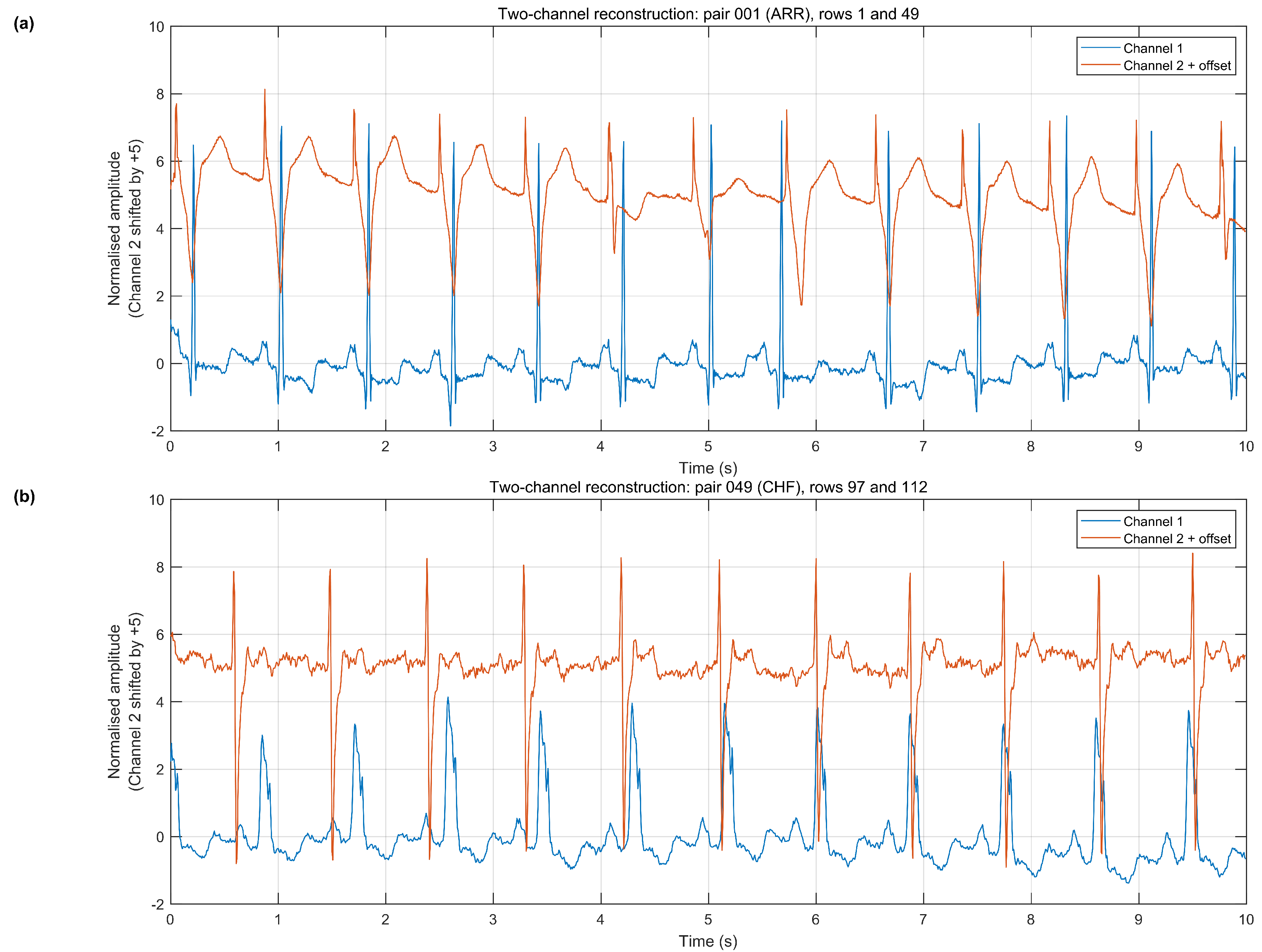
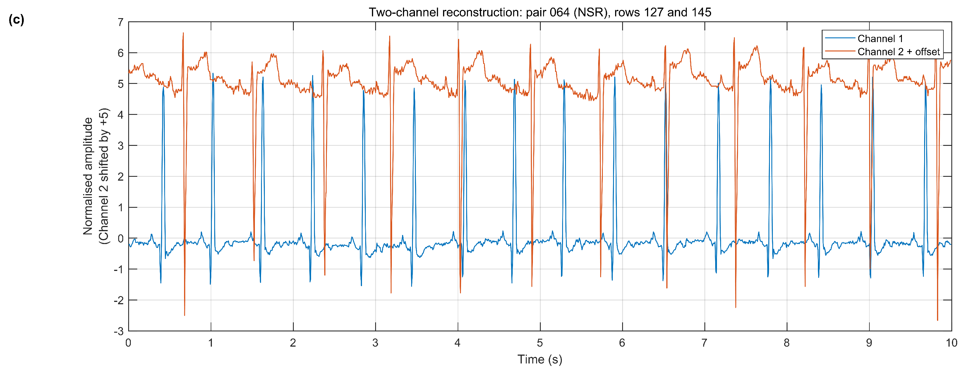
The reconstruction was checked programmatically by confirming label agreement, equal row length, the common 128 Hz sampling rate and preservation of each complete reconstructed record during splitting, augmentation and evaluation. Additional signal-level verification was performed using representative channel overlays to confirm corresponding beat sequences and QRS-complex regions. Because ECG channels may have different dominant QRS deflections, automated peak-to-peak offsets were not interpreted as direct lead delay; the verification was used to support the source-file reconstruction and to confirm that label agreement was not the only pairing criterion.

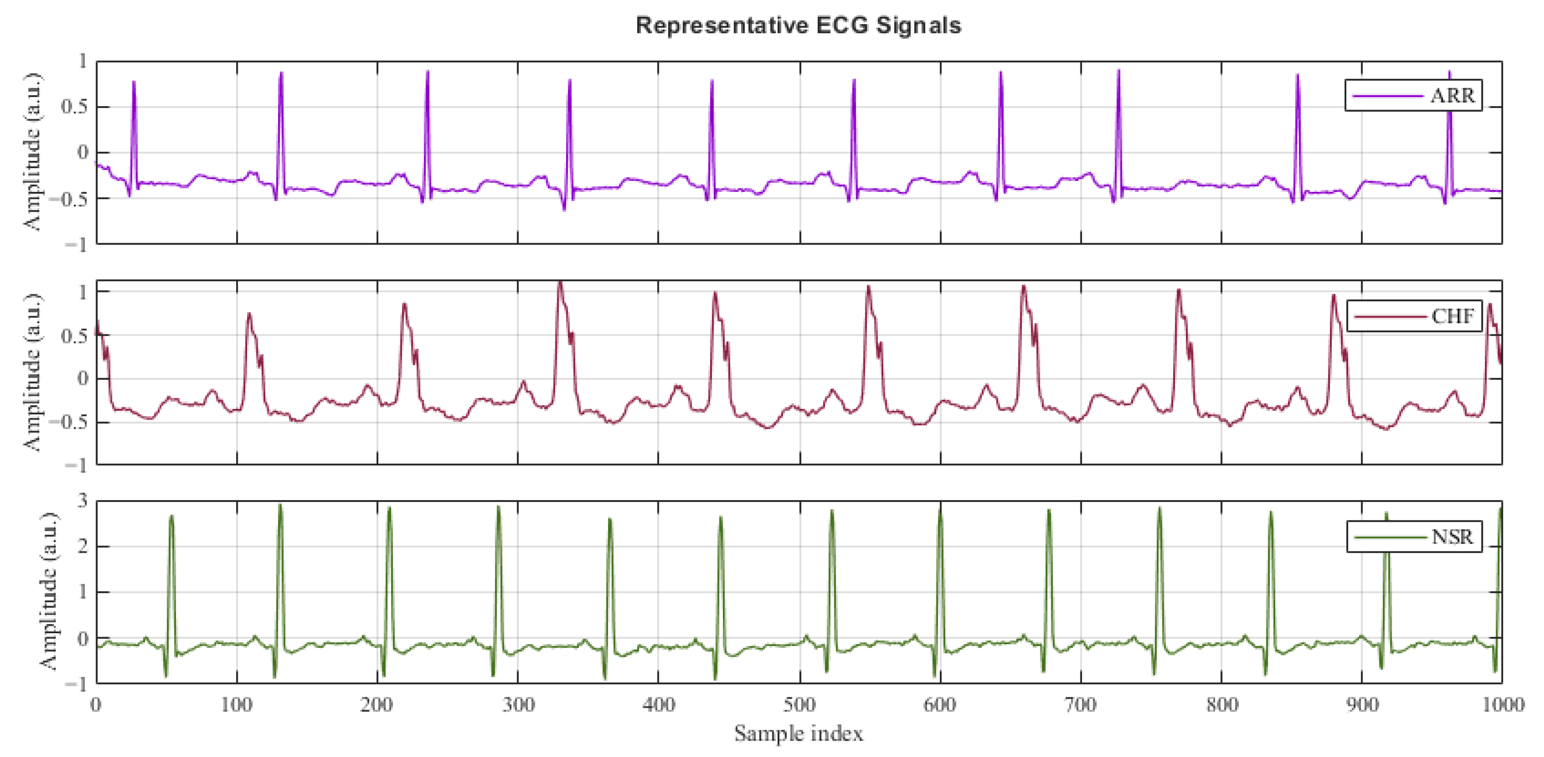
The class composition and reconstruction rule are summarised in

Table 1. Class composition and two-channel reconstruction rule.

Class	Source Database	Channel 1 Rows	Channel 2 Rows	Two-Channel Records	Share
ARR	MIT-BIH Arrhythmia	1–48	49–96	48	59.26%
CHF	BIDMC Congestive Heart Failure	97–111	112–126	15	18.52%
NSR	MIT-BIH Normal Sinus Rhythm	127–144	145–162	18	22.22%
Total	Three PhysioNet-derived sources	81 rows	81 rows	81	100.00%

, and representative class excerpts are shown in Figure 1.

3.2. Leakage-Aware Segmentation and Cross-Validation

Each channel in a reconstructed two-channel record was segmented using a 10 s segment with 50% overlap. At 128 Hz, this corresponds to 1280 samples per segment and a step size of 640 samples. The 10 s duration was selected to provide more temporal context than a short beat-level representation while still generating enough training images for transfer learning.

To prevent data leakage, all segments generated from the same reconstructed two-channel record were kept within the same fold, where a fold denotes one complete training–validation partition used during cross-validation. In each fold, a reconstructed record was assigned either to the training subset or to the validation subset, but never to both. Data leakage here means an inflated validation estimate caused by highly correlated overlapping segments from the same source record appearing in both training and validation subsets. No augmented or non-augmented segment from a validation record was allowed to appear in the training subset. After a targeted development split was used for hyperparameter selection, the selected configuration was evaluated using five-fold record-level cross-validation, meaning that the reconstructed records were divided into five validation rounds and each record served as validation data once.

3.3. Signal Preprocessing, Signal-Domain Augmentation and Class Balancing

The distributed ECGData derivative had already been scaled using PhysioNet file information, resampled to 128 Hz and truncated to 65,536 samples. In this study, preprocessing before CWT image formation was intentionally conservative: non-finite values, if present, were replaced by the finite-segment median; the median was subtracted from each 10 s segment to remove DC offset; and no additional diagnostic band-pass filtering or automated artefact-rejection step was applied. Signal quality control was limited to checking finite values, common length, common sampling rate and consistent record-level allocation. Amplitude normalisation was applied after CWT by rescaling each scalogram magnitude to [0,1].

Class imbalance was addressed at the segment level but without moving any record across fold boundaries. Augmentation was applied only to training segments and only to minority classes. In the representative 64-record training folds, ARR contributed 3838 base segments, CHF 1212 and NSR 1414. Augmentation increased CHF and NSR to 3071 segments each, while ARR remained unchanged. This produced 9980 training segments in those folds. Class-weighted loss was also used to reduce the effect of remaining imbalance. Representative base, augmented and validation segment counts are listed in

Table 2. Representative segment counts before and after augmentation for a 64-record training fold.

Class	Base Training Segments	Augmented Segments Generated	Final Training Segments	Validation Segments
ARR	3838	0	3838	1010
CHF	1212	1859	3071	303
NSR	1414	1657	3071	404
Total	6464	3516	9980	1717

.

Augmentation was applied in the signal domain before scalogram generation. For each augmented fusion sample, the same transformation was applied to both channels to preserve inter-channel temporal alignment. The operators were gain jitter up to ±5%, temporal shift up to ±0.10 s, mild time warping up to ±3% with probability 0.30, baseline wander at 0.15–0.40 Hz with amplitude up to 4% of channel standard deviation and probability 0.60, and additive white noise with probability 0.85 and signal-to-noise ratio sampled from 24–34 dB. These values were selected as conservative nuisance perturbations rather than diagnostic transformations: gain jitter represents electrode-contact or amplitude-calibration variation; temporal shift represents segment-boundary uncertainty; baseline wander represents respiration, motion or electrode drift; and additive noise represents measurement contamination. The ±3% time-warp factor changes the local time scale only mildly and was included to improve robustness to small rate variation, while limiting the risk of unintentionally moving physiological features such as QRS or QT duration into clearly pathological ranges. They were designed to reduce sensitivity to small physiological and recording variations while avoiding unrealistic image transformations that could distort diagnostic morphology.

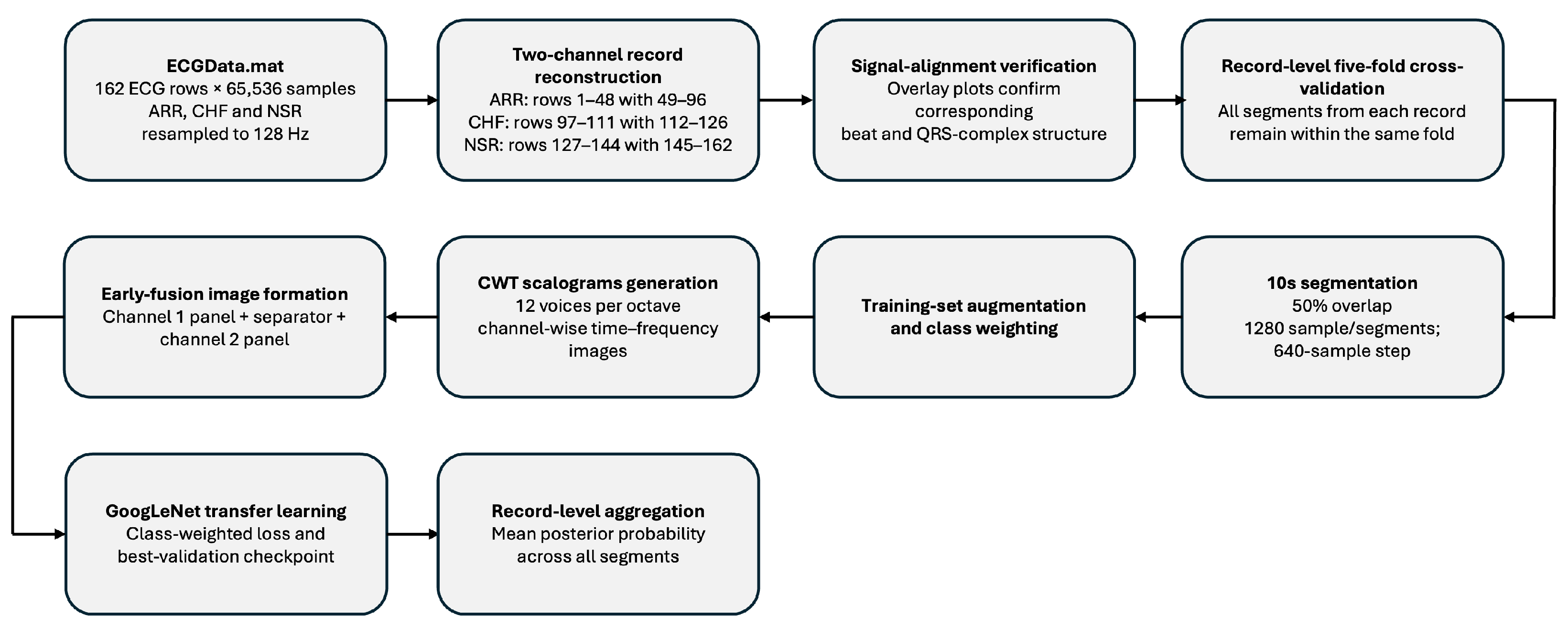
The complete processing sequence is summarised in Figure 2; bold text denotes each principal processing stage, whereas regular text gives its corresponding configuration or output.

Representative reconstructed two-channel ECG excerpts used to verify paired-channel correspondence are presented in Figure 3. Panels (a)–(c) show the first 10s at 128 Hz for ARR pair 001, CHF pair 049 and NSR pair 064, respectively.

3.4. Continuous Wavelet Transform and Early-Fusion Scalogram Construction

A CWT filter bank was generated for each 10 s segment using a sampling frequency of 128 Hz and 12 voices per octave. In wavelet terminology, an octave is a doubling of frequency, and voices per octave is the number of CWT scales or wavelet filters placed within each factor-of-two frequency interval. Thus, 12 voices per octave uses 12 logarithmically spaced wavelet filters between f and 2f, giving a slightly denser scale sampling than the MATLAB R2024a default of 10 [19]. This density was selected to provide a moderately fine time–frequency representation of the P-QRS-T complex without producing an unnecessarily large image representation for transfer learning. For a signal $x\left(t\right)$, the CWT can be written as

$${\mathrm{CWT}}_x(a,b)=\int x\left(t\right){\psi }_{a,b}^{*}\left(t\right)dt$$

(1)

where ${\mathrm{CWT}}_x(a,b)$ compares $x\left(t\right)$ with scaled and shifted versions of the mother wavelet $\psi \left(t\right)$; a denotes scale and b denotes time translation. The absolute coefficient magnitude forms the scalogram.

For each channel segment, the scalogram magnitude was normalised by its maximum coefficient magnitude and mapped to an RGB image following

$$S_N={\displaystyle \frac{|{\mathrm{CWT}}_x|}{max\left(\right|{\mathrm{CWT}}_x\left|\right)}}$$

(2)

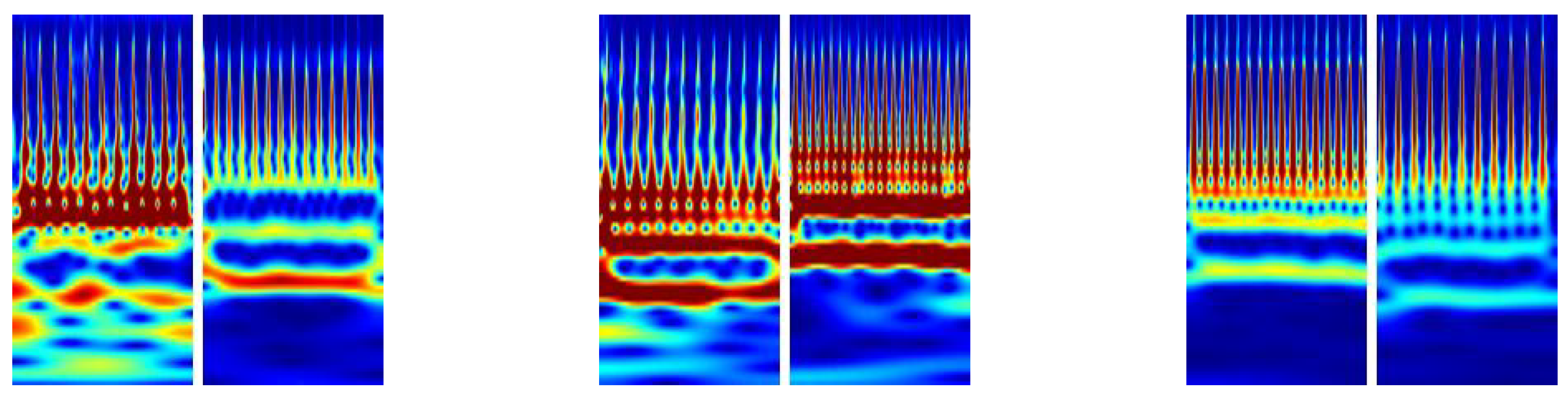
The implementation used a 224 × 224 × 3 GoogLeNet input canvas. For early fusion, the two channel-specific scalograms were converted using the same colormap and normalisation rule, resized to fit left and right panels, and concatenated horizontally with a narrow white separator. This horizontal integration preserves channel-specific morphology while allowing the CNN to learn cross-channel visual patterns from a single input image. The design intentionally avoids feature-level or decision-level fusion complexity while preserving complementary channel information. Examples of the resulting class-specific fused images are shown in Figure 4.

3.5. Transfer Learning with GoogLeNet

GoogLeNet was selected as the backbone because its Inception architecture provides a strong pretrained feature hierarchy with a more moderate parameter burden than very deep VGG-style models [2]. The original final layers were replaced by a dropout layer, a new three-class fully connected layer and a classification layer for ARR, CHF and NSR. The new fully connected layer used increased learning-rate factors for weights and bias to accelerate adaptation of the newly initialised parameters.

Training used best-validation checkpointing where supported by the MATLAB release. The returned model therefore corresponded to the best validation point observed during training rather than necessarily the last epoch. This is important in small-data transfer learning, where training accuracy can approach 100% before validation performance stabilises.

3.6. Hyperparameter Selection

A targeted four-trial search was performed on a development hold-out split in which complete paired units, rather than individual segments, were assigned to training or validation. The search varied initial learning rate, mini-batch size, dropout and L2 regularisation. Candidate settings were ranked using a pre-specified development score that intentionally favoured balanced class performance and CHF sensitivity rather than accuracy alone:

$$J=F_{1,\mathrm{macro}}^{\mathrm{seg}}+0.05R_{\mathrm{CHF}}+0.02F_{1,\mathrm{macro}}^{\mathrm{rec}}$$

(3)

This objective was a pragmatic model-selection score, not a proposed clinical utility function. Equation (3) is a linear scalarisation of three development-set criteria: segment-level macro F1 as the dominant term, CHF recall as a small minority-class sensitivity term, and record-level macro F1 as a small stability term. The coefficients 0.05 and 0.02 were deliberately small so that secondary criteria could break ties or penalise weak CHF behaviour without overriding the main macro F1 objective. Segment-level macro F1 was the dominant term because it gives equal weight to ARR, CHF and NSR. The CHF-recall term was included because CHF was the smallest class and false negatives are undesirable; the small coefficient limited this to a secondary influence. The record-level macro F1 term was also small because the development split contained few paired units, making record-level estimates useful but statistically coarse. The four candidate configurations and their development results are reported in

Table 3. Targeted hyperparameter search on the development hold-out split.

Trial	Initial LR	Mini- Batch	Dropout	L2	Val. Segment Macro F1	Val. CHF Recall	Objective
1	${10}^{-4}$	16	0.5	${10}^{-4}$	0.8821	0.6898	0.9366
2	$3\times {10}^{-4}$	16	0.6	${10}^{-4}$	0.9361	0.8449	0.9984
3	${10}^{-4}$	24	0.5	$5\times {10}^{-4}$	0.9293	0.8185	0.9902
4	$3\times {10}^{-4}$	24	0.6	$5\times {10}^{-4}$	0.8736	0.6370	0.9238

.

3.7. Evaluation Metrics and Record-Level Aggregation

Performance was quantified at two levels. At the segment level, each fused 10 s image was classified independently. Accuracy, precision, recall, specificity and F1-score were computed per class, with macro F1 and weighted F1 used as summary measures. Macro F1 gives equal weight to ARR, CHF and NSR, while weighted F1 accounts for support.

At record level, the softmax posterior probabilities from all segments belonging to the same reconstructed record were averaged. The final record label was assigned by maximum mean posterior probability:

$${\widehat{y}}_r=arg\underset{c}{max}\left({\displaystyle \frac{1}{N_r}}\sum _{i}p(c\mid x_i)\right)$$

(4)

where $N_r$ is the number of segments from record r. Thus, record-level aggregation used mean posterior evidence rather than majority voting; majority-vote counts were inspected only for error analysis. Record-level metrics were computed from out-of-fold validation records pooled across the five folds. Record-level aggregation is clinically meaningful because the diagnostic label belongs to the full recording, not to isolated overlapping segments.

4. Results

4.1. Five-Fold Cross-Validation Summary

Table 4. Five-fold segment-performance summary for the proposed two-channel early-fusion model.

Fold	Train Records	Val. Pairs	Val. Acc.	Val. Macro F1	Val. Weighted F1	Val. CHF Recall
1	64	17	0.8917	0.8613	0.8887	0.6700
2	64	17	0.9744	0.9669	0.9742	0.9076
3	64	17	0.9936	0.9936	0.9936	0.9967
4	66	15	0.9380	0.9293	0.9374	0.9142
5	66	15	0.9439	0.9326	0.9417	0.7624

reports fold-level segment performance for the two-channel early-fusion model using source-file reconstruction and fixed hyperparameters. Mean validation segment accuracy across the five folds was 94.83%, with a median of 94.39% and range 89.17–99.36%. Validation segment macro F1 averaged 0.9367 and weighted F1 averaged 0.9471.

Table 5. Five-fold record-performance summary.

Fold	Train Record Acc.	Val. Record Acc.	Val. Record Macro F1	Val. Record Weighted F1	Val. CHF Recall
1	1.0000	0.9412	0.9175	0.9367	0.6667
2	1.0000	1.0000	1.0000	1.0000	1.0000
3	1.0000	1.0000	1.0000	1.0000	1.0000
4	1.0000	1.0000	1.0000	1.0000	1.0000
5	1.0000	1.0000	1.0000	1.0000	1.0000

reports the corresponding record-level results. Four of the five folds achieved perfect record-level validation accuracy; fold 1 misclassified one of the three CHF validation records, yielding 94.12% record accuracy for that fold. Because record-level accuracy is bounded by 0 and 100% and the fold distribution is skewed, record-level performance is reported primarily as aggregate accuracy and median/range rather than as mean ± SD. The pooled out-of-fold record-level accuracy was 98.77% (80/81 records). The corresponding five-fold summary statistics are consolidated in

Table 6. Aggregate five-fold summary statistics.

Metric	Mean	Median	Min.	Max.
Train segment accuracy	0.9998	0.9999	0.9990	1.0000
Validation segment accuracy	0.9483	0.9439	0.8917	0.9936
Validation segment macro F1	0.9367	0.9326	0.8613	0.9936
Validation segment weighted F1	0.9471	0.9417	0.8887	0.9936
Validation record accuracy	0.9882	1.0000	0.9412	1.0000
Validation record macro F1	0.9835	1.0000	0.9175	1.0000
Validation record weighted F1	0.9873	1.0000	0.9367	1.0000
Validation CHF recall (segment)	0.8502	0.9076	0.6700	0.9967
Validation CHF recall (record)	0.9333	1.0000	0.6667	1.0000

, and the segment- and record-level validation accuracies are visualised in Figure 5.

4.2. Class-Wise Segment-Level Behaviour

Class-wise segment performance showed meaningful fold-to-fold variation. Across folds, mean segment-level F1 was 0.9598 for ARR, 0.8897 for CHF and 0.9607 for NSR. CHF remained the most variable class: its segment-level recall ranged from 0.6700 in fold 1 to 0.9967 in fold 3. This variability indicates that CHF examples were not uniformly difficult; rather, some fold compositions produced substantially more ambiguous CHF segments than others.

The strongest segment-level performance occurred in fold 3, where validation accuracy reached 99.36%. The weakest segment-level performance occurred in fold 1, where CHF recall was lowest and the only record-level error occurred. Importantly, record-level aggregation resolved most segment-level uncertainty, but not all of it: one CHF record whose mean probability was assigned to ARR remained misclassified. The fold-aggregated class-wise values are reported in

Table 7. Class-wise segment-level precision, recall and F1-score across five folds.

Class	Precision Mean ± SD	Recall Mean ± SD	F1 Mean ± SD	Total Validation Segments
ARR	0.9501 ± 0.0377	0.9701 ± 0.0312	0.9598 ± 0.0307	4848
CHF	0.9367 ± 0.0842	0.8502 ± 0.1314	0.8897 ± 0.1058	1515
NSR	0.9545 ± 0.0359	0.9698 ± 0.0640	0.9607 ± 0.0354	1818

, and their mean F1-scores with standard deviations are shown in Figure 6.

4.3. Aggregate Record-Level Confusion Matrix

Pooling the validation records across the five folds produced 81 out-of-fold record predictions. The aggregate record-level confusion matrix contained 80 correct predictions and one error. All 48 ARR records and all 18 NSR records were correctly classified. Fourteen of the 15 CHF records were correctly classified, while one CHF record was assigned to ARR. This gives a pooled record-level accuracy of 98.77%. For the minority CHF class, recall was 14/15 = 93.33%; the Wilson 95% confidence interval was 70.18–98.81%, reflecting the statistical instability caused by the small number of CHF records. The pooled confusion matrix is shown in Figure 7, with class-wise recall and Wilson intervals reported in

Table 8. Pooled aggregate record-level metrics and Wilson confidence intervals.

Class	Correct/Total	Recall	Wilson 95% CI
ARR	48/48	100.00%	92.59–100.00%
CHF	14/15	93.33%	70.18–98.81%
NSR	18/18	100.00%	82.41–100.00%

.

The only record-level fusion error was pair 62, a CHF record predicted as ARR. The record-level decision was based on the mean posterior probability across 101 segments. For this record, the mean posterior score was highest for ARR (0.7335), followed by NSR (0.2148) and CHF (0.0517). The segment-vote distribution was 83 ARR, 1 CHF and 17 NSR, indicating that the error reflected a consistent record-level representation rather than a small number of unstable segments.

4.4. Same-Split Single-Channel Ablation

To isolate the contribution of early fusion, two additional single-channel GoogLeNet baselines were trained and evaluated using the same reconstructed records, the same five record-level folds, the same augmentation policy, the same class-weighted loss and the same training configuration. The proposed early-fusion model achieved 98.77% aggregate record-level accuracy (80/81 records), compared with 75.31% for channel 1 and 87.65% for channel 2. At the segment level, mean validation accuracy was 94.83% for early fusion, 72.45% for channel 1 and 80.94% for channel 2. These results indicate that the performance gain is attributable to the two-channel representation under controlled validation, rather than to differences in splitting, augmentation or classifier configuration. The controlled comparison is summarised in

Table 9. Comparison of single-channel and two-channel early-fusion models using segment-level and aggregate record-level accuracy.

Model	Input	Mean Segment Acc.	Median Segment Acc.	Aggregate Record Acc.	Correct Records
Single-channel 1	Channel 1 CWT scalogram	72.45%	79.21%	75.31%	61/81
Single-channel 2	Channel 2 CWT scalogram	80.94%	90.62%	87.65%	71/81
Two-channel early fusion	Two fused CWT scalograms	94.83%	94.39%	98.77%	80/81

.

5. Discussion

5.1. Interpretation of the Main Findings

The five-fold results support the value of early fusion when two ECG recordings from the same source file are available. The proposed model achieved high record-level performance while maintaining a strict record-level split that prevented overlapping segments from the same reconstructed record appearing in both training and validation. The same-split ablation strengthens this conclusion: early fusion improved aggregate record-level accuracy by 23.46 percentage points relative to channel 1 and by 11.11 percentage points relative to the stronger channel 2 baseline. This suggests that the two-channel time–frequency image contains complementary information that is useful to the pretrained CNN.

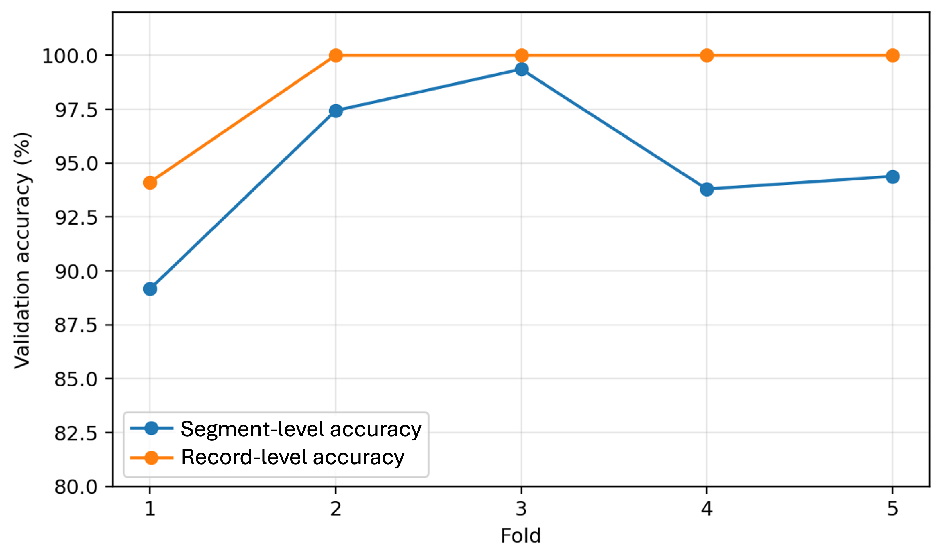
At the same time, the segment-level results reveal important residual uncertainty. Mean validation segment accuracy was high, but fold-to-fold variation was substantial. CHF recall at segment level was especially unstable, falling to 0.6700 in fold 1 and 0.7624 in fold 5. This pattern is clinically important: a model can produce a correct record-level decision while still being uncertain across many constituent segments. Reporting only record-level accuracy would therefore conceal segment-level ambiguity; reporting only segment-level performance would understate the stabilising effect of aggregation. The two views are complementary.

The observed gap between training and validation performance also requires caution. Training segment accuracy approached 100%, indicating that the augmented training set was almost perfectly fitted. Validation segment accuracy remained lower, suggesting useful generalisation but also clear overfitting risk. This is expected because the apparent number of images is much larger than the number of independent records. The study therefore supports record-level splitting as a minimum standard for this type of ECG-image workflow.

5.2. Why Early Fusion Is Useful but Not Sufficient

The early-fusion representation has practical advantages. It is transparent, easy to reproduce and compatible with standard pretrained image networks. Unlike simple channel averaging or single-lead selection, it preserves lead-specific time–frequency morphology. Unlike complex lead-attention architectures, it can be implemented with limited code and computational overhead. This makes it suitable for small datasets and for exploratory work where reproducibility matters.

The classification-stage inference time was similar across the early-fusion and single-channel models because all inputs were resized to the same GoogLeNet input dimensions. Across the five folds, mean validation inference time was 2.47 s for early fusion, compared with 2.50 s and 2.32 s for the channel 1 and channel 2 baselines. The main additional computational cost of early fusion is therefore expected during preprocessing, where two CWT scalograms must be generated instead of one; once the fused image is formed, CNN inference cost is comparable to the single-channel baselines.

However, early fusion is not a substitute for more principled lead modelling. A CNN receiving a dual-panel image must learn inter-lead relationships implicitly. It has no explicit representation of lead geometry, temporal synchrony or cardiac electrophysiology. Recent multi-lead ECG studies using lead generation, lead encoder attention and hierarchical feature extraction demonstrate that more specialised architectures may exploit cross-lead structure more effectively [8,9]. Future versions of the present pipeline could therefore compare early image fusion with feature-level lead attention, cross-lead transformers or multi-branch architectures.

5.3. Relationship to Prior Work

The proposed method builds on established ECG classification workflows that transform one-dimensional ECG signals into two-dimensional time–frequency images before applying transfer learning with pretrained convolutional neural networks. The MathWorks CWT-GoogLeNet reference workflow demonstrates this approach by converting individual ECG signals into RGB scalograms and fine-tuning GoogLeNet, reporting a validation accuracy of 93.75% [18]. The present study complements this external reference by adding same-split single-channel baselines using the identical record-level five-fold protocol.

First, rather than treating each ECG row as an isolated single-channel signal, the proposed method reconstructs two-channel records from the separated ECG recordings in each source file and performs early fusion of their CWT scalograms. Second, evaluation is performed at reconstructed-record level rather than by randomly splitting individual scalogram images. Third, the study reports both segment-level and record-level performance. Fourth, the same-split ablation shows that early fusion outperformed both single-channel baselines under the same validation protocol, supporting the specific contribution of the two-channel representation.

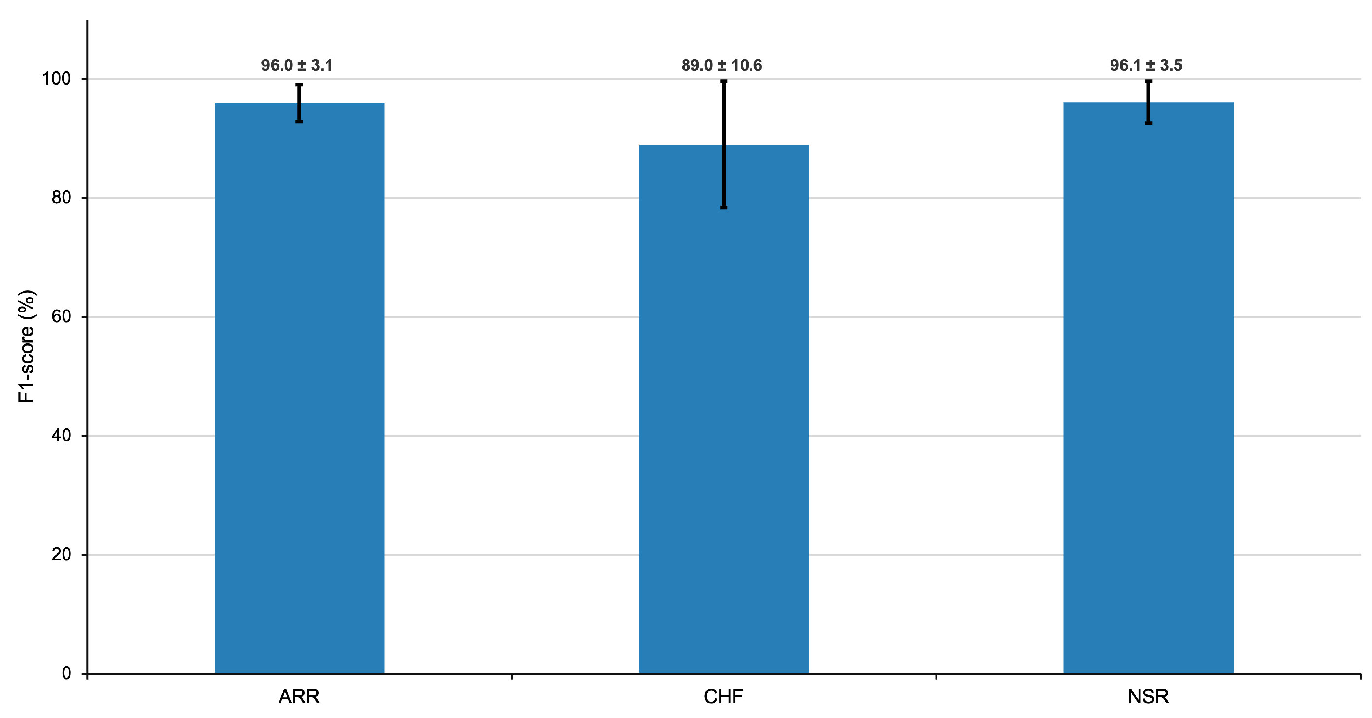
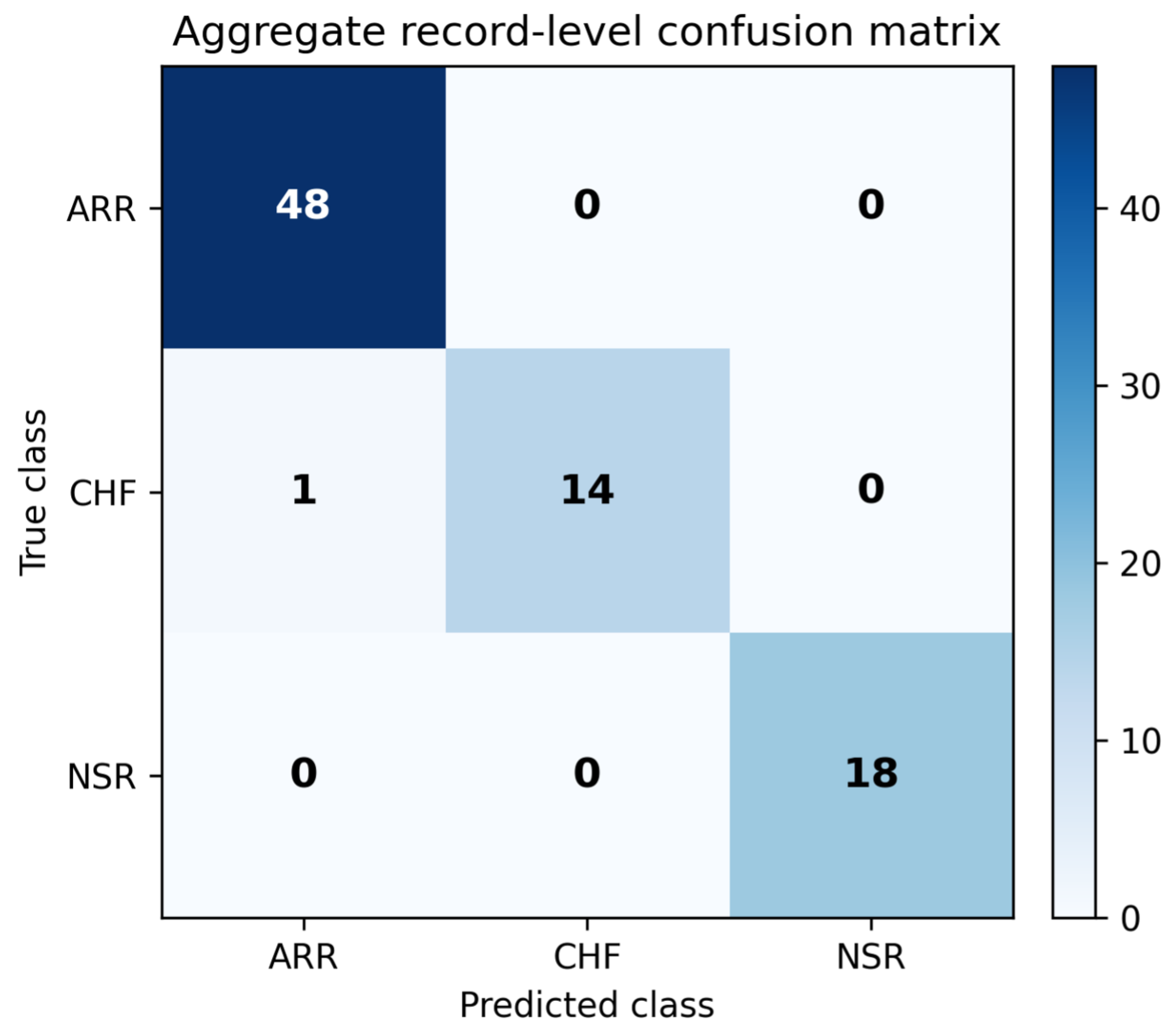
Quantitatively, the proposed method achieved 94.83% mean validation segment accuracy and 98.77% aggregate record-level accuracy across five record-level cross-validation folds. Compared with the stronger single-channel baseline, channel 2, early fusion improved aggregate record-level accuracy from 87.65% to 98.77%, an absolute improvement of 11.11 percentage points. Compared with channel 1, the improvement was 23.46 percentage points. This is stronger evidence than a comparison with the MathWorks reference workflow alone because all three models used the same data partitions, augmentation strategy and classifier configuration.

5.4. Limitations

The main limitation is the small number of independent records, especially CHF. Although segmenting produced thousands of images, the dataset contains only 81 reconstructed two-channel records and only 15 CHF records. This limits statistical certainty and makes class-wise estimates sensitive to individual records. Although the fusion model correctly classified 14 of the 15 CHF records, the Wilson confidence interval for CHF recall remained wide, so CHF-specific performance should be interpreted cautiously.

A further limitation is that the diagnostic labels are confounded with the PhysioNet source databases: ARR, CHF and NSR records originate from different databases. Although the proposed record-level splitting prevents segment-level leakage, it does not fully eliminate the possibility that the network learns source-specific acquisition or preprocessing characteristics rather than only clinical pathology. Future validation should use datasets in which multiple diagnostic classes are available within the same acquisition source, or clinically verified external datasets with consistent recording protocols.

Augmentation was intentionally conservative but still heuristic. The perturbation ranges were selected to represent small nuisance variation rather than diagnostic change: gain jitter represents amplitude calibration or electrode-contact variation; temporal shift represents segment-boundary uncertainty; mild time warping represents small rate or time-scale changes; baseline wander represents respiration, motion or electrode drift; and additive noise represents measurement contamination. The study did not include a full ablation of each augmentation component, nor did it assess calibration or uncertainty estimates. Finally, the study used GoogLeNet as a practical transfer-learning backbone. A purpose-built one-dimensional, two-dimensional or hybrid ECG model may outperform it, particularly for minority-class sensitivity.

5.5. Future Work

Future work should prioritise external validation on larger independent ECG datasets, with explicit patient-level separation wherever metadata permit it. Repeated cross-validation or nested cross-validation would provide more robust estimates if additional records become available. Model calibration, confidence intervals and decision-curve analysis would help determine whether the probability outputs are clinically meaningful rather than merely accurate.

Methodologically, several extensions are promising. Focal loss or class-balanced loss could be tested to improve CHF sensitivity without sacrificing precision. Cross-channel attention could be added to model relationships between the two scalogram panels explicitly. Explainability methods such as Grad-CAM could identify whether the network attends to plausible time–frequency regions associated with QRS morphology, rhythm variability or baseline behaviour. A verified clinical dataset containing true simultaneous multi-lead recordings should also be used to validate the early-fusion concept beyond the reconstructed ECGData derivative. Finally, the early-fusion concept could be evaluated in other modelling research such as Advanced Driver Assistance Systems (ADASs) and driver-state, where ECG, EDA and other biosignals may be combined for emotion and physiological-state inference.

5.6. Comparison with Selected Studies

Because the selected studies use different datasets, segmentation units and validation protocols, the comparison is methodological rather than a direct ranking of accuracy. The studies and their relevance to the present pipeline are summarised in

Table 10. Selected studies and methodological relevance to the present work. Direct numerical accuracy comparison is avoided because datasets, segmentation units and validation protocols differ.

Study	Representation/Model	Evaluation Emphasis	Relevance
Wang et al. (2021) [10]	CWT scalograms with CNN and RR features	Beat-level arrhythmia classification	Supports the value of wavelet time–frequency ECG images.
Toma and Choi (2022) [11]	Parallel recurrent and 2D-CNN branches using CWT scalograms	Imbalanced arrhythmia detection	Shows that combining temporal and scalogram information can improve imbalanced ECG classification.
MathWorks ECG workflow [12]	CWT RGB images with GoogLeNet/SqueezeNet transfer learning	ARR/CHF/NSR image classification	Closest practical starting point; present work adds source-file two-channel reconstruction, augmentation, single-channel ablation and record-level CV.
Yoon and Joo (2024) [8]	Generated 12-lead ECG from limited-lead input, ResNet classification	Multi-lead feasibility	Supports the claim that lead information can improve diagnostic classification.
Zhou and Fang (2025) [9]	Multi-scale hierarchical CNN with lead encoder attention	Multi-lead ECG classification	Highlights future direction beyond simple early image fusion.
Time-series deep learning and augmentation reviews [20,21,22]	General time-series classification and augmentation methods	Small-data deep learning and augmentation design	Supports the use of conservative signal-domain augmentation and careful validation in small time-series datasets.

.

6. Conclusions

This study proposed an early-fusion two-channel CWT-GoogLeNet pipeline for ECG classification and evaluated it using record-level cross-validation. Using the source-file row organisation to reconstruct the two separated ECG recordings, the method achieved 94.83% mean validation segment accuracy and 98.77% aggregate record-level accuracy for ARR, CHF and NSR classification. The same-split ablation showed that early fusion outperformed single-channel baselines under the same record-level folds, with aggregate record-level accuracy of 98.77% for early fusion compared with 75.31% for channel 1 and 87.65% for channel 2. These findings indicate that two-channel time–frequency fusion, conservative signal-domain augmentation, class-weighted learning and record-level evidence aggregation can improve the practical reliability of ECG classification on small biosignal datasets. However, the dataset remains small, the CHF class contains only 15 records, and diagnostic class is confounded with source database. External validation on larger clinically consistent multi-channel ECG datasets is therefore required before broader clinical deployment.