A Physics-Guided Graph Neural Network Framework for Predicting Organic Solar Cell Performance Parameters

Abstract

Organic solar cells (OSCs) have emerged as a competitive alternative to conventional silicon-based photovoltaics for their inexpensive production, versatility, and reduced energy consumption. However, it is still challenging to accurately assess their performance due to the complex interactions between molecular structure and device-level features. We provide a physics-constrained graph neural network (GNN) architecture for multi-output prediction of key OSC parameters, including power conversion efficiency (PCE), open-circuit voltage, short-circuit current density, and fill factor in this study. To ensure agreement between the anticipated PCE and its physically derived formulation, a physics-guided regularization term is added. Experimental results on a dataset of 5628 samples show that the neural-only GNN achieves strong predictive performance ($R^2=0.630$), outperforming the baseline model random forest ($R^2=0.537$). The proposed physics-constrained GNN maintains comparable accuracy ($R^2=0.626$) while significantly reducing physics violation (from 0.406 to 0.104). These results show that adding physics constraints makes predictions more consistent without lowering accuracy, making it a reliable way to predict OSC performance.

1. Introduction

1.1. Background and Motivation

Due to the negative environmental impacts of traditional fossil fuel-based energy sources, the usage of solar energy is growing quickly. Solar cells are an efficient and useful means of capturing solar energy, which is a consistent and abundant resource. The atmosphere receives 1367 W/m² of solar energy from the sun. Globally, about 1.81011 MW of solar energy is absorbed, which is enough to provide the world’s power needs [1,2]. Nevertheless, there are certain disadvantages to silicon-based photovoltaic cells, such as high energy production [3,4,5,6], a long energy payback time [7,8] and the bulky, heavy nature of silicon panels [9,10]. As a result, researchers and engineers are trying to create alternative photovoltaic technologies, like organic solar cells (OSCs), which can be made at low temperatures using solution-coating techniques. The manufacture of these emerging photovoltaic technologies is much less energy-intensive than that of traditional silicon photovoltaics, with an estimated energy consumption per watt of 0.26 kWh for silicon photovoltaics and only 0.02–0.07 kWh for OSCs [11,12]. Therefore, the photovoltaic industry’s carbon impact may be lessened by these alternative PV technologies [13]. Additionally, OSCs do not contain dangerous substances and may be made into flexible, lightweight panels that can be installed in locations where traditional silicon photovoltaics are unworkable [14,15,16,17,18]. Because of these characteristics, OSCs can be safely installed in modern cities with high electricity demand and limited rooftop space. As organic solar cells continue to advance, predicting their PCE is important for comparing them with inorganic cells and monitoring their development. Traditional prediction methods look at the electrical and structural features of the devices and simulate their current density–voltage (J-V) curves [19]. Simple equivalent circuit models help with comparisons, but they do not provide detailed information about the devices’ performance [20]. These traditional approaches are often slow and expensive because they need specific parameters for accurate results [21]. Analytical models and more complex simulations can explain charge transport better, but they are hard to use since it is difficult to get the required parameters [22]. To speed up the discovery of new, effective organic materials for photovoltaic technologies, efficient data-driven methods like machine learning are essential. Because OSC performance depends strongly on molecular structure and electronic interactions between donor and acceptor materials, machine learning models must capture both structural and physical information to generate reliable predictions.

1.2. Related Work

With the ability to predict device metrics such as PCE, energy levels, and other performance indicators based on experimental or chemical descriptors, machine learning has increasingly been used to accelerate the discovery of OSC materials [23,24]. As indicated by recent reviews, in an effort to reduce costs associated with experimental screening processes, OSC predictions have primarily utilized machine learning based on descriptors, for example, tree-based models or neural networks. However, these approaches mainly rely on manually designed numerical descriptors and often cannot fully capture the detailed molecular structure and interactions between donor and acceptor materials [25]. Given the fact that molecules can be naturally modeled using graph representations with atoms as nodes and chemical bonds as edges, GNNs provide a natural alternative for OSC prediction problems. An important part of this domain is provided by Gilmer et al.’s message-passing framework for graphs, which showed that graph-based learning can yield good results in molecular property predictions [22]. Thus, GNNs can be particularly effective for prediction in OSC systems, due to their ability to effectively leverage subtle differences between donor and acceptor molecules which can have substantial effect on device performance. Based on message-passing architecture, methods like Chemprop have shown very strong performance in molecular property prediction tasks, with numerous research works achieving highly accurate predictions (high $R^2$ scores) on benchmark datasets [26,27,28]. The drawback of purely data-driven models is that they may generate results that contradict physical phenomena. To improve prediction reliability, physics-guided learning incorporates known physical relationships into the model training process so that the predictions remain consistent with photovoltaic behavior. It was proposed by Raissi et al. in the form of physics-informed neural networks that incorporate known physical relationships in the optimization process, rather than relying solely on data [29]. Physics-informed approaches have recently attracted a lot of attention in photovoltaics, which is reflected in the emergence of physics-informed OSC performance prediction research [30]. Nevertheless, a major gap remains. OSC prediction research can be largely divided into two types, descriptor-based machine learning and physics-informed machine learning, with neither explicitly leveraging graph structure in the case of donor–acceptor pairs. At the same time, general molecular GNNs are trained exclusively to maximize accuracy, without any regard for physical properties [31]. To address this gap, this research introduces dual molecular graph representation and physics-consistency constraint for the simultaneous prediction of $V_{oc}$, $J_{sc}$, FF and PCE values.

Traditional ML models, especially random forest (RF), are extensively employed to forecast the behavior of OSCs because of their stability and ability to cope with nonlinearities. RF is an ensemble approach proposed by Leo Breiman that possesses good generalization ability and avoids overfitting in high dimensional feature spaces [32]. There are a number of examples where RF models successfully predict PCE in OPV systems based on the molecular descriptor representation and device-level parameters, yielding high prediction scores [33,34]. In a comparison study, RF-based models usually outperform linear regression and SVMs, especially when working with complex and non-uniform experimental data [35]. Moreover, RF methods were successfully used for donor–acceptor system identification in organic photovoltaics, suggesting the promise of RF-based approaches for predicting the behavior of high-performance materials [36]. An improvement of predictive performance can be achieved using DFT-derived features as an input [36]. However, RF methods are highly dependent on handcrafted features that fail to capture intrinsic structural information and thus underperform graph-based algorithms. Moreover, unlike GNNs, RF-based models do not take into account temporal properties of materials and thus are unable to capture the degradation of PCEs. We apply this model for comparing conventional baseline models with GNNs. Since other ML approaches are also feature-based methods exhibiting similar behavior when applied on a dataset with descriptors, other algorithms such as SVR and gradient boosting are not considered separately. Therefore, the aim of this work is to highlight the advantages of the proposed method in terms of incorporating molecular graph representation and physical constrains. Hence, the benefit of the proposed approach can be highlighted with just one reliable baseline method.

1.3. Research Gap and Objective

Despite recent improvements, there are still several problems with OSC performance prediction. Descriptor-based machine learning approaches, which mostly rely on manually generated features, sometimes overlook detailed molecular structural information. Although graph neural networks improve structural representation learning, most existing models optimize primarily for prediction accuracy without enforcing physical consistency across photovoltaic parameters. Forecasts may therefore be physically inconsistent even with high numerical precision.

Therefore, the objective of this work is to develop a physics-constrained graph neural network architecture that can simultaneously anticipate many OSC parameters while remaining consistent with known photovoltaic correlations.

1.4. Contribution

The main contribution of this paper is summarized as follows:

• We develop a physics-constrained GNN framework for multi-output prediction of OSC parameters, integrating molecular graph representations of D-A pairs with experimentally derived physical descriptors.
• We introduce a physics-guided regularization mechanism that enforces consistency between predicted PCE and its physically derived formulation based on $V_{oc}$, $J_{sc}$ and FF, improving the physical reliability of the model.
• We conduct a comparative evaluation against a random forest baseline and a neural-only GNN, demonstrating that the proposed approach achieves comparable predictive accuracy while significantly improving physical consistency.

2. Problem Formulation

This study formulates OSC performance prediction as a multi-output regression problem with a physics-consistency constraint. Each OSC sample consists of a donor–acceptor pair, physical descriptor features, and experimentally measured photovoltaic performance parameters.

2.1. Input Representation

Each OSC device is represented by a donor molecule D and an acceptor molecule A. The donor and acceptor are converted into molecular graphs as

$$G_D=(V_D,E_D),$$

(1)

$$G_A=(V_A,E_A),$$

(2)

where $G_D$ and $G_A$ denote the donor and acceptor molecular graphs, respectively. $V_D$ and $V_A$ represent the atom/node sets, while $E_D$ and $E_A$ represent the chemical bond/edge sets.

In addition to graph-based molecular representations, each sample includes a physical descriptor vector:

$${\mathbf{f}}_{phys}=[E_{\mathrm{HOMO}}^D,E_{\mathrm{LUMO}}^D,E_{\mathrm{HOMO}}^A,E_{\mathrm{LUMO}}^A,E_g^D,E_g^A,\Delta E_{\mathrm{HOMO}},\Delta E_{\mathrm{LUMO}}],$$

(3)

where $E_{\mathrm{HOMO}}^D$ and $E_{\mathrm{LUMO}}^D$ are the HOMO and LUMO energy levels of the donor, $E_{\mathrm{HOMO}}^A$ and $E_{\mathrm{LUMO}}^A$ are the HOMO and LUMO energy levels of the acceptor, $E_g^D$ and $E_g^A$ are the donor and acceptor bandgaps, and $\Delta E_{\mathrm{HOMO}}$ and $\Delta E_{\mathrm{LUMO}}$ denote the corresponding donor–acceptor energy offsets [37,38].

Thus, the complete input for the i-th OSC sample is defined as

$$X_i=\left(G_D^{\left(i\right)},G_A^{\left(i\right)},{\mathbf{f}}_{phys}^{\left(i\right)}\right).$$

(4)

2.2. Output Targets

The target vector contains four experimentally measured OSC performance parameters:

$$Y_i=\left[V_{oc}^{\left(i\right)},J_{sc}^{\left(i\right)},F{F}^{\left(i\right)},PC{E}^{\left(i\right)}\right],$$

(5)

where $V_{oc}$ is the open-circuit voltage, $J_{sc}$ is the short-circuit current density, $FF$ is the fill factor, and $PCE$ is the power conversion efficiency.

The prediction function is defined as

$${\widehat{Y}}_i=f_{\theta }\left(X_i\right)=\left[{\widehat{V}}_{oc}^{\left(i\right)},{\widehat{J}}_{sc}^{\left(i\right)},{\widehat{FF}}^{\left(i\right)},{\widehat{PCE}}^{\left(i\right)}\right],$$

(6)

where $f_{\theta }(·)$ denotes the proposed learning model parameterized by $\theta$, and the hat symbol represents predicted values.

2.3. Physics-Consistency Constraint

The power conversion efficiency of a solar cell is physically related to $V_{oc}$, $J_{sc}$, and $FF$ as

$$PCE={\displaystyle \frac{V_{oc}·J_{sc}·FF}{P_{in}}},$$

(7)

where $P_{in}$ is the incident optical input power density under standard illumination conditions. In the dataset used in this study, PCE is reported in percentage form, and $P_{in}$ is treated as a constant normalization factor.

Accordingly, the physically reconstructed PCE [39] from model predictions is defined as

$${\widehat{PCE}}_{phys}^{\left(i\right)}={\displaystyle \frac{{\widehat{V}}_{oc}^{\left(i\right)}·{\widehat{J}}_{sc}^{\left(i\right)}·{\widehat{FF}}^{\left(i\right)}}{P_{in}}}.$$

(8)

This formulation allows the model to compare the directly predicted ${\widehat{PCE}}^{\left(i\right)}$ with the physically reconstructed ${\widehat{PCE}}_{phys}^{\left(i\right)}$.

2.4. Learning Objective

The total training objective combines a supervised prediction loss and a physics-consistency loss:

$${\mathcal{L}}_{total}={\mathcal{L}}_{task}+\lambda {\mathcal{L}}_{physics},$$

(9)

where $\lambda$ is a non-negative weighting coefficient that controls the influence of the physics-consistency term.

The supervised task loss is defined as

$${\mathcal{L}}_{task}={\displaystyle \frac{1}{N}}{\displaystyle \sum _{i=1}^N}\mathrm{Huber}\left(Y_i,{\widehat{Y}}_i\right),$$

(10)

where N is the number of training samples and $\mathrm{Huber}(·)$ denotes the Huber regression loss.

The physics-consistency loss is defined as

$${\mathcal{L}}_{physics}={\displaystyle \frac{1}{N}}{\displaystyle \sum _{i=1}^N}\mathrm{Huber}\left({\widehat{PCE}}^{\left(i\right)},{\widehat{PCE}}_{phys}^{\left(i\right)}\right).$$

(11)

This loss penalizes disagreement between the directly predicted PCE and the PCE reconstructed from the predicted photovoltaic parameters.

2.5. Optimization Problem

Given a dataset [40]

$$\mathcal{D}={\left\{\left(X_i,Y_i\right)\right\}}_{i=1}^N,$$

(12)

the objective is to learn optimal model parameters ${\theta }^{*}$ by solving

$${\theta }^{*}=\arg \underset{\theta }{\min }{\displaystyle \frac{1}{N}}{\displaystyle \sum _{i=1}^N}\left[{\mathcal{L}}_{task}^{\left(i\right)}+\lambda {\mathcal{L}}_{physics}^{\left(i\right)}\right].$$

(13)

This formulation enables the model to learn accurate multi-output predictions while encouraging consistency with the photovoltaic efficiency relationship.

3. Proposed Method

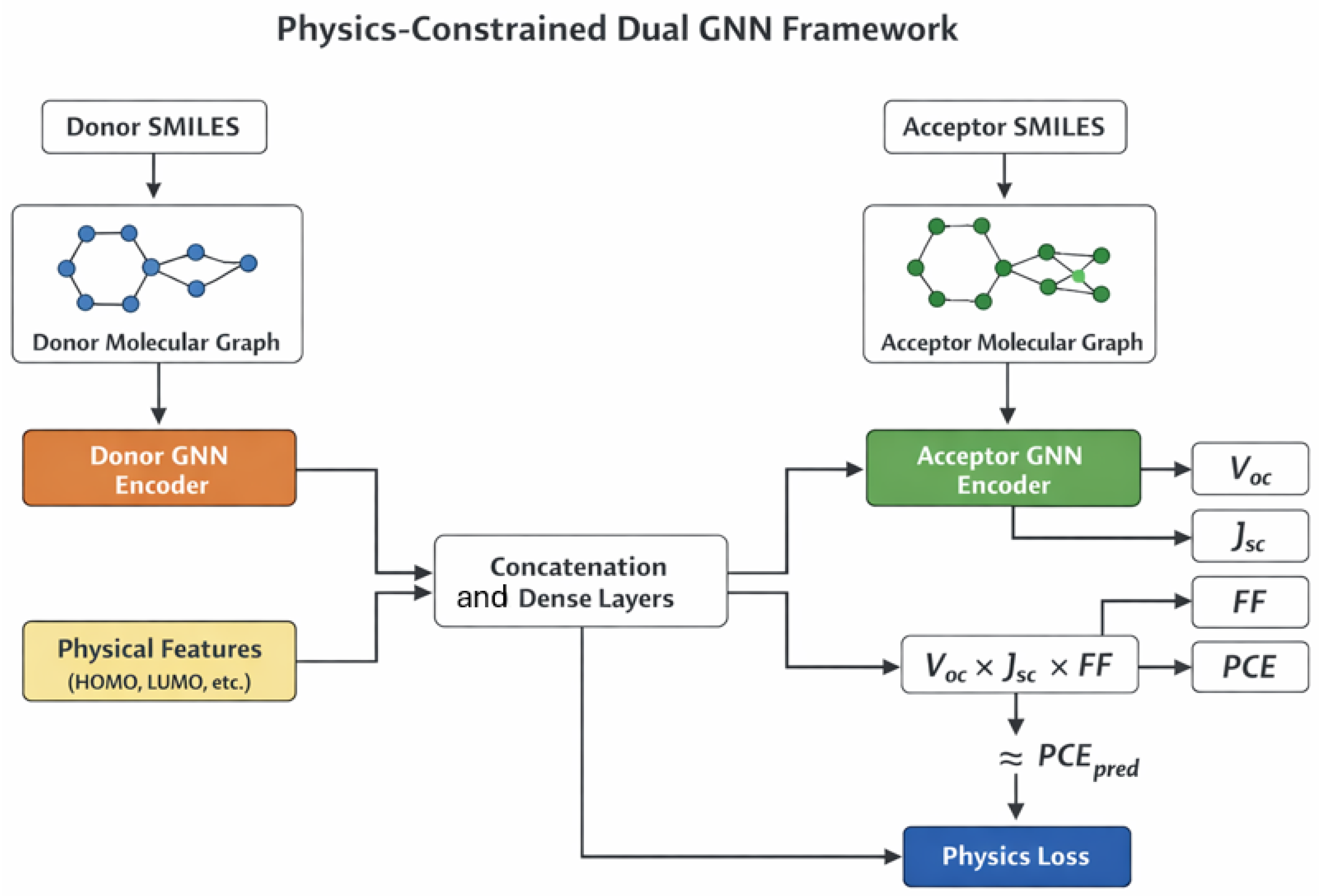
The suggested framework’s fundamental architecture is depicted in Figure 1. The model is built to enforce consistency across predicted photovoltaic parameters while simultaneously learning from physical and molecular structural descriptors.

3.1. Feature Encoding

Each sample is represented by a vector of physical characteristics and two molecular graphs that correspond to the donor and acceptor. The model is able to capture complementary information because structural and physical inputs are separated: physical descriptors offer global electronic features, while graph representations reflect local atomic interactions and bonding structure. In OSC systems, where device performance is dependent on both molecular structure and energy-level alignment between donor and acceptor materials, this hybrid representation is especially crucial. The model can learn more comprehensive and insightful feature representations by integrating these inputs.

3.2. Dual-Graph Encoding and Fusion

Two parallel GNN encoders extract features independently from the donor graph and the acceptor graph. This architecture allows the model to create separate representations of each component because it takes into account their unique roles in the material. Following the collection of information about the neighbors through message passing, each encoder conducts a pooling step to generate a vector representation. Then, the vector representations are merged with the modified physical characteristics. This merging process is crucial to the model’s capacity to capture the complex dependencies in OSC behavior.

3.3. Multiple Target Prediction

The target variables will be predicted at the same time when training the multi-output model. Compared to using separate prediction models, the joint learning method boosts the model’s ability to generalize. This is because it lets the model leverage the relationships between the photovoltaic features. Another advantage of the joint learning framework is that it highlights task similarities, which helps reduce redundancy.

3.4. Physics-Guided Regularization

The proposed framework incorporates a physics-guided regularization mechanism based on the photovoltaic efficiency relationship defined in Equation (7). Instead of treating $V_{oc}$, $J_{sc}$, $FF$, and $PCE$ as completely independent prediction targets, the model enforces consistency between the directly predicted PCE and the physically reconstructed PCE obtained from the predicted photovoltaic parameters.

Using the predicted values ${\widehat{V}}_{oc}$, ${\widehat{J}}_{sc}$, and $\widehat{FF}$, the model computes a reconstructed efficiency value ${\widehat{PCE}}_{phys}$ according to Equation (8). During training, the disagreement between the directly predicted $\widehat{PCE}$ and the reconstructed ${\widehat{PCE}}_{phys}$ is minimized through the physics-consistency loss defined in Equation (11).

This approach adds a physically meaningful consistency constraint to the learning objective, in contrast to solely data-driven optimization. As a result, the model is encouraged to produce predictions that are both consistent with the underlying photovoltaic relationship among the projected parameters and minimize regression error. The framework maintains flexibility while enhancing physical reliability and prediction stability because the physics element functions as a soft regularization constraint rather than a hard restriction.

3.5. Optimization Strategy

Gradient-based optimization with a composite loss function that includes physics regularization and prediction error is used to train the model. A weighting parameter allows for a balance between predictive accuracy and physical consistency. Mini-batch optimization updates model parameters during training, and validation performance is monitored to prevent overfitting. This training method maintains generalization capacity while ensuring steady convergence.

3.6. Algorithm Design

The primary computational flow of the suggested architecture is highlighted in Algorithm 1. The physical descriptor branch introduces electronic information that might not be directly recovered from topology alone, while the donor and acceptor graphs are encoded independently to maintain their unique structural responsibilities. These diverse representations can interact prior to prediction because of the fusion layer. The physics-guided optimization step is where a neural-only GNN differs most. The technique uses the projected $V_{oc}$, $J_{sc}$, and $FF$ to regularize PCE rather than considering it as a completely independent goal. This reduce physically implausible outputs and improves the learning process’s consistency with OSC device behavior.

Algorithm 1: Training and Inference of the Physics-Constrained Dual GNN

4. Experimental Setup

In this section, we have discussed the dataset, data preprocessing, model configuration, training details, and evaluation metrics.

4.1. Dataset Description

The OSC dataset contains 5628 donor-acceptor pairs, along with experimentally measured photovoltaic performance parameters and physically meaningful electronic descriptors [41]. Each sample consists of molecular graph representations derived from SMILES strings and structured numerical descriptors related to molecular energy levels and photovoltaic behavior.

Table 1. Description of the primary attributes used in the OSC dataset.

Attribute	Description	Type
SMILES	Molecular representation of donor/acceptor molecules	String
$E_{\mathrm{HOMO}}$	Highest occupied molecular orbital energy level	Continuous
$E_{\mathrm{LUMO}}$	Lowest unoccupied molecular orbital energy level	Continuous
$E_g$	Molecular bandgap energy	Continuous
$\Delta E_{\mathrm{HOMO}}$	HOMO energy offset between donor and acceptor	Continuous
$\Delta E_{\mathrm{LUMO}}$	LUMO energy offset between donor and acceptor	Continuous
$V_{oc}$	Open-circuit voltage	Continuous
$J_{sc}$	Short-circuit current density	Continuous
$FF$	Fill factor	Continuous
$PCE$	Power conversion efficiency	Continuous

summarizes the primary attributes used in this study, including their physical meaning and structural characteristics. The dataset includes both graph-based molecular representations and continuous numerical descriptors, enabling the model to jointly learn structural and electronic information.

To better understand the dataset distribution and variability, statistical properties of the target photovoltaic parameters are summarized in

Table 2. Statistical summary of the target photovoltaic parameters.

Parameter	Mean	Std	Min	Max
$V_{oc}$	0.813	0.137	0.020	1.320
$J_{sc}$	10.607	5.928	0.020	29.830
$FF$	0.539	0.124	0.100	0.797
$PCE$	5.149	3.798	0.001	18.570

. The dataset spans a broad range of OSC performance values, allowing the proposed framework to generalize across diverse donor–acceptor systems.

The statistical summary indicates substantial variability across the photovoltaic parameters, demonstrating the diversity of the OSC systems included in the dataset. Such variability is important for evaluating the generalization capability of machine learning models across different donor–acceptor combinations.

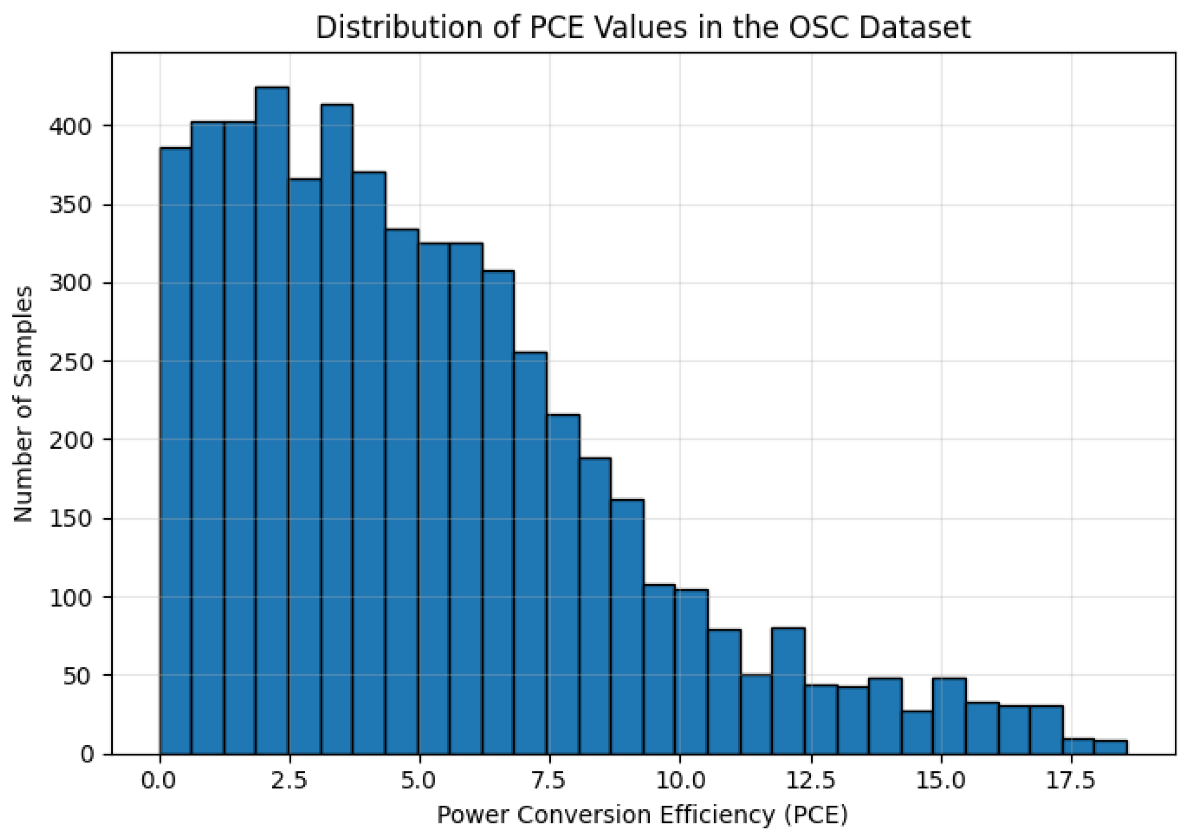
The PCE distribution shown in Figure 2 demonstrates that the dataset covers both low-efficiency and high-efficiency OSC systems. The distribution is moderately right-skewed, with a larger concentration of samples in the low-to-medium PCE range and fewer high-efficiency samples. Such variability is beneficial for evaluating the generalization capability of machine learning models across diverse OSC device configurations.

4.2. Data Preprocessing

Simplified molecular input line entry system (SMILES) strings represent the donor and acceptor molecules. These strings are transformed into graph structures, with atoms as nodes and chemical bonds as edges [42]. To encode atomic level attributes, we extracted node features. We also used structured physical descriptors as numerical features alongside graph inputs. Standard scaling normalizes all continuous features to ensure steady training and improved convergence. To maintain data quality, we removed samples with missing or incorrect entries.

4.3. Data Splitting

A random split was used to separate the dataset into training, validation, and test sets. In particular, 80% of the data was used for training, 10% for validation, and 10% for testing [43]. The test set was set aside for the final performance assessment, and the validation set was used for model selection and hyperparameter tuning.

4.4. Model Configuration

The proposed model consists of two parallel GNN encoders, one for the donor graph and one for the acceptor graph. Each encoder contains two graph convolutional layers followed by ReLU activation and global mean pooling to obtain fixed-length molecular embeddings. The donor and acceptor embeddings are concatenated with the multi-layer perception (MLP)-transformed physical descriptor vector [44,45,46]. The fused representation is then passed through fully connected layers to predict $V_{oc}$, $J_{sc}$, FF, and PCE simultaneously.

4.5. Training Parameters and Details

The proposed physics-constrained GNN was implemented using PyTorch v2.10.0+cu128 and PyTorch Geometric v2.7.0. The dataset was divided into training, validation, and testing. All continuous features were normalized prior to training. The graph neural network encoder employed two graph convolution layers followed by global mean pooling and fully connected regression layers for multi-output prediction. The hidden feature dimension was set to 128, and ReLU activation functions were used throughout the network. The model was optimized using the Adam optimizer with a learning rate of 0.001 and a batch size of 32. Training was performed for 100 epochs. For the physics-constrained GNN, the physics-consistency weighting coefficient $\lambda$ was experimentally selected as 0.05 based on the trade-off between predictive accuracy and physics violation reduction. The Huber loss function was used for both the supervised regression loss and the physics-consistency regularization term. The model configuration and training parameters are summarized in

Table 3. Model configuration and training parameters.

Parameter	Value
Hidden dimension	128
Number of GNN layers	2
Activation function	ReLU
Optimizer	Adam
Learning rate	0.001
Batch size	32
Epochs	100
Loss function	Huber Loss
Physics coefficient ($\lambda$)	0.05
Train/Validation/Test split	80/10/10

.

4.6. Evaluation Metrics

Model performance was evaluated using root mean square (RMSE), mean absolute error (MAE), and coefficient of determination ($R^2$) [47]. In addition to standard regression metrics, a physics consistency metric is used to quantify the deviation from the physical relationship among predicted parameters, which is

$$\widehat{PCE}=({\widehat{J}}_{sc}·{\widehat{V}}_{oc}·\widehat{FF})$$

this metric provides the model’s adherence measurement to the underlying physical constraints.

5. Results and Discussion

Table 4. Performance comparison of different models for PCE prediction.

Model	Physics Violation	MAE	RMSE	${\mathit{R}}^2$
Random Forest	0.307	1.913	2.596	0.537
Neural GNN	0.406	1.745	2.321	0.630
Physics GNN ($\lambda =0.05$)	0.104	1.805	2.334	0.626

summarizes the examined models’ prediction performance. The RF model’s descriptor-based formulation restricts its capacity to capture intricate structural interactions between donor–acceptor molecular systems, despite the model’s respectable prediction performance. RF is unable to immediately learn the molecular connection patterns and local atomic interactions that significantly affect photovoltaic activity in organic solar cells because it is only dependent on manually created numerical descriptions. As a result, its overall predictive performance is still inferior than graph-based methods.

According to Table 4, the RF model has the greatest RMSE value and an $R^2$ score of 0.537 out of all the models that were examined. This suggests that the model’s ability to generalize complex OSC structure–property connections is restricted. On the other hand, by directly learning chemical representations from donor and acceptor graph topologies, both GNN-based models show enhanced predictive capability. The neural GNN outperforms the other models in terms of prediction, with an $R^2$ score of 0.630 and lower RMSE values when compared to the RF baseline. These findings suggest that the nonlinear structural and electrical linkages controlling OSC performance are better captured by graph-based learning. The enhancement further implies that compared to traditional descriptor-based methods, molecular graph representations offer richer and more informative characteristics. An ablation analysis of the suggested physics-guided regularization technique is also provided by contrasting the neural GNN with the physics-constrained GNN. The neural GNN merely maximizes the regression objective and attains marginally improved prediction accuracy when the physics-consistency factor is absent. However, this solely data-driven optimization leads to a higher level of physics violation. The suggested framework considerably lowers the physics inconsistency while retaining similar predictive performance after adding the physics-guided regularization term. This behavior shows that the incorporation of the PV consistency constraint into the learning objective is responsible for the improvement rather than architectural complexity alone. The suggested physics-constrained GNN offers noticeably better physical reliability, despite the neural GNN’s somewhat higher predictive accuracy. In particular, the physics violation measure significantly drops from 0.406 in the neural GNN to 0.104 in the suggested framework. This decrease suggests that there is more agreement between the anticipated values and the underlying photovoltaic efficiency relationship. Thus, instead of optimizing only for numerical regression accuracy, the suggested physics-guided regularization effectively limits the learning process toward physically valid predictions.

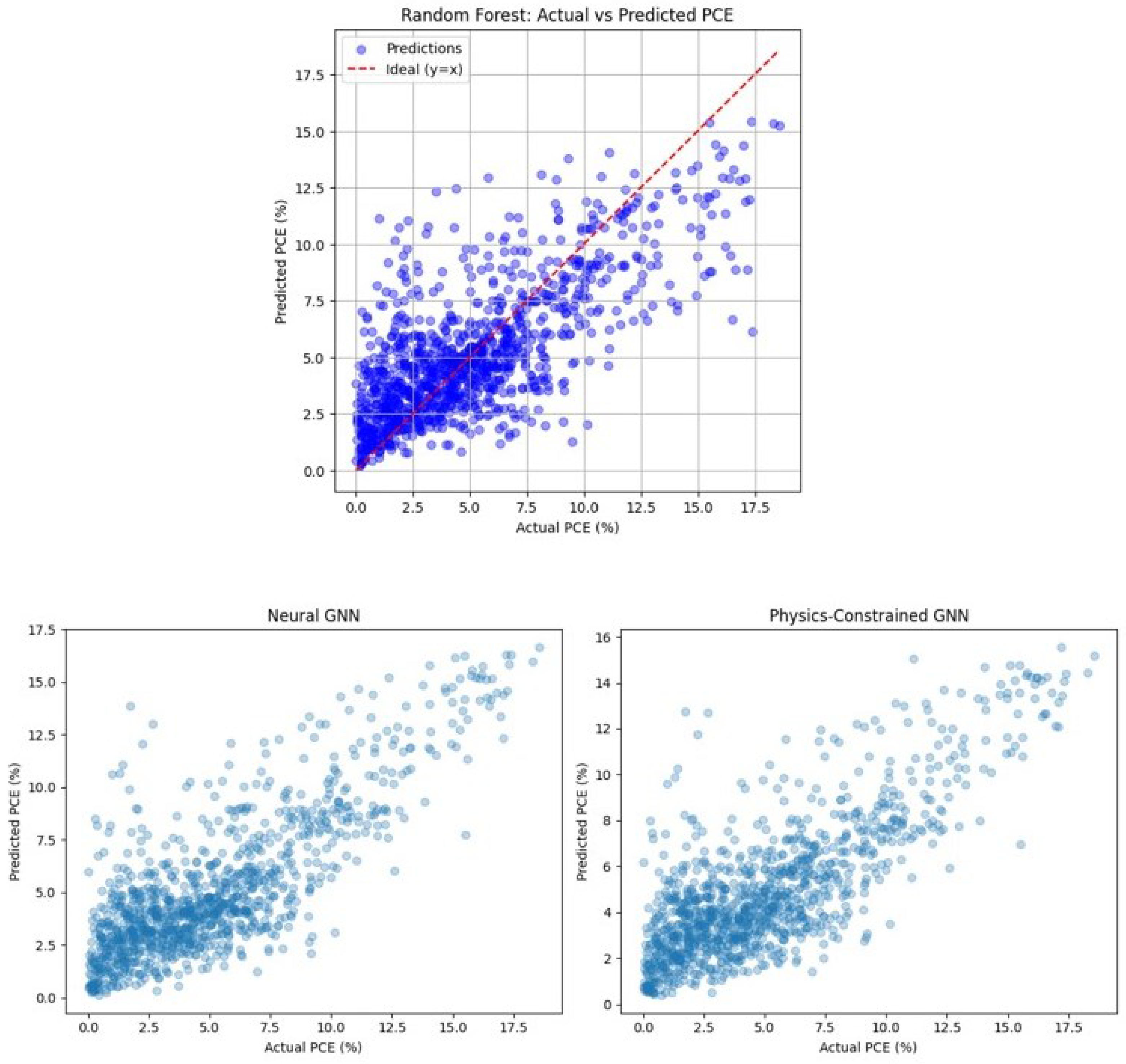
Figure 3 illustrates the relationship between actual and predicted PCE values. The neural-only and physics-constrained GNN models show strong agreement with the ground truth, while the random forest model exhibits larger deviations. The adherence to the underlying physical relationship among projected parameters is a crucial distinction between the physics-constrained and neural-only models. Physically contradictory predictions may arise from the neural-only GNN’s autonomous treatment of each target. The suggested model, on the other hand, incorporates a physics-guided regularization term that guarantees consistency between the anticipated PCE and its constituent variables. Consequently, the physics constrained GNN dramatically lowers the departure from the anticipated physical relationship, indicating increased prediction dependability.

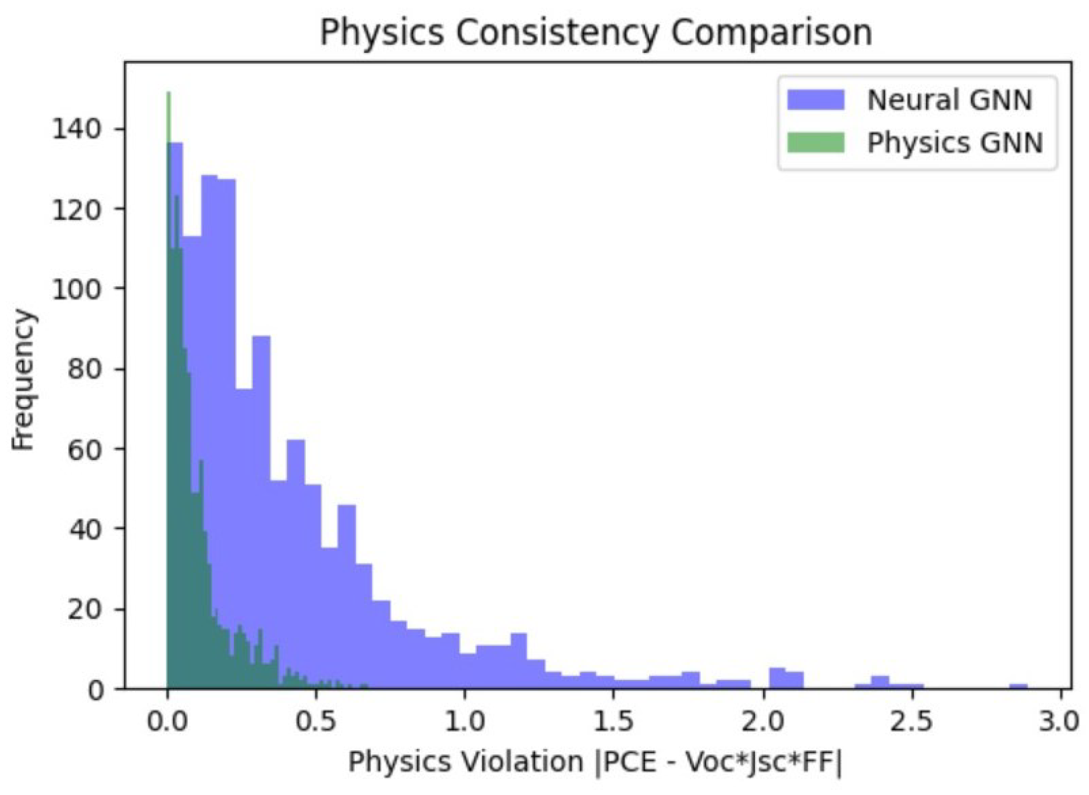
The distribution of physics violations for the neural-only and physics-constrained models is compared in Figure 4. Large discrepancies are evident in the neural-only GNN’s wide distribution and lengthy tail. The physics constrained model, on the other hand, yields a densely concentrated distribution close to zero, indicating that the majority of predictions meet the physical relationship. This outcome demonstrates that the suggested approach enhances both overall prediction stability and average consistency. The results of the experiment show a trade-off between physical uniformity and prediction accuracy. The neural-only GNN does not impose any physical relationship among the predicted parameters, despite achieving the best accuracy. The suggested model greatly improves physical consistency while maintaining almost the same predictive performance by adding a physics constraint. This balance is controlled by the weighting parameter $\lambda$, and a suitable value allows the model to produce predictions that are both highly accurate and physically meaningful. In practical applications, where physically inconsistent predictions might result in untrustworthy conclusions despite high numerical accuracy, this trade-off is crucial.

The investigation of the physics-consistency weighting coefficient $\lambda$ provides more insight into the trade-off between physical consistency and prediction accuracy. The model gets the maximum predicted accuracy and operates as a totally data-driven neural GNN when $\lambda =0$, but it also shows the most physical discrepancy. The physics-guided regularization strengthens with increasing $\lambda$, resulting in a significant decrease in the physics violation metric. According to experimental findings, $\lambda =0.05$ offers the optimum compromise between physical consistency and predictive performance, preserving competitive regression accuracy while greatly enhancing agreement with the photovoltaic connection. The suggested framework shows enhanced capacity for learning molecular structure–property relationships while concurrently preserving physical consistency among predicted photovoltaic parameters when compared to traditional descriptor-based machine learning techniques frequently employed in OSC prediction studies. The suggested graph-based system uses graph message propagation to directly capture molecular topology and local atomic interactions, in contrast to conventional regression models that solely rely on manually created descriptors. Additionally, by enhancing agreement with established photovoltaic connections, the incorporation of physics-guided regularization sets the suggested method apart from solely data-driven GNN models.

Overall, the findings show that combining physics-guided regularization with graph-based molecular representation learning enhances the physical consistency and predictive reliability of OSC performance prediction. The suggested framework offers a more balanced and physically understandable learning technique for solar materials modeling, even though purely data-driven models might achieve slightly higher numerical accuracy.

6. Conclusions

This work introduces a physics-informed graph neural network framework designed to predict multiple performance characteristics of OSCs. The model brings together molecular graph representations of donor–acceptor pairs with physically meaningful descriptors, allowing it to capture both structural and electrical properties effectively. To maintain consistency across predicted outputs—and to respect the inherent physical relationships among $V_{oc}$, $J_{sc}$, FF, and PCE-a physics-based regularization term is incorporated. Experimental results show that graph-based approaches outperform traditional machine learning methods, highlighting the value of learning from molecular structure. While a purely neural GNN achieves the highest predictive accuracy, it often produces results that violate known physical relationships. In contrast, the proposed physics-constrained model strikes a better balance, reducing such inconsistencies while maintaining strong predictive performance. The suggested framework performs well; however, there are still a number of drawbacks. First, the physics-guided regularization is predicated on continuous incoming illumination circumstances and an approximate photovoltaic consistency relationship. Second, the suggested model relies on the availability of both empirically derived physical descriptors and molecular graph representations, which may not always be available for recently synthesized materials. Furthermore, the methodology has only been tested on one OSC dataset; more research is needed to determine whether it can be used to larger and more varied solar datasets. Future research will concentrate on expanding the framework to include more extensive photovoltaic material systems, enhancing descriptor independence, and adding more thorough physical formulations.

Overall, the study demonstrates that integrating domain knowledge into deep learning models leads to more reliable and interpretable predictions. This approach offers a promising direction for physically consistent machine learning in materials science and could be extended to other applications where relationships between target variables are well understood.

References

1. Oni, A.M.; Mohsin, A.S.; Rahman, M.M.; Bhuian, M.B.H. A comprehensive evaluation of solar cell technologies, associated loss mechanisms, and efficiency enhancement strategies for photovoltaic cells. Energy Rep. 2024, 11, 3345–3366. [Google Scholar] [CrossRef]
2. Biswas, S.K.; Mim, M.K.; Ahmed, M. Design and Simulation of an Environment-Friendly ZrS2/CuInS2 Thin Film Solar Cell Using SCAPS 1D Software. Adv. Mater. Sci. Eng. 2023, 2023, 8845555. [Google Scholar] [CrossRef]
3. Anctil, A.; Babbitt, C.W.; Raffaelle, R.P.; Landi, B.J. Cumulative energy demand for small molecule and polymer photovoltaics. Prog. Photovolt. Res. Appl. 2013, 21, 1541–1554. [Google Scholar] [CrossRef]
4. Anctil, A.; Lee, E.; Lunt, R.R. Net energy and cost benefit of transparent organic solar cells in building-integrated applications. Appl. Energy 2020, 261, 114429. [Google Scholar] [CrossRef]
5. Zhou, Z.; Carbajales-Dale, M. Assessing the photovoltaic technology landscape: Efficiency and energy return on investment (EROI). Energy Environ. Sci. 2018, 11, 603–608. [Google Scholar] [CrossRef]
6. García-Valverde, R.; Cherni, J.A.; Urbina, A. Life cycle analysis of organic photovoltaic technologies. Prog. Photovolt. Res. Appl. 2010, 18, 535–558. [Google Scholar] [CrossRef]
7. Roes, A.L.; Alsema, E.A.; Blok, K.; Patel, M.K. Ex-ante environmental and economic evaluation of polymer photovoltaics. Prog. Photovolt. Res. Appl. 2009, 17, 372–393. [Google Scholar] [CrossRef]
8. Heeger, A.J. 25th anniversary article: Bulk heterojunction solar cells: Understanding the mechanism of operation. Adv. Mater. 2014, 26, 10–28. [Google Scholar] [CrossRef]
9. Lewis, N.S. Toward cost-effective solar energy use. Science 2007, 315, 798–801. [Google Scholar] [CrossRef]
10. Jean, J.; Brown, P.R.; Jaffe, R.L.; Buonassisi, T.; Bulović, V. Pathways for solar photovoltaics. Energy Environ. Sci. 2015, 8, 1200–1219. [Google Scholar] [CrossRef]
11. Martin, B.; Amos, D.; Brehob, E.; van Hest, M.F.; Druffel, T. Techno-economic analysis of roll-to-roll production of perovskite modules using radiation thermal processes. Appl. Energy 2022, 307, 118200. [Google Scholar] [CrossRef]
12. Osedach, T.P.; Andrew, T.L.; Bulović, V. Effect of synthetic accessibility on the commercial viability of organic photovoltaics. Energy Environ. Sci. 2013, 6, 711–718. [Google Scholar] [CrossRef]
13. Mim, M.K.; Biswas, S.K. Performance Analysis of Sr3SbI3-Based Perovskite Solar Cell Using SCAPS-1D Software. Adv. Mater. Sci. Eng. 2025, 2025, 7134012. [Google Scholar] [CrossRef]
14. Carlson, D.E.; Wronski, C.R. Amorphous silicon solar cells. In Practical Handbook of Photovoltaics; Elsevier Science: Amsterdam, The Netherlands, 2003; pp. 281–315. [Google Scholar] [CrossRef]
15. Lungenschmied, C.; Dennler, G.; Neugebauer, H.; Sariciftci, S.N.; Glatthaar, M.; Meyer, T.; Meyer, A. Flexible, long-lived, large-area, organic solar cells. Sol. Energy Mater. Sol. Cells 2007, 91, 379–384. [Google Scholar] [CrossRef]
16. Brus, V.V.; Lee, J.; Luginbuhl, B.R.; Ko, S.J.; Bazan, G.C.; Nguyen, T.Q. Solution-processed semitransparent organic photovoltaics: From molecular design to device performance. Adv. Mater. 2019, 31, 1900904. [Google Scholar] [CrossRef]
17. Forberich, K.; Guo, F.; Bronnbauer, C.; Brabec, C.J. Efficiency limits and color of semitransparent organic solar cells for application in building-integrated photovoltaics. Energy Technol. 2015, 3, 1051–1058. [Google Scholar] [CrossRef]
18. Park, S.; Heo, S.W.; Lee, W.; Inoue, D.; Jiang, Z.; Yu, K.; Jinno, H.; Hashizume, D.; Sekino, M.; Yokota, T.; et al. Self-powered ultra-flexible electronics via nano-grating-patterned organic photovoltaics. Nature 2018, 561, 516–521. [Google Scholar] [CrossRef]
19. Koster, L.J.A.; Mihailetchi, V.D.; Ramaker, R.; Blom, P.W.M. Light intensity dependence of open-circuit voltage of polymer:fullerene solar cells. Appl. Phys. Lett. 2005, 86, 123509. [Google Scholar] [CrossRef]
20. Hossain, N.; Das, S.; Alford, T.L. Equivalent circuit modification for organic solar cells. Circuits Syst. 2015, 6, 153–160. [Google Scholar] [CrossRef]
21. Li, Y.; Huang, W.; Zhao, D.; Wang, L.; Jiao, Z.; Huang, Q.; Wang, P.; Sun, M.; Yuan, G. Recent progress in organic solar cells: A review on materials from acceptor to donor. Molecules 2022, 27, 1800. [Google Scholar] [CrossRef] [PubMed]
22. Guermoui, M.; Rabehi, A. Soft computing for solar radiation potential assessment in Algeria. Int. J. Ambient Energy 2020, 41, 1524–1533. [Google Scholar] [CrossRef]
23. Seifrid, M.; Lo, S.; Choi, D.G.; Tom, G.; Le, M.L.; Li, K.; Sankar, R.; Vuong, H.T.; Wakidi, H.; Yi, A.; et al. Beyond molecular structure: Critically assessing machine learning for designing organic photovoltaic materials and devices. J. Mater. Chem. A 2024, 12, 14540–14558. [Google Scholar] [CrossRef]
24. Lee, J.; Ban, H.; Seo, H.; Lee, H.; Arshad, F.; Kim, D. Structure-guided machine learning for efficiency prediction of organic photovoltaics using experimentally informed molecular descriptors. Digit. Discov. 2026, 5, 1510–1521. [Google Scholar] [CrossRef]
25. Ahmed, D.R.; Muhammadsharif, F.F. A Review of Machine Learning in Organic Solar Cells. Processes 2025, 13, 393. [Google Scholar] [CrossRef]
26. Gilmer, J.; Schoenholz, S.S.; Riley, P.F.; Vinyals, O.; Dahl, G.E. Neural Message Passing for Quantum Chemistry. In Proceedings of the 34th International Conference on Machine Learning; Proceedings of Machine Learning Research: Cambridge, MA, USA, 2017; Volume 70, pp. 1263–1272. [Google Scholar]
27. Yang, K.; Swanson, K.; Jin, W.; Coley, C.W.; Eiden, P.; Gao, H.; Guzman-Perez, A.; Hopper, T.; Kelley, B.; Mathea, M.; et al. Analyzing Learned Molecular Representations for Property Prediction. J. Chem. Inf. Model. 2019, 59, 3370–3388. [Google Scholar] [CrossRef]
28. Wu, Z.; Ramsundar, B.; Feinberg, E.N.; Gomes, J.; Geniesse, C.; Pappu, A.S.; Leswing, K.; Pande, V. MoleculeNet: A Benchmark for Molecular Machine Learning. Chem. Sci. 2018, 9, 513–530. [Google Scholar] [CrossRef]
29. Reiser, P.; Neubert, M.; Eberhard, A.; Torresi, L.; Zhou, C.; Shao, C.; Metni, H.; van Hoesel, C.; Schopmans, H.; Sommer, T.; et al. Graph neural networks for materials science and chemistry. Commun. Mater. 2022, 3, 93. [Google Scholar] [CrossRef]
30. Raissi, M.; Perdikaris, P.; Karniadakis, G.E. Physics-informed neural networks: A deep learning framework for solving forward and inverse problems involving nonlinear partial differential equations. J. Comput. Phys. 2019, 378, 686–707. [Google Scholar] [CrossRef]
31. Khatua, R.; Das, B.; Mondal, A. Physics-Informed Machine Learning with Data-Driven Equations for Predicting Organic Solar Cell Performance. ACS Appl. Mater. Interfaces 2024, 16, 57467–57480. [Google Scholar] [CrossRef] [PubMed]
32. Breiman, L. Random Forests. Mach. Learn. 2001, 45, 5–32. [Google Scholar] [CrossRef]
33. Eibeck, A.; Nurkowski, D.; Menon, A.; Bai, J.; Wu, J.; Zhou, L.; Mosbach, S.; Akroyd, J.; Kraft, M. Predicting Power Conversion Efficiency of Organic Photovoltaics: Models and Data Analysis. ACS Omega 2021, 6, 23764–23775. [Google Scholar] [CrossRef]
34. Padula, D.; Simpson, J.D.; Troisi, A. Combining Electronic and Structural Features in Machine Learning Models to Predict Organic Solar Cells Properties. Mater. Horiz. 2019, 6, 343–349. [Google Scholar] [CrossRef]
35. Pilania, G.; Mannodi-Kanakkithodi, A.; Uberuaga, B.P.; Ramprasad, R.; Gubernatis, J.E.; Lookman, T. Machine Learning Bandgaps of Double Perovskites. Sci. Rep. 2016, 6, 19375. [Google Scholar] [CrossRef]
36. Ward, L.; Agrawal, A.; Choudhary, A.; Wolverton, C. A general-purpose machine learning framework for predicting properties of inorganic materials. npj Comput. Mater. 2016, 2, 16028. [Google Scholar] [CrossRef]
37. Aihara, J.I. Reduced HOMO-LUMO gap as an index of kinetic stability for polycyclic aromatic hydrocarbons. J. Phys. Chem. A 1999, 103, 7487–7495. [Google Scholar] [CrossRef]
38. Hashemi, D. Energy Level Modulation of HOMO, LUMO, and Band-Gap in Conjugated Polymers for Organic Photovoltaic Applications. Adv. Funct. Mater. 2013, 23, 439–445. [Google Scholar] [CrossRef]
39. Haque, M.; Foo, S.Y. Recent Progress in Photonic Design and Charge Transport Optimization for Organic Solar Cells. Clean Energy Sustain. 2026, 4, 10004. [Google Scholar] [CrossRef]
40. Zhang, R.; Walder, C.; Bonilla, E.V.; Rizoiu, M.A.; Xie, L. Quantile propagation for wasserstein-approximate gaussian processes. Adv. Neural Inf. Process. Syst. 2020, 33, 21566–21578. [Google Scholar]
41. Li, Y.F. Training Dataset for Predicting PCE of Organic Solar Cells [Data Set]. Zenodo. 2025. Available online: https://doi.org/10.5281/zenodo.16784519 (accessed on 25 February 2026).
42. Toropov, A.A.; Toropova, A.P.; Mukhamedzhanova, D.V.; Gutman, I. Simplified molecular input line entry system (SMILES) as an alternative for constructing quantitative structure-property relationships (QSPR). Indian J. Chem.-Sect. A Inorg. Phys. Theor. Anal. Chem. 2005, 44, 1545–1552. [Google Scholar]
43. Wang, Z.; Hu, L. A Spatiotemporal Multi-Model Ensemble Framework for Urban Multimodal Traffic Flow Prediction. ISPRS Int. J. Geo-Inf. 2025, 14, 308. [Google Scholar] [CrossRef]
44. Abd-elaziem, A.H.; Soliman, T.H. A multi-layer perceptron (mlp) neural networks for stellar classification: A review of methods and results. Int. J. Adv. Appl. Comput. Intell. 2023, 3, 54216. [Google Scholar] [CrossRef]
45. Perceptron, M. Multilayer Perceptron. Machine Learning—A Journey to Deep Learning. 2021. Available online: https://api.semanticscholar.org/CorpusID:63564708 (accessed on 25 February 2026).
46. Safar, A.A.; Salih, D.M.; Murshid, A.M. Pattern recognition using the multi-layer perceptron (MLP) for medical disease: A survey. Int. J. Nonlinear Anal. Appl. 2023, 14, 1989–1998. [Google Scholar] [CrossRef]
47. Haque, M.; Foo, S.Y. Performance Evaluation of Machine Learning Algorithms for Predicting Organic Photovoltaic Efficiency. Clean Energy Sustain. 2025, 3, 10016. [Google Scholar] [CrossRef]
Figure 1. Overview of the proposed physics-constrained dual GNN framework.
Algorithms 19 00431 g001
Figure 2. Distribution of PCE values in the OSC dataset.
Algorithms 19 00431 g002
Figure 3. Actual versus predicted PCE values for the evaluated models. The graph-based models show improved alignment with the ideal prediction line compared to the random forest model.
Algorithms 19 00431 g003
Figure 4. Distribution of physics consistency violations, computed as | P C E V O C × J S C × F F | , for the neural-only and physics-constrained GNN models.
Algorithms 19 00431 g004