An Interpretable Prediction Method for Tubing Corrosion Based on CASA-XGBoost and SHAP-Sobol

Abstract

In predicting tubing corrosion rates under multi-factor coupling, traditional methods often struggle to effectively analyze the nonlinear interactions among variables such as temperature, pressure, CO₂ partial pressure, and H₂S partial pressure, and they also lack interpretability in the prediction process. To address this, this study first establishes a corrosion dataset covering three typical steels (2205DSS, CT80, N80) through high-temperature and high-pressure weight-loss experiments. A machine learning framework is then proposed, integrating feature coupling analysis with a SHAP-Sobol-based interpretability framework. By incorporating the Context-Aware Sparse Attention (CASA) mechanism into the XGBoost ensemble, a CASA-XGBoost prediction model is constructed to systematically analyze interactions among multiple features and convert them into effective predictive information. Bayesian optimization enables adaptive hyperparameter tuning, while five-fold cross-validation tailored to different materials enhances model generalization and stability. Furthermore, the SHAP-Sobol weighting method systematically evaluates feature contributions and interaction effects across global sensitivity analysis and local sample interpretation, enabling feature coupling reconstruction. Experimental results demonstrate that the proposed framework outperforms benchmark models (Random Forest and Gaussian Process Regression) on three steel corrosion datasets, achieving test set R² values up to 0.98 with a low MAE and RMSE. The SHAP-Sobol-based interpretability framework also reveals material-specific sensitivities: 2205DSS is highly influenced by CO₂-H₂S interaction, CT80 by temperature–pressure coupling, and N80 shows reduced performance at high corrosion rates due to localized mechanisms. This study provides a reference for corrosion prevention and control by delivering high-accuracy and interpretable corrosion rate prediction for tubing under multi-factor coupling conditions, offering practical value for industrial modeling and decision-making.

1. Introduction

As the lifeline for energy transportation, internal corrosion in oil and gas pipelines is a key factor leading to pipeline failure, safety incidents, and environmental risks. The corrosion process is governed by complex nonlinear interactions among multiple physicochemical factors, including temperature, pressure, corrosive gases (e.g., CO₂ and H₂S), flow velocity, and pH. Traditional prediction approaches based on empirical equations or single-variable models often struggle to accurately characterize corrosion evolution under realistic operating conditions due to the strong coupling among environmental variables [1]. In recent years, advances in data acquisition technologies and artificial intelligence have promoted machine learning as an effective solution for constructing high-precision corrosion prediction models, making data-driven corrosion prediction an important research direction in pipeline integrity management [2].

Among existing machine learning approaches, ensemble learning models have demonstrated significant advantages in corrosion rate estimation and pipeline integrity assessment because of their strong nonlinear fitting capability and generalization performance. Chen et al. [3] employed multilayer perceptron and improved feedforward neural networks to predict the residual strength of corroded pipelines. Gradient boosting algorithms, particularly XGBoost and LightGBM, have also been widely applied in corrosion-related regression tasks because of their efficient parallel computing ability and regularization mechanisms [4,5,6,7]. More advanced architectures have recently emerged. For example, Jiang et al. [8] proposed a Transformer-LSTM framework for medium- and long-term corrosion rate prediction, while Wen et al. [9] developed a PSO-SVR model to improve prediction accuracy under limited corrosion datasets. These studies collectively demonstrate the strong potential of machine learning methods for handling high-dimensional nonlinear corrosion data. However, their predictive performance still heavily depends on effective feature representation and hyperparameter optimization strategies [10].

Despite the improvement in prediction accuracy, most existing machine learning models still suffer from limited interpretability. Their decision-making processes remain insufficiently transparent, making it difficult to identify key corrosion-controlling variables and quantitatively analyze the coupled influence among multiple environmental factors [11]. To address this issue, researchers have introduced post interpretation tools such as SHAP and LIME to evaluate feature contributions [12,13], while Partial Dependency Plots (PDP) and Aggregate Local Effect (ALE) methods have been used to visualize nonlinear feature-response relationships [14]. Najera-Flores et al. [15] further attempted to integrate physical constraints into machine learning frameworks to bridge data-driven prediction and corrosion-related physical knowledge. Rabi [16] also demonstrated that ensemble learning models combined with SHAP analysis can outperform traditional prediction approaches. Nevertheless, existing studies mainly focus on independent feature importance analysis and remain insufficient in systematically characterizing complex coupled interactions among corrosion-sensitive variables. More importantly, current interpretability methods primarily provide statistical contribution analysis rather than interaction-aware feature reconstruction, limiting their engineering applicability for corrosion mechanism analysis and intelligent decision support [17].

Effective feature representation is another key factor affecting prediction performance. Existing corrosion prediction frameworks still rely heavily on manually designed feature engineering based on expert knowledge, which may overlook latent higher-order coupling relationships among environmental variables [18]. Recent studies have begun exploring attention mechanisms and graph neural networks to automatically learn feature interactions [19,20]. However, their applications in corrosion prediction remain limited, particularly under small-sample industrial datasets. Meanwhile, corrosion behaviors vary significantly across different steel materials under corrosive environments [21]. Sun et al. [22] modeled electromechanical-chemical interactions among multiple corrosion defects, revealing the complexity of local environmental responses. Yang et al. and Luo et al. [23,24] further investigated the corrosion behaviors of N80 steel and 2205DSS duplex stainless steel under specific operating conditions, demonstrating that different materials exhibit distinct corrosion sensitivities and interaction patterns. In addition, current hyperparameter optimization strategies still largely depend on computationally expensive grid search or random search methods. Although Bayesian optimization has gradually been introduced into engineering modeling tasks [25,26,27], existing studies rarely integrate feature interaction learning, interpretable feature weighting, adaptive optimization, and material-specific prediction within a unified corrosion prediction framework.

To address the above limitations, this study proposes an interpretable CASA-XGBoost corrosion prediction framework for tubing materials under multi-factor coupled environments. In the proposed framework, the CASA mechanism is introduced as a feature refinement stage to enhance the structured representation of sensitive environmental interactions before downstream machine learning prediction. Based on the refined feature space, a SHAP-Sobol feature weighting strategy is developed to jointly quantify independent feature contributions and coupled interaction effects through the combination of global sensitivity analysis and local feature attribution. Bayesian optimization is further employed for adaptive hyperparameter tuning, while stratified five-fold cross-validation is adopted to improve model robustness and generalization across different material datasets, including 2205DSS, N80, and CT80 steels. Finally, through comparative experiments, prediction error analysis, and interpretability evaluation, the proposed framework is systematically validated in terms of prediction accuracy, interaction-aware feature analysis, and engineering applicability. The proposed framework aims to provide an interpretable and reliable data-driven solution for intelligent corrosion prediction and pipeline integrity management.

2. Research Methods

2.1. Data Preprocessing Methods

Before prediction, data points used for model training and validation must undergo normalization to identify and address potential outliers, thereby enhancing the model’s efficiency and convergence during prediction. This process leverages multiple Python (Version 3.12) libraries, including NumPy, SciPy, Pandas, and Scikit-learn, which provide robust data processing and analysis tools [28].

Firstly, the data is cleaned using the Pandas library. Missing values are handled by the inverse distance weighting (IDW) method, as shown in Equation (1), and use the $3\sigma$ criterion of Equation (2) to eliminate outliers and convert the data type.

$$x_{fill}={\displaystyle \frac{{\displaystyle {\sum }_{i=1}^k{w}_i{x}_i}}{{\displaystyle {\sum }_{i=1}^k{w}_i}}}, w_i={\displaystyle \frac{1}{d_i}}$$

(1)

$$\left|x-\mu \right|>3\sigma$$

(2)

In the formula, $x_{fill}$ represents the result of missing value filling, $\mathrm{k}$ is the number of neighboring samples, $w_i$ is the weight of neighboring samples, $d_i$ is the Euclidean distance between the sample to be filled and the neighboring samples, $x_i$ is the eigenvalue of the neighboring samples, $\mu$ is the mean, $\sigma$ is the standard deviation, and $x_{std}$ is the standardized eigenvalue.

Next, the raw data is normalized using the NumPy library, scaling all feature values to the range [0, 1] to eliminate the impact of features with different scales on model training. Equation (3) represents the Min-Max normalization formula:

$$X_{MinMax}={\displaystyle \frac{X-X_{Min}}{X_{Max}-X_{Min}}}$$

(3)

where $X$ represents the original data, $X_{Min}$ and $X_{Max}$ respectively denote the minimum and maximum values in the dataset, and $X_{MinMax}$ is the normalized result.

Within the dataset, hierarchical five-fold cross-validation is introduced: the entire dataset is divided into five mutually exclusive subsets. All preprocessing steps are performed independently within each fold, then applied to the corresponding validation subset. During training, four subsets are sequentially used as training subsets while the remaining one subset serves as the validation subset. This training-validation cycle is repeated five times, ensuring that every sample is used for validation exactly once. The average of the five validation results serves as the basis for hyperparameter optimization. This partitioning guarantees that the model has sufficient data for learning during training while reserving a portion for validating model performance. It should be noted that all reported performance metrics in this paper are the averages over these five validation folds, reflecting the model’s overall performance across the entire dataset rather than on any single fold.

2.2. Model Introduction

In the task of predicting oil pipeline corrosion rates, the primary challenge lies in extracting physically consistent patterns from high-dimensional, non-linear environmental data. Traditional machine learning models often suffer from redundant information interference, which hinders the identification of critical corrosion drivers. To address this, we adopt the Lightweight Context-Aware Sparse Attention (CASA) module as a feature refinement stage [29,30].

The module is applicable to small-sample scenarios, employing a dual-path structural analysis rather than deep recursive learning to minimize parameter overhead. The local path utilizes simplified convolutional kernels to generate dynamic filters, which apply sparse attention masks to focus on transient variations in sensitive features (e.g., temperature and pressure) under specific critical conditions. Simultaneously, the global path adopts a compact one-dimensional convolutional autoencoder architecture to map systematic correlations between multiple environmental factors and the corrosion process. By integrating outputs from both paths, the module constructs a sparse, high-dimensional representation that effectively filters noise and highlights synergistic effects. This module operates independently, and its processed features are then input into the subsequently established machine learning models for robust prediction. Figure 1 illustrates this modular framework.

For the selection of the base model, this study employs an enhanced version of Extreme Gradient Boosting Trees (XGBoost 2.0, hereafter referred to as XGBoost). This model achieves a balance between high accuracy and efficiency in scenarios with small sample sizes and multiple coupled features by integrating multiple decision trees and incorporating second-order Hessian optimization [31]. Figure 2 illustrates the basic architecture of the XGBoost model.

The predicted corrosion rate value of the XGBoost model is obtained by accumulating the outputs of multiple decision trees:

$${\widehat{y}}_i={\displaystyle {\sum }_{k=1}^K{f}_k(x_i)}$$

(4)

$$f_k(x_i)=-{\displaystyle \frac{G_{qk(x_i)}}{H_{qk(x_i)}+\lambda }}$$

(5)

Here, $f_k(x_i)$ is the leaf node weight output of sample $x_i$ by the k-th decision tree, $qk(x_i)$ represents the leaf node number to which sample $x_i$ is mapped by the k-th tree. $G_{qk(x_i)}$ represents the first-order sum of all samples within this leaf node, $H_{qk(x_i)}$ represents the second-order Hessian sum of all samples within this leaf node, and $\lambda$ represents the L2 regularization coefficient. Unlike the previous version, the improved model calculates the gradients of all samples at once at the beginning of training by parsing the second-order Hessian module:

$$g_i={\partial }_{{\widehat{y}}_i}L$$

(6)

$$Hessian{h}_i={\partial }_{{\widehat{y}}_i}^{2}L$$

(7)

where $g_i$ denotes the gradient of the i-th sample, ${\partial }_{{\widehat{y}}_i}$ represents the partial derivative of with respect to the predicted value ${\widehat{y}}_i$ of the i-th sample, $L$ is the loss function, $h_i$ denotes the second-order Hessian of the sample, and ${\partial }_{{\widehat{y}}_i}^2$ represents the second-order partial derivative with respect to the predicted value ${\widehat{y}}_i$ of the i-th sample. This method replaces the previous inefficient strategy of enumerating samples leaf-by-leaf, significantly improving training speed.

The split gain for a decision tree is computed using the following formula, which balances second-order information and regularization constraints:

$$Gain={\displaystyle \frac{G_L^2}{H_L+\lambda }}+{\displaystyle \frac{G_R^2}{H_R+\lambda }}+{\displaystyle \frac{{(G_L^2+G_R^2)}^2}{H_L+H_R+\lambda }}-\gamma$$

(8)

Among these, $Gain$ represents the splitting gain, which measures the contribution of a feature split to reducing model loss. A higher value of $Gain$ indicates greater value of the split. $G_L$ denotes the sum of gradients for all samples in the left subtree after splitting, while $H_L$ denotes the sum of the second-order Hessian for all samples in the left subtree after splitting. $G_R$ and $H_R$ represent the sum of gradients and the sum of second-order Hessian for the right subtree, respectively. These terms penalize the sum of squares of leaf node weights to prevent overfitting. $\gamma$ indicates the leaf node complexity penalty coefficient, which penalizes the number of leaf nodes to control tree complexity and avoid excessive depth.

Additionally, the improved version introduces a SHAP-SobolL1/L2 regularization term:

$$\Omega (f_t)=\gamma T+{\displaystyle \frac{1}{2}}\lambda {‖w‖}^2+\alpha {‖w‖}_1$$

(9)

swhere $\Omega (f_t)$ denotes the regularization term for the t-th tree, $T$ represents the number of leaf nodes in the t-th tree, $w$ is the weight vector of the leaf nodes, ${‖w‖}^2$ is the squared L2 norm of the leaf node weights, ${‖w‖}_1$ is the L1 norm of the leaf node weights, and $\alpha$ is the L1 regularization coefficient. This regularization method effectively suppresses overfitting to extreme outliers, resulting in a significant reduction in validation set RMSE compared to previous versions.

In addition, this study incorporates RF and GPR as benchmark models. RF is a bagging-based ensemble learning algorithm: it generates multiple training subsets via bootstrap sampling, constructs decision trees in parallel with random feature selection, and finally averages the predictions of all trees. The dual randomness mechanism of this algorithm effectively reduces model variance, provides robustness to noise and outliers, and offers out-of-bag error as built-in validation [32]. GPR, in contrast, measures the similarity between samples through a kernel function and assumes that any finite collection of samples follows a joint Gaussian distribution. This method not only outputs the predictive mean but also provides the predictive variance (i.e., confidence interval), which is its core advantage over other regression models [33].

For hyperparameter tuning, this study employs Bayesian optimization to intelligently identify optimal hyperparameter combinations [34], including tree count, maximum depth, learning rate, sampling ratio, and regularization coefficient. This approach eliminates the need for empirical trial-and-error, enabling the discovery of suboptimal solutions with fewer iterations. Simultaneously, early stopping measures were integrated to suppress model overfitting. This design ensures rapid and robust learning when confronting complex conditions within the dataset.

2.3. SHAP-Sobol Feature Weight Quantification Method

The core of interpretability analysis for predictive models lies in accurately and reliably quantifying the independent contributions and coupled effects of individual features on prediction outcomes. While traditional Sobol decomposition can quantify feature contributions (including interactions) to overall model uncertainty or variance, it has limitations in oilfield steel corrosion analysis: First, it relies heavily on Monte Carlo sampling; in this study’s sample environment, insufficient sampling can cause weighting errors exceeding 15%. Second, it only outputs global variance contributions, failing to explain corrosion triggers in individual samples or coupling differences among various steels. Third, it lacks correlation with corrosion mechanisms, resulting in insufficient engineering interpretability. SHAP, based on game theory, calculates the marginal contribution of features, enabling the integration of local sample explanations with global importance analysis [35,36].

To this end, this chapter proposes the SHAP-Sobol feature weight quantification method to evaluate the independent predictive capability of features. This method establishes a two-tier framework: the first tier utilizes this method to quantify the coupling weights of multiple factors; the second tier embeds these weights into the prediction model to enhance the model’s predictive accuracy. This approach also provides an interpretable decision weighting basis for both the model and field-priority control.

First, the proxy model $\widehat{f}(x)$ is trained using the given dataset $D={\{(x^{(i)},y^{(i)})\}}_{i=1}^N$ to capture the nonlinear mapping between multiple factors and corrosion rates:

$$\widehat{f}(x)\approx y$$

(10)

where $D$ denotes the dataset name, and $x^{(i)}$ represents the input feature vector for the i-th sample, encompassing factors influencing corrosion rate such as temperature, CO₂ partial pressure, and H₂S partial pressure. $y^{(i)}$ indicates the output label for the i-th sample, referring to the actual corrosion rate value, while $N$ denotes the number of samples.

Subsequently, the SHAP value ${\varphi }_j(x)$ is computed for each sample to quantify the marginal contribution of the j-th variable, satisfying the zero-sum property:

$${\displaystyle \sum _{j=1}^d{\varphi }_j(x)=\widehat{f}(x)-\mathbb{E}[\widehat{f}(x)]}$$

(11)

Here, ${\varphi }_j$ denotes the SHAP value for the j-th variable, where positive contributions promote corrosion and negative contributions inhibit it. $d$ represents the total number of variables, including both single and coupled features. $\mathbb{E}[\widehat{f}(x)]$ indicates the expected output of the proxy model $\widehat{f}(x)$, that is, the average predicted value across all samples. The zero-sum property ensures that the sum of all variable SHAP values equals the difference between the sample’s predicted value and the model’s expected output, guaranteeing contribution completeness.

Next, the Jansen estimator decomposes the variance of SHAP values. By estimating conditional expectations via the Saltelli sampling matrix, the Sobol principal index is derived to quantify the independent contribution of variable $x_j$ to output variance.

$$S_j={\displaystyle \frac{Var[{\varphi }_j]}{Var[\widehat{f}(X)]}}\approx {\displaystyle \frac{Var[\mathbb{E}({\varphi }_j)]}{Var[\widehat{f}(X)]}}$$

(12)

Here, $S_j$ represents the Sobol main index function, while $Var[{\varphi }_j]$ denotes the variance of the SHAP value for the j-th variable, reflecting the variability in its contribution. $Var[\widehat{f}(X)]$ represents the total variance of all sample predictions. The expected value of the SHAP value for the j-th variable is estimated using the Jansen estimator and Saltelli sampling matrix to approximate the Sobol index.

Finally, normalizing $S_j$ yields the feature weight vector $w$:

$$w_j={\displaystyle \frac{S_j}{{\displaystyle {\sum }_{k=1}^d{S}_k}}},{\displaystyle \sum _{j=1}^d{w}_j=1}$$

(13)

Among these, $w_j$ represents the normalized feature weight vector. The Sobol main index $S_j$ is scaled proportionally so that the sum of all weights equals 1, facilitating intuitive comparison of the relative importance of each variable. In engineering terms: normalization is applied only when no coupling interactions exist, allowing a fair comparison; once coupling terms are introduced, we retain the raw magnitudes to clearly observe the weight jump before and after coupling, as forced normalization would conceal the real enhancement. This weighting strategy is then used for subsequent tasks, such as constructing weighted datasets.

2.4. Evaluation Index

To comprehensively evaluate the model’s predictive performance, this study employs three widely recognized and functionally distinct metrics: Mean Absolute Error (MAE), Root Mean Square Error (RMSE), and Coefficient of Determination (R²). Together, these metrics provide a holistic assessment of model performance, enabling a clearer understanding of its strengths and weaknesses across different dimensions.

$$MAE={\displaystyle \frac{1}{n}}{\displaystyle {\sum }_{i=1}^n\left|x_i-{\widehat{x}}_i\right|}$$

(14)

$$RMSE=\sqrt{{\displaystyle \frac{1}{n}}{\displaystyle {\sum }_{i=1}^n{\left(x_i-{\widehat{x}}_i\right)}^2}}$$

(15)

$$R^2=1-{\displaystyle \frac{{\displaystyle {\sum }_{i=1}^n{\left(x_i-{\widehat{x}}_i\right)}^2}}{{\displaystyle {\sum }_{i=1}^n{\left(x_i-\underset{¯}{x_i}\right)}^2}}}$$

(16)

where $n$ represents the number of samples, $x_i$ denotes the true value of the i-th sample, $\widehat{x_i}$ indicates the predicted value of the i-th sample, and $\underset{¯}{x_i}$ signifies the mean of the true sample values. The Mean Absolute Error directly reflects the average absolute difference between the model’s predicted values and the actual observed values, serving as a key indicator of model stability and accuracy. The Root Mean Square Error measures the variability of prediction errors; a smaller value indicates more stable model predictions. The coefficient of determination quantifies a model’s explanatory power; values closer to 1 indicate better model fit.

2.5. The Overall Implementation Framework for Model Prediction

The overall framework for implementing the prediction model is shown in Figure 3. The entire process consists of five steps: (1) Collect corrosion rate data from laboratory records, standardize formats, and remove outliers to form a complete dataset; (2) Normalize the data and split it into training and validation sets to ensure objective and reliable subsequent evaluation; (3) Calculate the global contribution and correlation of each feature using the SHAP-Sobol method, then reconstruct coupled features to highlight key influencing factors; (4) Apply the CASA module as a feature refinement stage to process the input features, and then build prediction models (including XGBoost, Random Forest, and Gaussian Process Regression) using Bayesian optimization to search for optimal hyperparameter combinations, balancing computational speed and generalization capability; (5) Embed the feature coupling weights into the models for corrosion rate prediction and evaluate the results. It should be noted that the above steps represent a logical sequence; in practice, the predictive framework is not strictly serial. Data cleaning and feature reconstruction, as well as hyperparameter search and model training, can be conducted in parallel to shorten the development cycle.

3. Results and Discussion

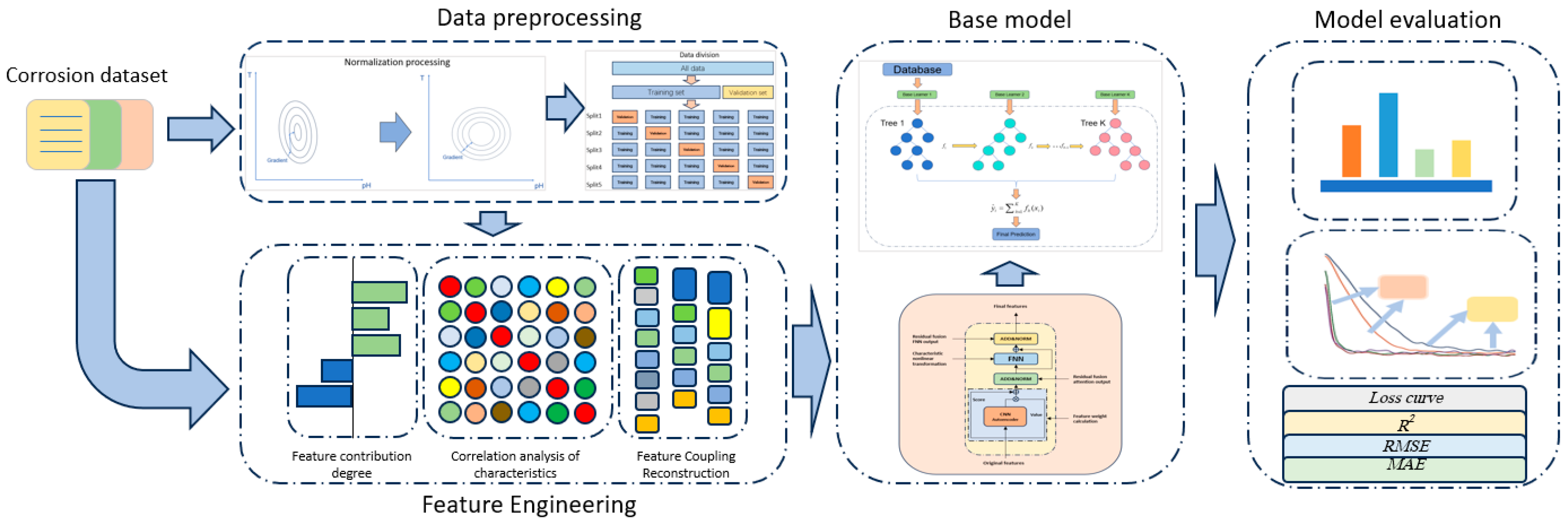
3.1. Data Source and Normalization Processing

Data was sourced from high-temperature and high-pressure weight-loss experiments on tubing corrosion. The dataset encompasses 8 feature variables and 1 target variable, totaling 220 data points. The experimental data structure is divided into influencing factors and outcomes. The selected influencing factors are: temperature (T), CO₂ partial pressure (PCO₂), H₂S partial pressure (PH₂S), N₂ partial pressure (PN₂), total pressure (PT), flow velocity (V), corrosion time (Time), and pH value (pH). The outcome is the corrosion rate. The corrosion subjects are three commonly used industrial metals: 2205DSS, N80, and CT80.

Table 1. Experimental corrosion rate data set.

Material	Temperature (°C)	CO2 Partial Pressure (MPa)	H2S Partial Pressure (MPa)	N2 Partial Pressure (MPa)	Total Pressure (MPa)	pH	Flow Velocity (m/s)	Corrosion Time (h)	Corrosion Rate
2205DSS	20	2	0	13	15	6	1	120	0.0058
2205DSS	40	2	0	13	15	6	1	120	0.0063
N80	40	1.5	0.6	12.9	15	5	1	72	0.0109
N80	100	1.5	0.9	12.6	10	3.9	1	72	1.6741
CT80	140	0	0	28.5	30	5	1	12	6.1388

shows partial examples from the raw corrosion rate dataset. Additionally, the input features in the current study are limited to specific factors currently available and do not yet cover other critical factors that may influence the internal corrosion rate of oil pipelines. In-depth exploration of the relevant influence mechanisms and multi-factor coupling effects still requires further research to supplement and refine.

Following the data processing methods outlined in Section 2.1, the raw data (which, coming from our weight-loss corrosion experiments, ideally have no missing or outlier values) underwent cleaning operations including missing value imputation and outlier removal. Subsequently, the Min-Max normalization method was applied to map all feature variable values to the [0, 1] range.

Table 2. Partial examples of the normalized data.

Material	Temperature (°C)	CO2 Partial Pressure (MPa)	H2S Partial Pressure (MPa)	N2 Partial Pressure (MPa)	Total Pressure (MPa)	pH	Flow Velocity (m/s)	Corrosion Time (h)	Corrosion Rate
2205DSS	0.16	0.387	0	0.126	0.1	0.395	0.33	0.7	0.00037
2205DSS	0.48	0.387	0	0.126	0.1	0.263	0.33	0.7	0.00102
N80	0.32	0.285	0.3	0.124	0.1	0.263	0.33	0.4	0.03287
N80	0.64	0.285	0.3	0.124	0.1	0.263	0.16	0.4	0.05233
CT80	0.96	0.261	0.128	0.423	0.4	0.131	0.33	0.025	0.71964

presents partial examples of the normalized dataset.

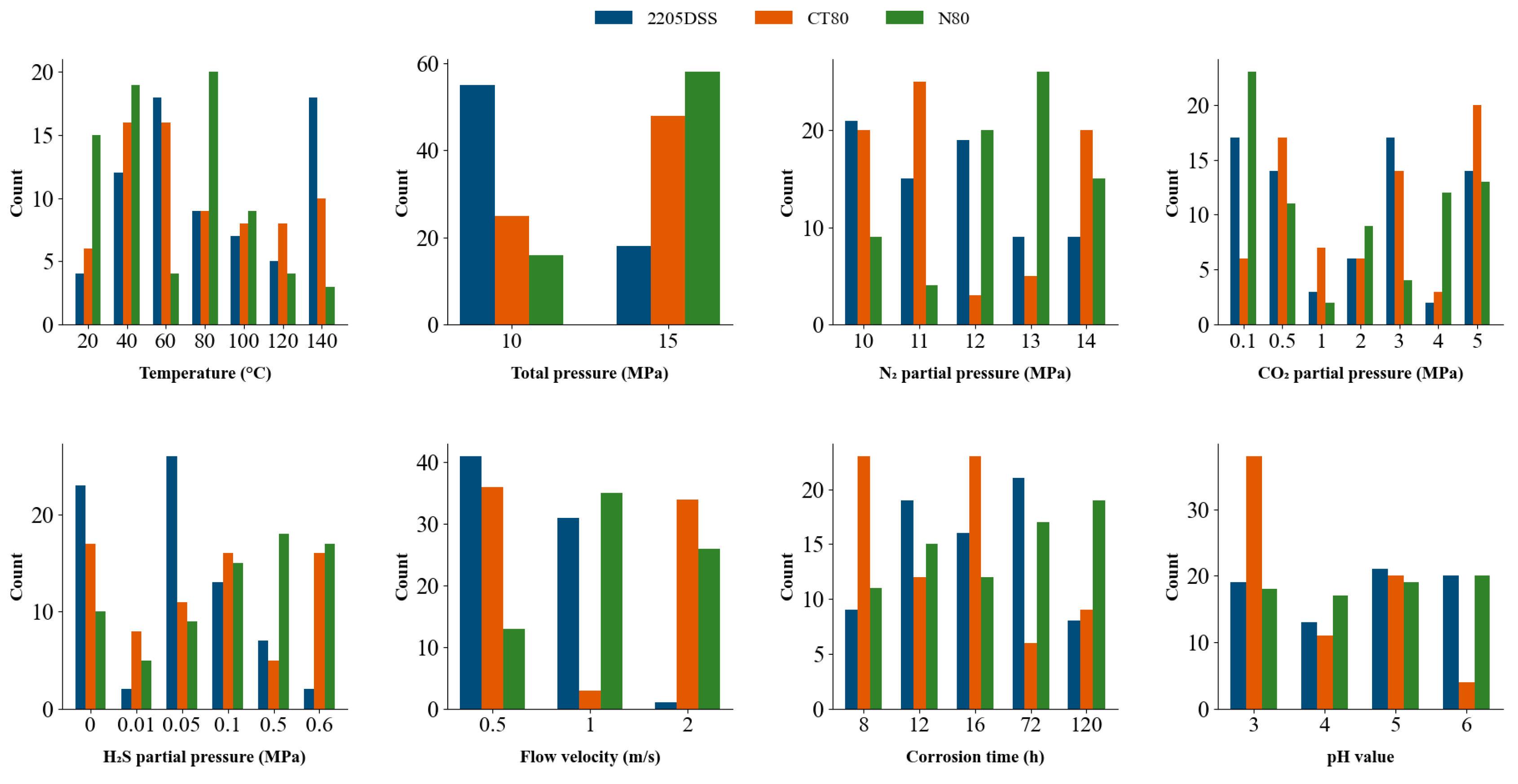
Data distribution histogram is shown in Figure 4 to more intuitively illustrate the coverage range and distribution of the features.

The normalized data were divided using five-fold cross-validation while being stratified by material type. By strictly maintaining the proportion of samples from different materials in each fold identical to the overall dataset, the material distribution characteristics of each fold were ensured to closely match the original data distribution. This approach avoided excessive concentration or absence of any single material type in a particular fold, thereby safeguarding the objectivity and reliability of the model’s prediction results.

3.2. Global Analysis of Features and Coupled Reconstruction

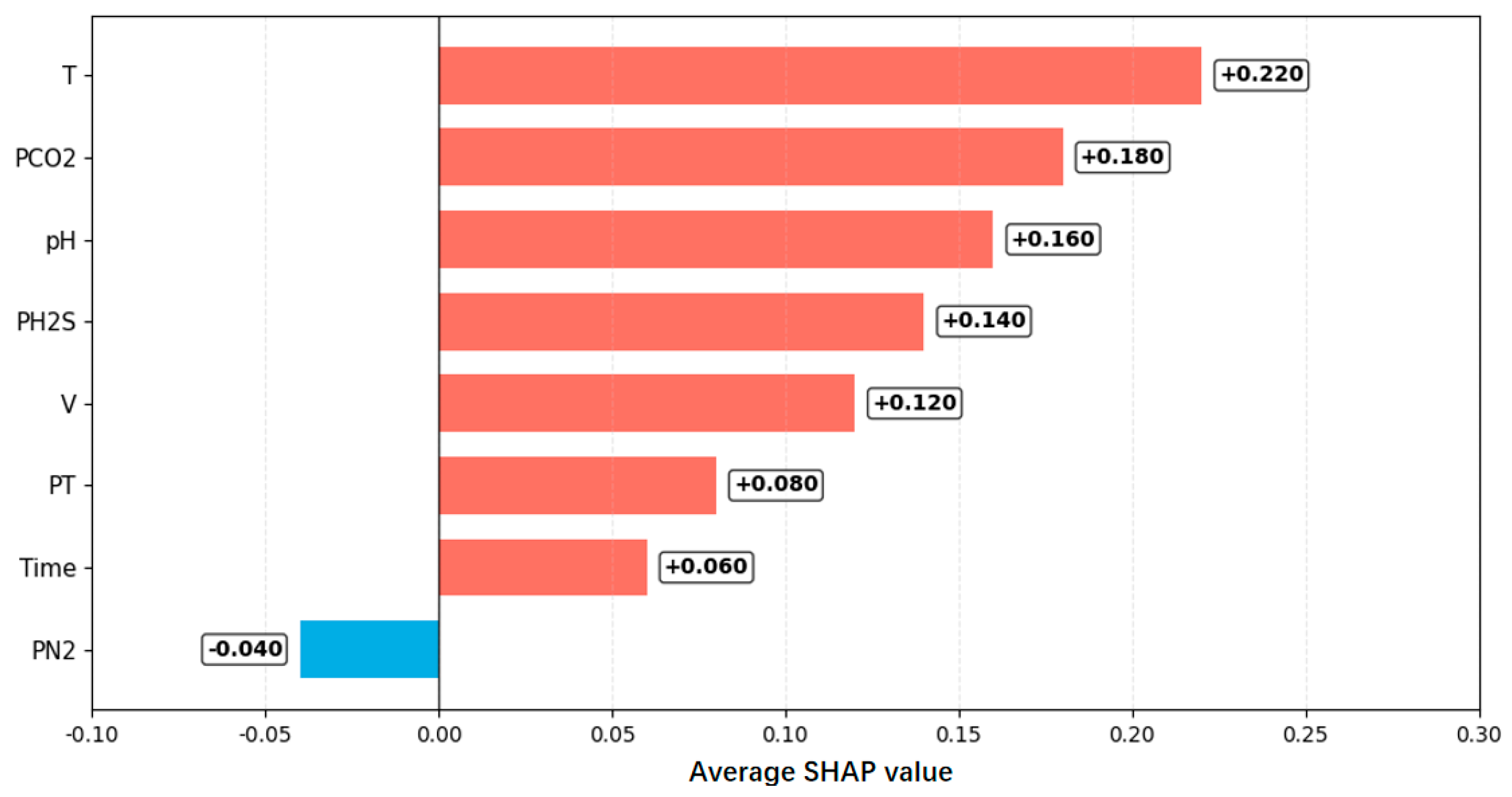
This study focuses on constructing a new dataset through feature coupling and weight reassignment to train and validate models, thereby revealing underlying feature interaction mechanisms. This section builds coupled features by integrating mathematical operations with corrosion domain knowledge, quantifying their synergistic influence beyond independent feature analysis. First, SHAP analysis is applied to the dataset, followed by normalization to obtain the average SHAP values for each independent feature. This enables analysis of their fundamental influence on corrosion rates and preliminary exploration of underlying physical mechanisms. A negative value for a feature indicates an inhibitory effect in the current sample, while a positive value signifies that the presence or intensity of that condition promotes the predicted outcome.

The horizontal bar chart in Figure 5 illustrates the contribution levels of each feature. Results indicate that temperature is the dominant factor controlling internal pipeline corrosion behavior; CO₂ partial pressure serves as the key driving force, ranking second; while pH and H₂S partial pressure is the third and fourth most significant factors. Other factors, such as flow velocity, total pressure, and time, exert relatively limited influence. This ranking reveals three core characteristics—temperature, CO₂ partial pressure, and pH—whose physical mechanisms are relatively well-established: temperature primarily governs reaction kinetics and protective film evolution; CO₂ partial pressure dominates cathodic depolarization reactions; and pH directly defines the corrosive intensity of the medium [37,38]. Notably, nitrogen, as an inert gas, exhibits corrosion-inhibiting effects by diluting the concentration of corrosive gases, thereby reducing their effective concentration at the metal surface [39].

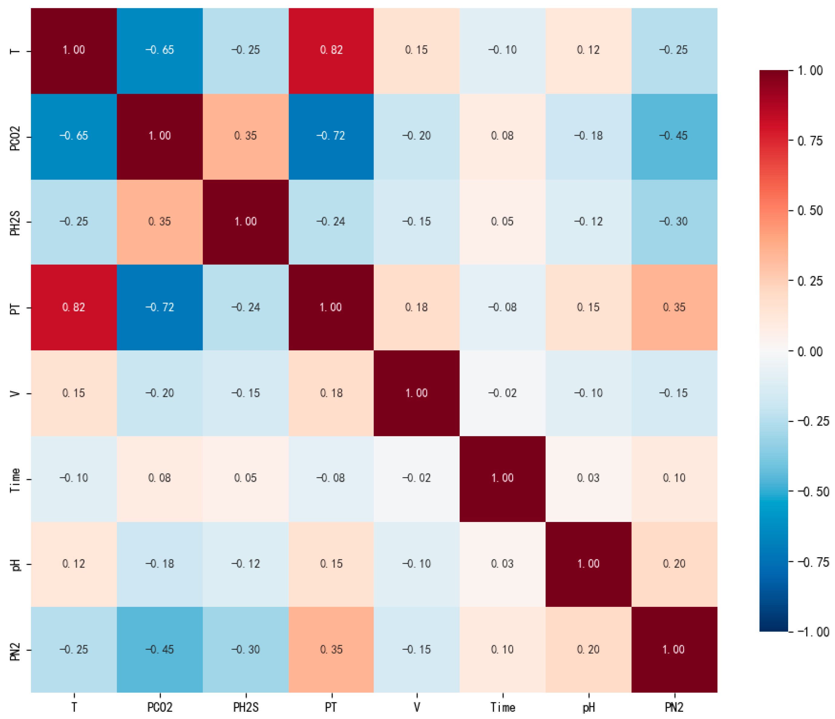
Correlation analysis was performed on all features to identify highly linearly correlated feature pairs, providing a basis for subsequent feature coupling. The Pearson correlation matrix in Figure 6 displays correlations among features, where numerical values represent correlation coefficients, positive/negative signs indicate directionality, and absolute values reflect linear relationship strength. Results show: Total pressure and CO₂ partial pressure exhibit a strong negative correlation with a coefficient of −0.72, further validating the mechanism of corrosion inhibition through nitrogen injection to increase system total pressure and dilute corrosive gases. Concurrently, CO₂ partial pressure and H₂S partial pressure—two critical corrosion parameters—show a moderate positive correlation, indicating they do not act independently in the corrosive environment but exhibit a degree of interdependence.

Building upon the correlations identified in the above analysis, this study next employs the SHAP-Sobol feature weighting method. By calculating the weights of individual features and their coupling terms, we quantify the relative contributions of independent effects and interaction effects in corrosion prediction. For the identified key feature pairs, this study selects the total pressure-temperature and CO₂ partial pressure-H₂S partial pressure feature sets for coupling and weight quantification analysis. This addresses two typical interaction scenarios: the environmental coupling of total pressure and temperature in actual pipeline service conditions, and the medium synergy between CO₂ partial pressure and H₂S partial pressure. The goal is to clarify the specific influence intensity of these core interaction terms on corrosion rates.

Table 3. Feature prediction weights before and after coupling.

Feature	Prediction Weight	Feature	Prediction Weight	Feature	Prediction Weight	Feature	Prediction Weight
T	0.3058	-	-	-	-	-	-
PCO2	0.2060	T-PT	0.5452	PCO2-PH2S	0.5171	T-PT	0.4017
PH2S	0.1726	PCO2	0.2181	T	0.3152
pH	0.1216	pH2S	0.1343	pH	0.1166	PCO2-PH2S	0.3839
Time	0.0949	pH	0.0984	Time	0.0765	pH	0.1383
V	0.0534	Time	0.0762	V	0.0656	Time	0.0897
PT	0.0345	V	0.0635	PT	0.0545	V	0.0591
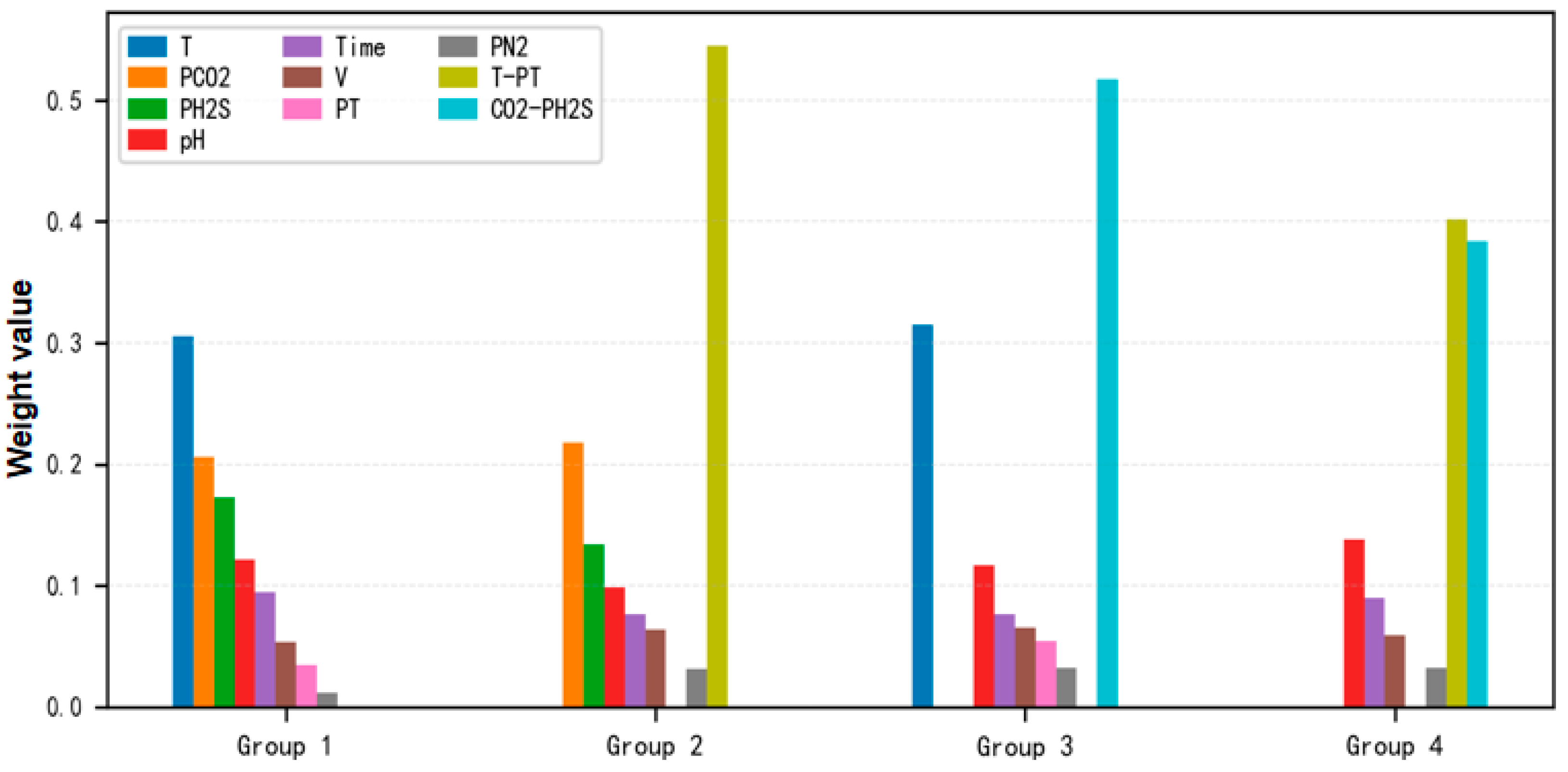
PN2	0.0112	PN2	0.0313	PN2	0.0321	PN2	0.0323

presents the feature prediction weights before and after coupling, while Figure 7 illustrates the comparison between independent and coupled feature prediction weights. Among them, Group 1 contains only the original independent features (no coupling terms); Group 2 introduces the temperature-total pressure (T-TP) interaction term based on the original features; Group 3 introduces the CO₂-H₂S partial pressure (PCO₂-PH₂S) interaction term; and Group 4 includes both interaction terms.

A comparative analysis reveals distinct feature prediction weights across each group. The first group exhibits a total feature prediction weight of 1, as it incorporates only independent features without accounting for coupling effects between them. In contrast, the subsequent three groups all yield total weights exceeding 1. This occurs because within the SHAP-Sobol analytical framework, the method independently quantifies two distinct contributions: First, the marginal importance of each feature. Second, the synergistic contribution from feature coupling effects. These contributions neither cancel each other out nor overlap; instead, they manifest as a complex, multi-factor logical superposition characteristic of complex systems. When coupling effects generate additional explanatory power, the total weight may slightly exceed 1. It should be noted that weight normalization is not performed here. The purpose is to preserve the original magnitude of the coupled contribution, facilitating an intuitive comparison of the weight jump before and after coupling. Forced normalization would mask the true degree of enhancement of the coupled term, thereby reducing interpretability. Subsequently, these prediction weights will be embedded into the established model architecture. By comparing prediction results before and after feature coupling, we will intuitively reveal the patterns of how coupling effects influence corrosion prediction.

3.3. Model Hyperparameter Optimization

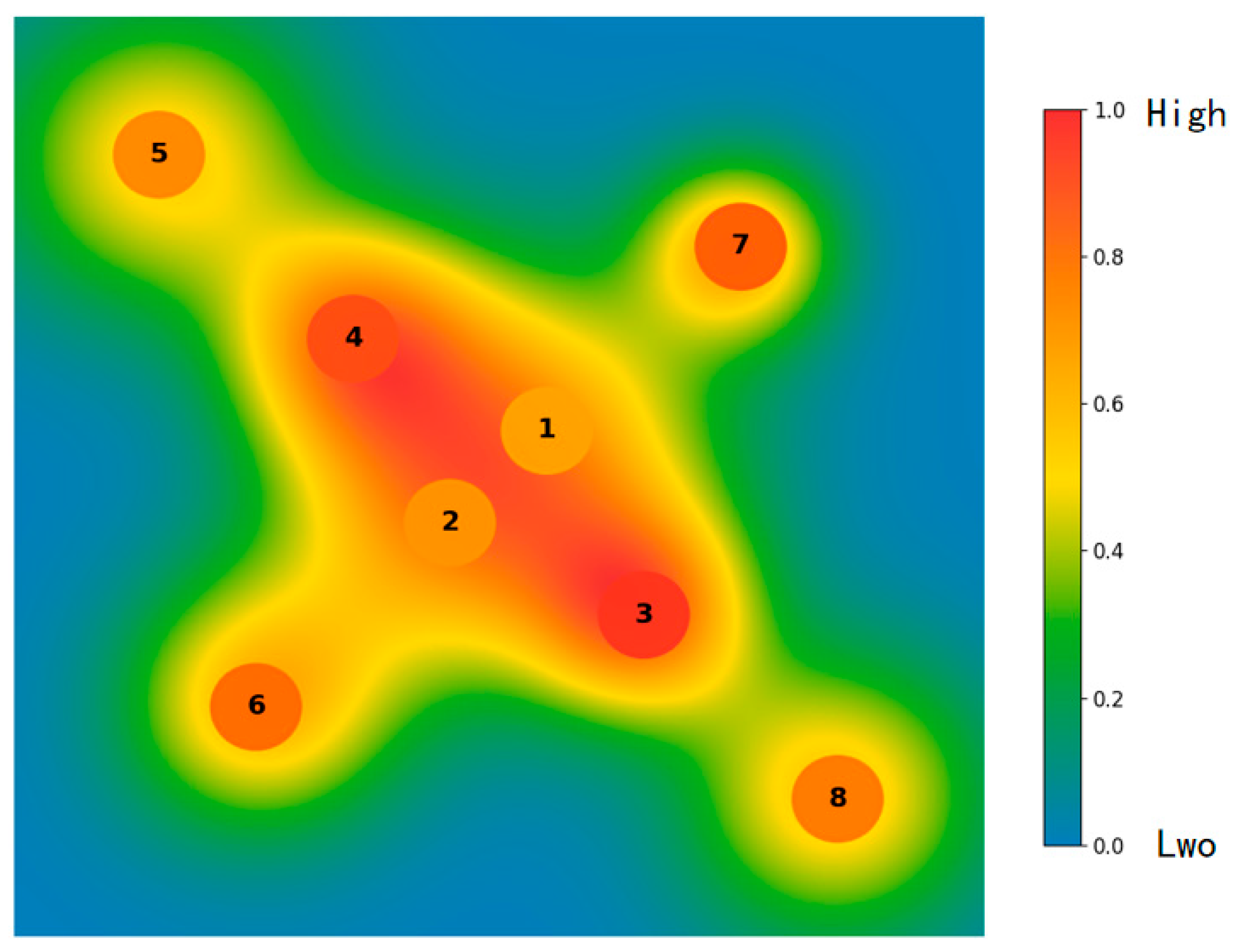
Before embedding feature prediction weights into the model, it is essential to systematically identify the optimal hyperparameter combination. This ensures subsequent predictions utilize a consistent model architecture, thereby attributing all result variations solely to the introduction of the feature weight quantization strategy and avoiding interference with hyperparameter tuning. Employing Bayesian optimization through multiple iterative rounds, we ultimately identified eight high-performance model configurations (Figure 8). The distribution of models within the parameter space exhibits distinct performance gradient characteristics, where color intensity correlates positively with prediction accuracy—darker regions indicating superior model performance under corresponding parameter settings. This optimization outcome provides reliable candidates for the final determination of hyperparameter combinations. Building upon this foundation, we will comprehensively evaluate each model’s generalization capability and stability through convergence curves of training and validation losses, thereby establishing a more holistic basis for finalizing model hyperparameter configurations. During the model testing phase, each configuration was trained and validated using identical datasets, including uniform training and validation set partitions, ensuring comparability among models.

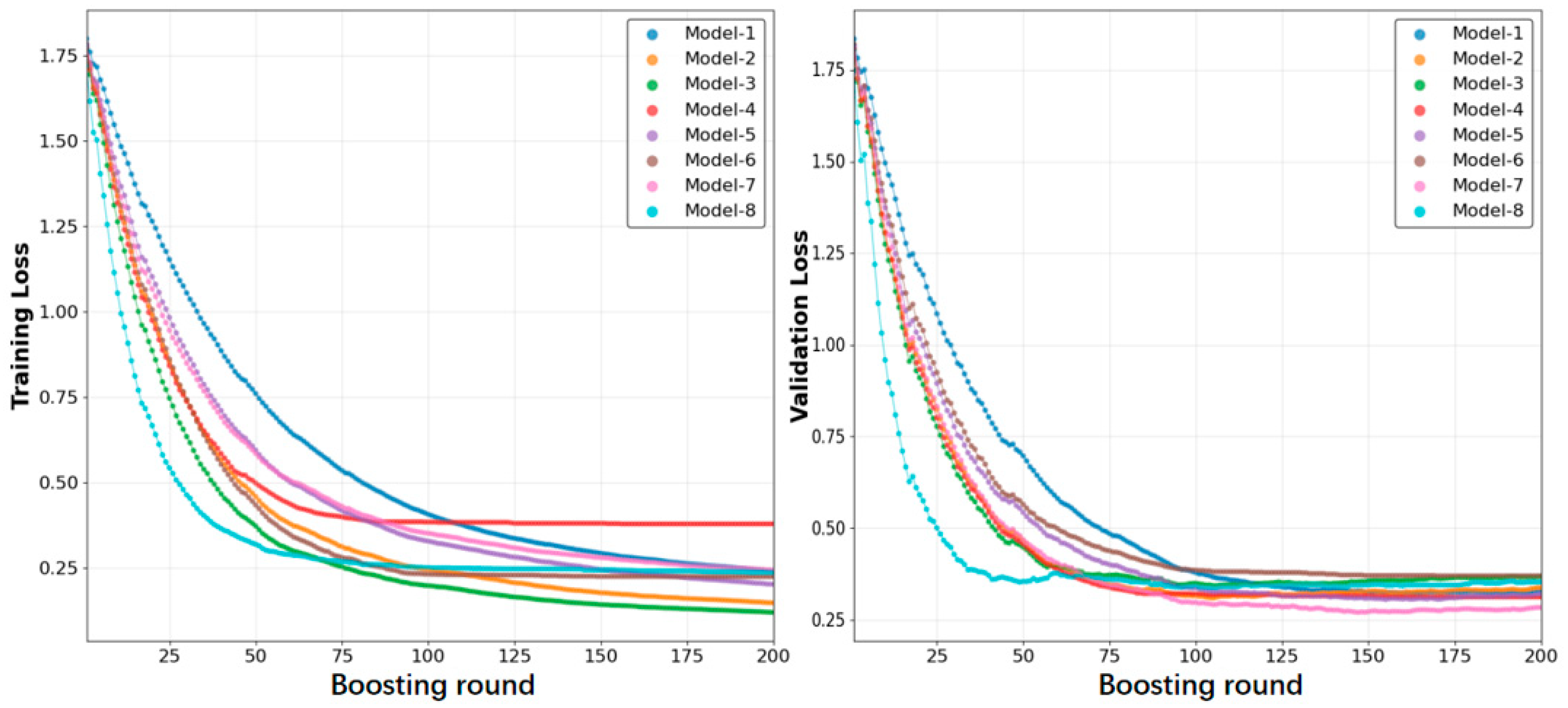
The loss function employed is the Mean Squared Error (MSE). The resulting loss curves are shown in Figure 9. The testing process is strictly confined to 200 boosting rounds, with complete records of training and validation loss variations. Dense scatter plots visually display the loss curve trajectories of each model throughout the training cycle, clearly illustrating the convergence characteristics and overfitting tendencies under different hyperparameter configurations.

$$MSE={\displaystyle \frac{1}{n}}{\displaystyle {\sum }_{i=1}^n{\left(x_i-{\widehat{x}}_i\right)}^2}$$

(17)

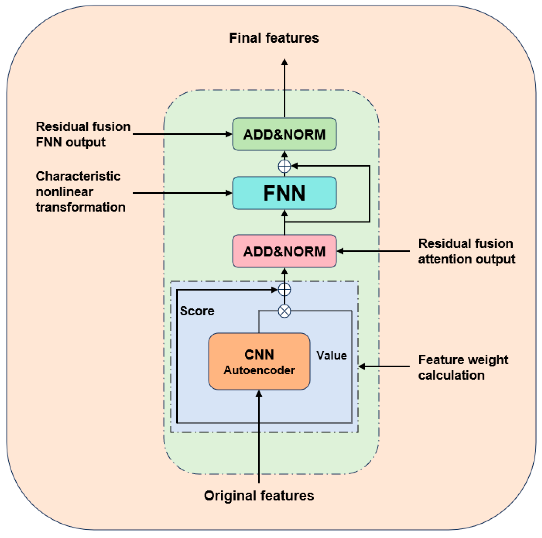
Based on the loss curve analysis, all eight models demonstrated excellent convergence characteristics. The training and validation losses good performance for all models achieved rapid and stable decreases within 200 training boosting rounds, with no noticeable signs of overfitting. This synchronized behavior indicates the models possess satisfactory generalization within the tested dataset. Notably, Model 3 achieved optimal performance on the validation set, with a smooth and continuously decreasing validation loss curve, demonstrating excellent prediction accuracy and stability. Although Model 8 performed slightly less well, its rapid convergence capability in the early stages remains significant for scenarios requiring swift model validation. Minor fluctuations observed in some models during late training stages may indicate optimization instability. Although overall model performance is satisfactory, robustness under more extreme operating conditions requires further validation. After a comprehensive evaluation, this study adopts the hyperparameter configuration of Model 3 for subsequent prediction tasks. The remaining two models also underwent the same process to select their best configurations, and all subsequent comparative analyses will uniformly use these optimally configured models. The specific configurations are shown in

Table 4. Configuration of model hyperparameters.

Prediction Model	Hyperparameter	Configuration
XGBoost	Number of trees	180
	Max depth	3
	Learning rate	0.1
	Subsample ratio	0.8
	Column sample ratio	0.9
RF	Number of trees	180
	Max depth	3
	Max features	2
	Min samples per leaf	3
GPR	Kernel type	Matérn (ν = 1.5)
	Length scale	0.8
	Noise variance	0.03

.

3.4. Analysis of Prediction Results

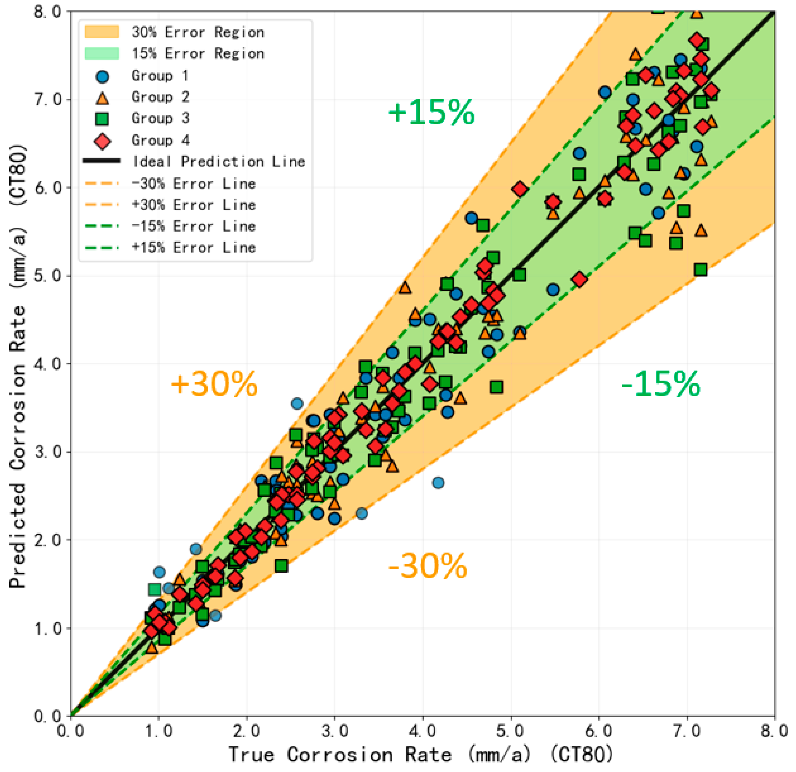
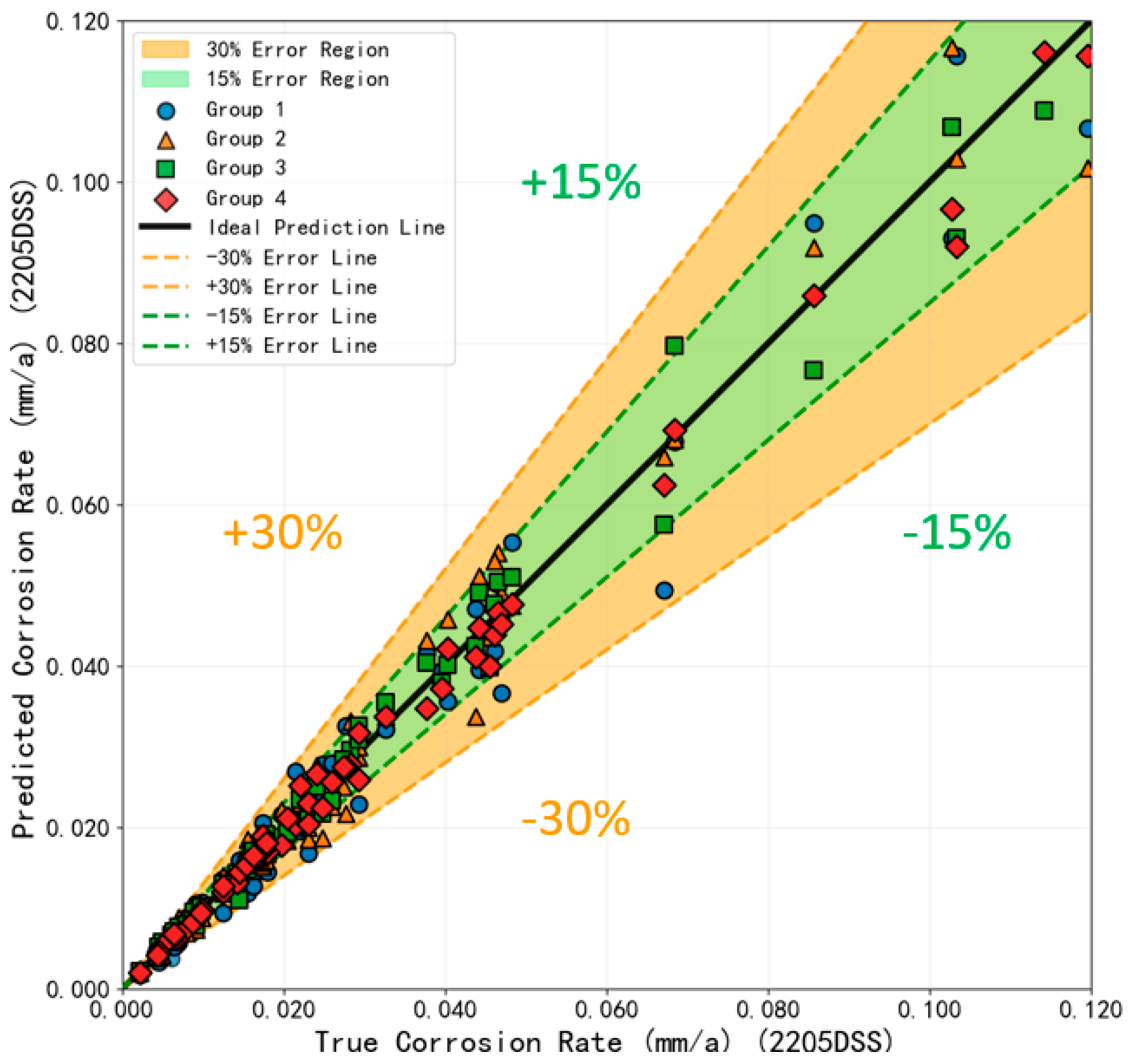
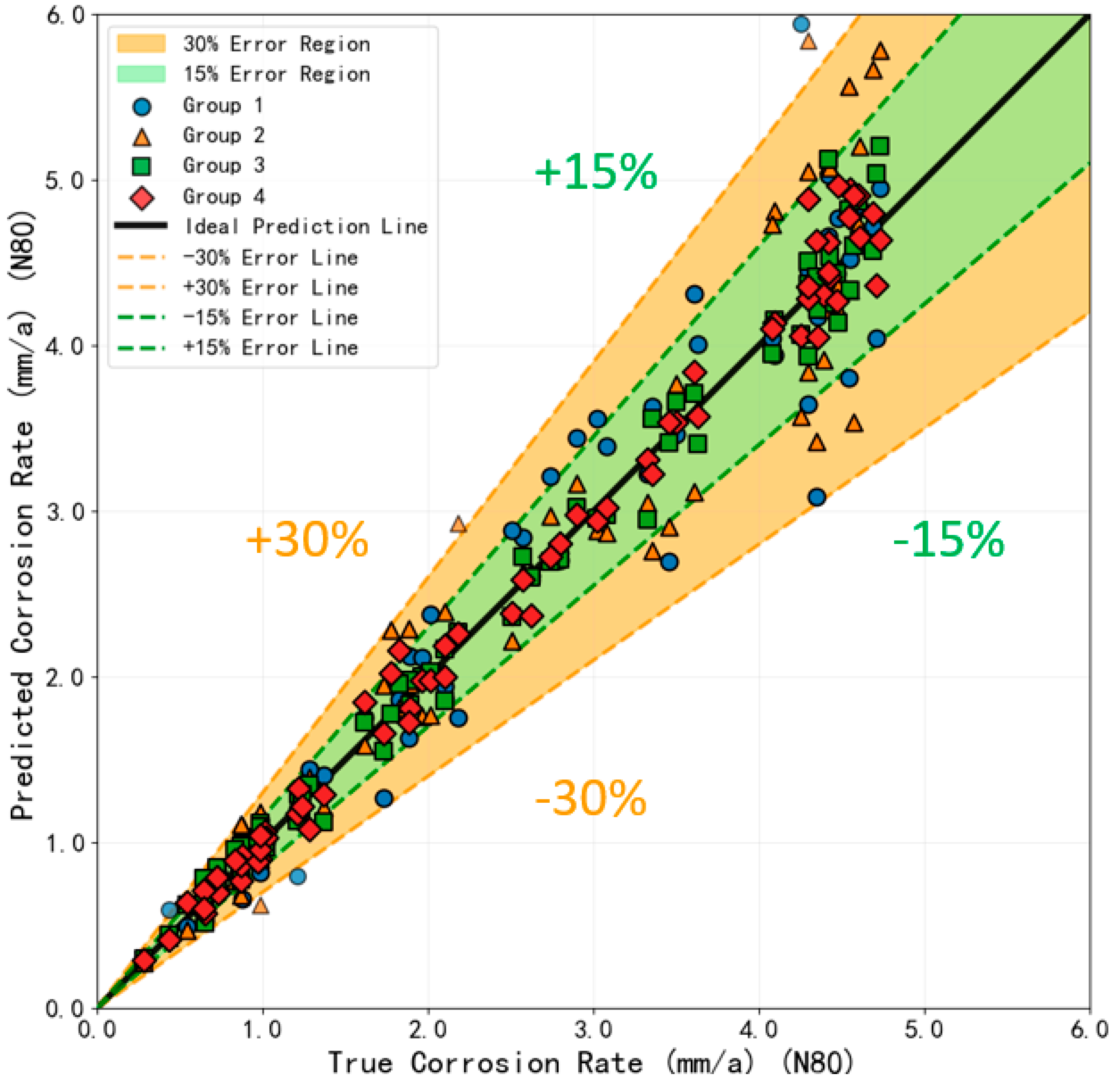
The feature prediction weights from each group were embedded into the selected model framework to predict and analyze the corrosion rates of three tubular steel grades. Results shown in Figure 10, Figure 11 and Figure 12 demonstrate the performance of models incorporating different feature combinations in predicting corrosion rates for the three tubing materials. The error distribution of prediction results reveals significant differences in sensitivity to feature groups across materials due to variations in material properties and corrosion mechanisms. For the 2205DSS duplex stainless steel, the prediction accuracy improved after introducing the gas interaction term, with a noticeable increase in the proportion of data points falling within the 15% error band. This result suggests that even for this corrosion-resistant duplex stainless steel, the synergistic effect of CO₂ and H₂S still affects the stability of its passive film, further indicating that this coupled feature is key to controlling its corrosion rate. According to the SHAP analysis, the CO₂-H₂S interaction term has a contribution weight of 0.5171. The model infers that when the partial pressure ratio of the two gases increases, the passive film stability decreases, leading to a higher predicted corrosion rate; conversely, a lower rate is predicted. This behavior is consistent with changes in the film breakdown potential observed in electrochemical tests.

CT80 carbon steel exhibits a stronger dependence on the T-PT coupling feature. After introducing this feature combination, the model prediction error significantly decreases and the high-accuracy prediction points become more concentrated, reflecting the important role of temperature and pressure in the corrosion behavior of this material. The model assigns the highest weight (0.5452) to the T-PT coupling feature, and the predictions show that under high-temperature and high-pressure conditions the corrosion rate increases sharply. The interpretability analysis indicates that temperature accelerates the reaction kinetics while pressure increases gas solubility, jointly promoting corrosion; therefore, temperature control should be prioritized in the field. It is worth noting that although characteristics such as time and flow velocity appear in all combinations, the introduction of the T-PT coupling term also enhances the synergistic representation capability of these fundamental parameters.

The predicted corrosion rate results for N80 steel show a distribution distinct from those of CT80 and 2205DSS, with the prediction accuracy strongly depending on the interaction of corrosive gases. Specifically, in the low-to-medium corrosion rate region (<4.0 mm/a), the model relies mainly on the CO₂-H₂S interaction term for prediction, and the predicted points lie densely near the ideal line, agreeing well with the measured values. However, when the actual corrosion rate exceeds 4.0 mm/a, the predicted points begin to deviate significantly from the ideal line, forming a distinct divergence zone. This phenomenon suggests that as the corrosion intensity increases, the corrosion mechanism of N80 steel may gradually shift from a CO₂-H₂S interaction-dominated mode to a composite mechanism governed by more localized factors such as pitting and flow field disturbance. The interpretability analysis indicates that the divergence at high corrosion rates stems from the absence of features describing corrosion product film rupture in the current model; therefore, relevant factors should be introduced in the future to improve prediction reliability in the high-corrosion-rate range.

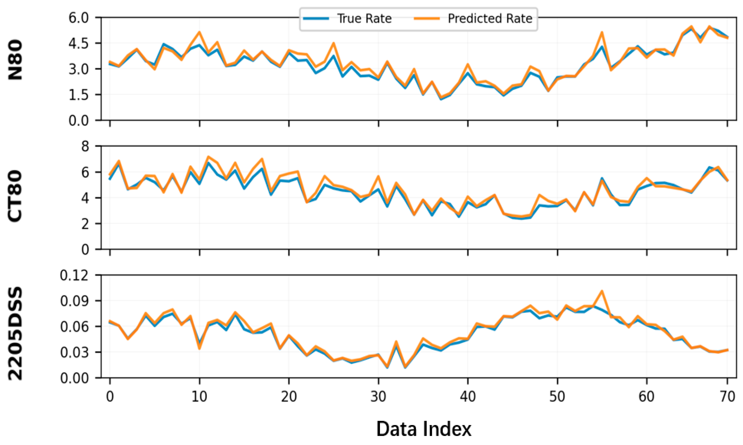
Figure 13 displays the comparison profiles between predicted and actual values for the three materials. The predicted values uniformly adopt the model prediction results embedded with the fourth set of feature prediction weights. Overall, the model demonstrates good predictive accuracy on the test set in predicting corrosion rates for all three materials. The predicted curves for N80 and CT80 exhibit slight fluctuations relative to the actual curves, while the predicted curve for 2205DSS shows a smoother, more stable trend. This variation correlates positively with the inherent complexity of corrosion behavior and data variability for each material. Collectively, these findings demonstrate the model’s ability to effectively capture the distinct corrosion characteristics of different materials, with prediction results possessing potential engineering reference value.

Table 5. Comparison of prediction performance metrics among models with different feature configurations.

Material	Feature Set	R2	RMSE	MAE
N80	Group 1	0.900	0.45	0.32
N80	Group 2	0.920	0.38	0.27
N80	Group 3	0.960	0.28	0.19
N80	Group 4	0.980	0.18	0.12
CT80	Group 1	0.890	0.65	0.48
CT80	Group 2	0.940	0.42	0.31
CT80	Group 3	0.930	0.48	0.35
CT80	Group 4	0.970	0.30	0.22
2205DSS	Group 1	0.870	0.018	0.014
2205DSS	Group 2	0.900	0.015	0.013
2205DSS	Group 3	0.940	0.014	0.012
2205DSS	Group 4	0.980	0.013	0.010

compares the predictive performance metrics of models with different feature configurations. Results show the coefficient of determination R² reached an outstanding maximum of 0.98, indicating the model possesses strong predictive capability for oil pipe corrosion rates without overfitting. Regarding error analysis, both MAE and RMSE metrics remain within ideal ranges. The prediction error for 2205DSS steel is the lowest, while those for CT80 and N80 steels are slightly higher but still within acceptable limits. Overall results demonstrate that the constructed model possesses excellent generalization capability and engineering practicality, providing reliable data support and decision-making basis for tubing material selection and corrosion protection.

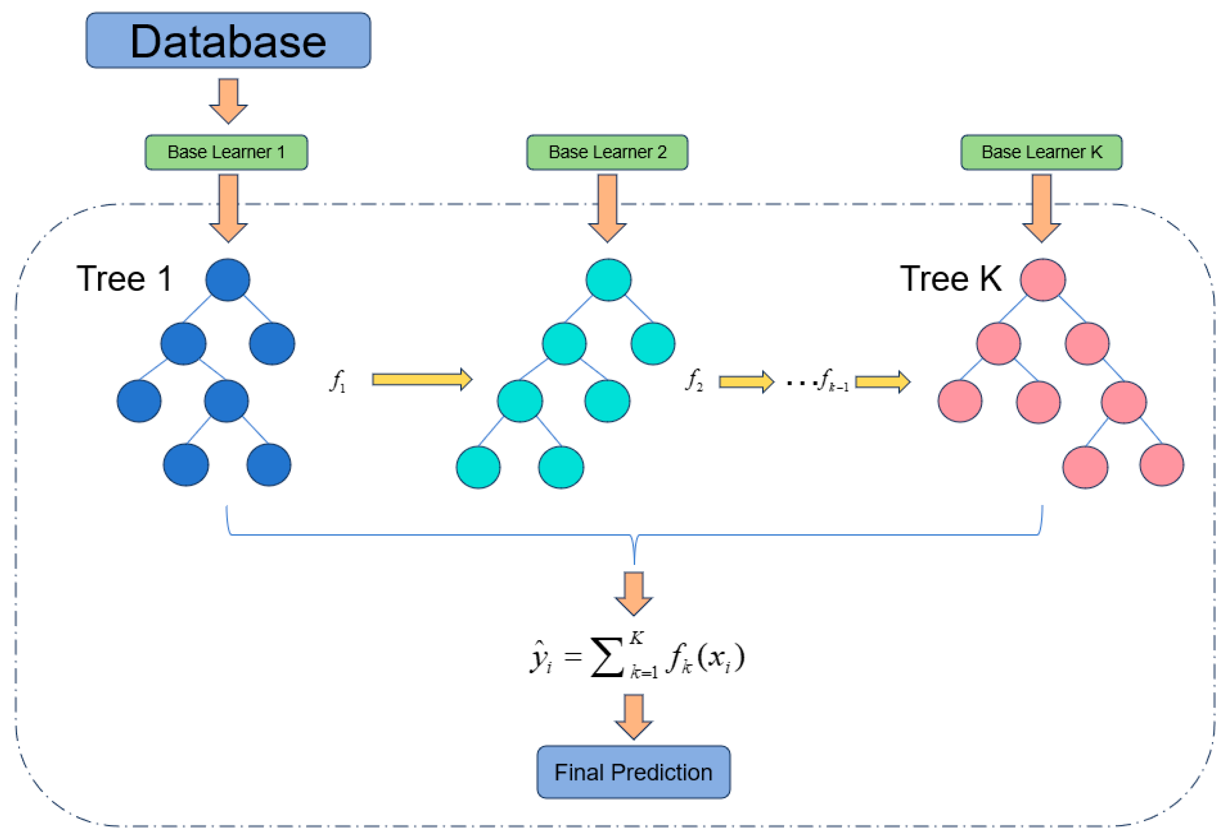
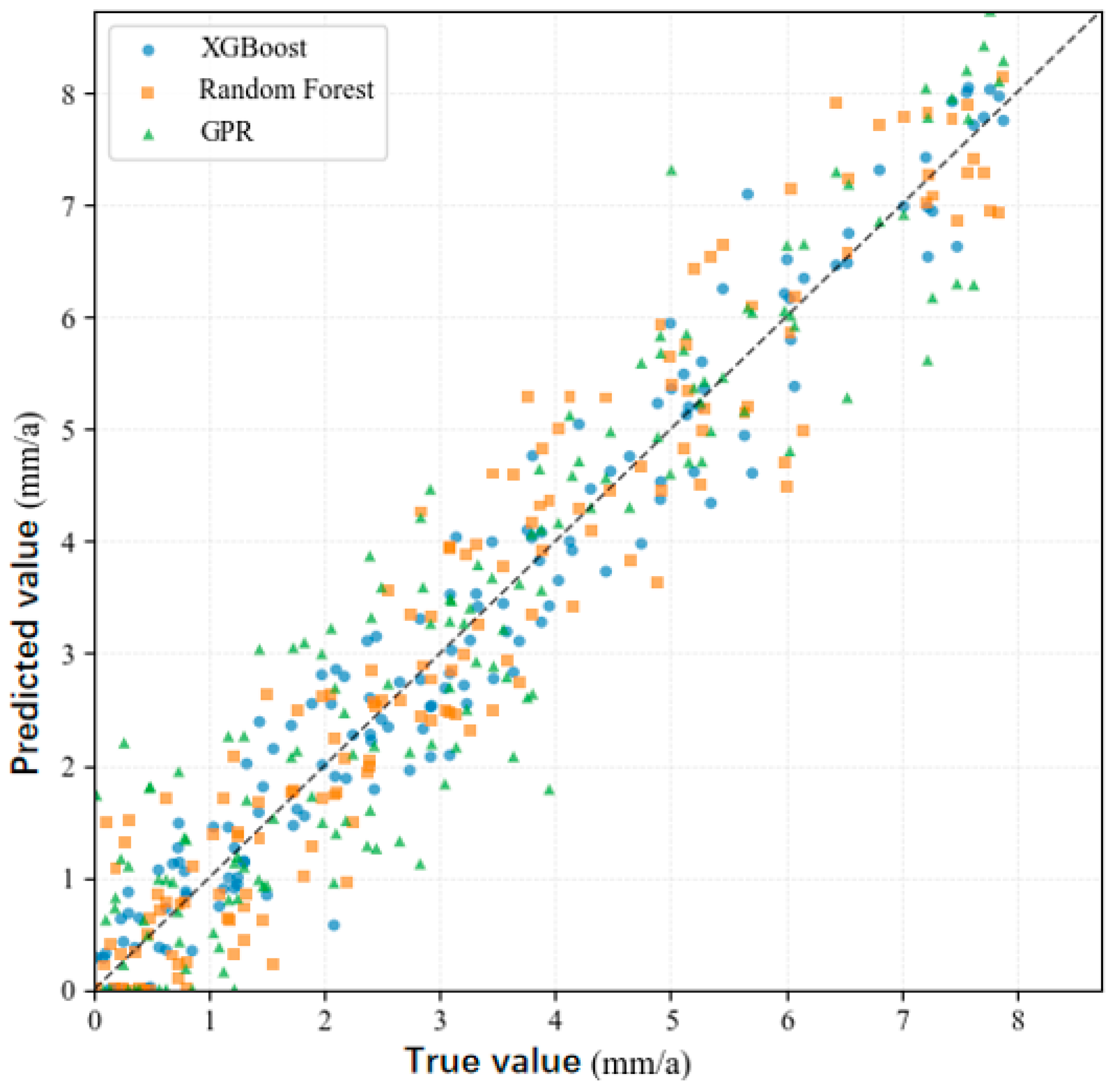
For the remaining two prediction models, this study compares their predictive performance on the overall dataset with that of the core XGBoost model. Through the visualization of the prediction results of each model on the same test set, as shown in Figure 14, the scatter distribution of the predicted values versus the true values for the three models is presented.

As can be observed from the figure, the prediction points of XGBoost are the most concentrated, basically distributed along the diagonal line within the corrosion rate range of 0–5 mm/a, indicating that its prediction error is small and uniformly distributed. The prediction points of Random Forest show some dispersion in the low-value range (0–2 mm/a), but still maintain a good tracking trend in the high-value range. The prediction points of Gaussian Process Regression (GPR) are relatively more dispersed, with noticeable fluctuations especially in the intermediate value region, yet it still effectively captures the overall trend of corrosion rate variation. When further optimizing the prediction model, one may consider introducing more discriminative feature combinations tailored for high corrosion rate conditions to enhance the model’s adaptability across the full rate range and its engineering guidance value.

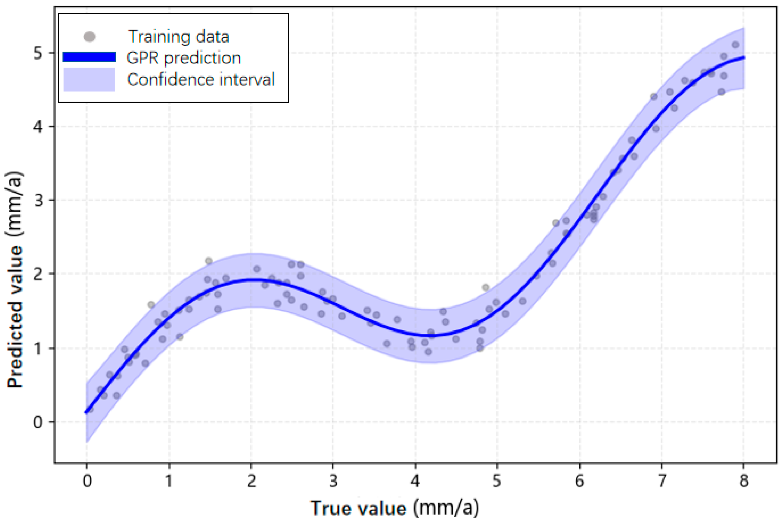
It is worth noting that the confidence interval output capability of GPR gives it unique value in corrosion risk early warning. As shown in Figure 15, GPR not only provides point estimates on the test set but also supplies prediction confidence intervals that vary with features. In regions where data are sparse or operating conditions are abnormal (e.g., the right end of the figure), the confidence interval widens significantly, indicating reduced reliability of the model prediction, which should be carefully interpreted in conjunction with field experience. In contrast, XGBoost and Random Forest only output single predicted values and cannot quantify such uncertainty, making GPR an important tool for corrosion risk assessment.

Table 6. Three model prediction performance indicators.

Model	R2	RMSE	MAE
XGBoost	0.96	0.28	0.19
RF	0.92	0.45	0.32
GPR	0.88	0.48	0.35

presents the comparison results of various evaluation indicators for the prediction performance of the three machine learning models.

Table 7. The time spent on training and validating the three models.

Model	Training Time (s)	Validating Time (s)
RF	0.1307	0.017096
XGBoost	0.8952	0.002005
GPR	1.1819	0.001000

shows the time spent on training and validation for the three models.

Overall, the XGBoost model demonstrates the best accuracy in corrosion rate prediction, with its coefficient of determination (R²), root mean square error (RMSE), and mean absolute error (MAE) all significantly outperforming those of the RF and GPR models. Although the training time of the XGBoost model is slightly longer than that of the RF and GPR models, its prediction speed is extremely fast, enabling rapid and accurate identification of abnormal fluctuations in corrosion rate based on real-time operating parameters, making it suitable for deployment in online monitoring systems. The RF model has the fastest training speed but slightly lower prediction accuracy, making it suitable for rapid modeling or preliminary exploration scenarios. Although the GPR model lacks sufficient accuracy, it provides uncertainty intervals for predictions and can serve as a supplementary tool for risk assessment and decision support. In practical applications, the model can be flexibly selected according to requirements for accuracy, modeling speed, and uncertainty evaluation.

3.5. Discussion on the Applicability and Limitations of This Study

The model developed in this study applies to three pipe materials (2205DSS, CT80, N80) and provides corrosion rate predictions that combine accuracy and interpretability under the tested complex operating conditions. For other types of corrosion behavior, the established comprehensive prediction process may remain applicable, provided that relevant feature data reflecting their mechanisms can be obtained. This offers preliminary evidence to help identify key corrosion factors and formulate control strategies, suggesting potential for extension.

However, this study has several limitations. First, model training relies on existing feature variables and does not yet encompass other potential influencing factors; therefore, its generalization capability under novel or extreme conditions requires further validation, preferably with independent datasets. Second, the model’s inclusion of an attention mechanism and interpretability analysis modules results in higher computational complexity compared to traditional prediction methods. Finally, differences in feature responses across materials indicate that constructing a fully universal prediction model remains challenging, and adaptation to specific material systems is necessary.

Within the current dataset, the proposed interpretable corrosion prediction model supports the formulation of pipeline integrity management strategies, potentially enabling a shift from reactive maintenance to proactive early warning. This approach may enhance system safety and environmental risk prevention capabilities while reducing operational costs, although these benefits have not yet been demonstrated in live field applications. Future work will continue validating and optimizing this method across broader material systems and corrosion scenarios, further integrating mechanistic models with field data to build a more robust and efficient corrosion prediction platform, with the ultimate goal of achieving wider practical applicability.

4. Conclusions

This study developed an ensemble prediction model based on CASA-XGBoost to forecast corrosion rates of oil pipelines under multi-factor coupled environments using experimental and field data. The SHAP-Sobol feature weighting method was employed to assess input feature importance, analyze independent and coupled contributions, and establish an interpretable prediction framework. This framework not only reveals the influence mechanisms of various environmental factors on corrosion rates but also provides an intuitive and reliable corrosion prediction tool for engineering practice. Key conclusions are summarized as follows:

(1)

Through SHAP-Sobol weight quantification analysis, temperature (T) was identified as the primary factor influencing corrosion rate, followed by the CO₂ partial pressure and pH value. Additionally, the coupled effect of temperature-total pressure (T-PT) and CO₂-H₂S partial pressure (PCO₂-PH₂S) was found to significantly impact corrosion behavior across different steel grades.

(2)

Compared with RF and GPR, the XGBoost model demonstrated superior prediction performance for three representative tubular steels (2205DSS, CT80, N80). Following feature coupling reconstruction, the model achieved a maximum R² of 0.98 a significantly reduced MAE and RMSE, outperforming both RF (R² = 0.92) and GPR (R² = 0.88).

(3)

The model exhibits distinct feature sensitivities across materials: 2205DSS is highly influenced by gas interactions, CT80 is more sensitive to temperature–pressure coupling, and N80 shows reduced predictive performance at high corrosion rates. This indicates that feature adaptation and model optimization tailored to material properties are essential for corrosion prediction.

In summary, the interpretable CASA-XGBoost ensemble prediction model established in this study achieves high-precision, explainable forecasting of tubing corrosion rates under multi-factor coupling conditions, offering practical engineering value for tubing integrity management and corrosion protection decision-making.