A Short-Term Wind Power Prediction Method Based on Multi-Model Fusion with an Improved Gray Wolf Optimization Algorithm

Abstract

In the current energy context, enhancing the precision of wind power prediction serves as a key enabler for the stable development of the power grid. In the existing wind power prediction models, there are often problems of modal aliasing and noise residue, or the prediction accuracy of the model is not high. In an effort to solve the problem of short-term wind power forecasting, a wind power series decomposition and reconstruction method based on improved complete ensemble empirical mode decomposition with adaptive noise-variational modal decomposition (ICEEMDAN-VMD) secondary decomposition is proposed. Using ICEEMDAN, wind power data (wind direction, wind speed, temperature, humidity, air pressure, etc.) is decomposed into several IMF sub-series, and these IMF sub-series are categorized into three different frequency components by combining sample entropy, Q statistics and sequence frequency. Secondly, the gray wolf optimization (GWO) is improved by using the empirical exchange strategy (EES), and the optimization performance of the EES-GWO proposed in this paper is verified by using 10 test functions. Finally, the EES-GWO-convolutional neural network–bidirectional gated recurrent unit–global attention (EES-GWO-CNN-BiGRU–Global attention) high-frequency component prediction model is constructed. Finally, we employ the XGBoost model to forecast the mid- and low-frequency components, thereby generating the corresponding forecasting results. The support vector machine (SVM) model nonlinearly integrates all the forecasting results to produce the final forecasting results. Through example analysis and comparison, the performance of the proposed model is verified from two perspectives.

1. Introduction

Since the Industrial Revolution, the large-scale consumption of non-renewable energy resources represented by coal, oil and natural gas has triggered the triple challenge of climate crisis, environmental pollution and resource depletion. To solve these difficulties, the global consensus is promoting the transformation of the energy mix from high-carbon to low-carbon and even zero-carbon [1]. Renewable energy, represented by wind energy, has become one of the core paths to achieving the “dual carbon” goal and ensuring energy security and sustainable development due to its clean, renewable, and near-unlimited reserves [2,3].

Against this background, wind power prediction technology has emerged. Accurate wind power prediction can provide grid dispatch departments with reliable information about the power generation capacity of wind farms for a future period.

The previous wind power forecasting methods were mainly based on physical modeling and traditional statistical methods. For example, Chang et al. presented a hybrid predictive framework that first adjusted the raw numerical weather prediction (NWP) wind speed forecasts and then filtered out redundant NWP information through a multiscale deep learning regressor. Facing the difficulties of long-term wind power prediction, the accuracy of long-term forecasting has been effectively improved, and the research ideas and application value are more prominent. However, the model structure is complex and the computational cost is high [4]. Zhang et al. first outlined three representations of wind power uncertainty, then reviewed the corresponding modeling techniques. Finally, they synthesized the key requirements for uncertainty prediction and a general evaluation framework [5]. Kenmoé et al. evaluated six mainstream wind speed forecasting engines that spanned statistical and physical paradigms. On the statistical side, a single static neural network, a single dynamic neural network and two hybrid neural network architectures were compared with autoregressive integrated moving average (ARIMA) for multi-step-ahead prediction. Multi-step advanced wind speed prediction is realized by comparing multiple models and is used for wind turbine output estimation, but only traditional prediction models are used for comparison, and no advanced deep learning methods are introduced, and the prediction accuracy is limited [6].

In recent years, technologies have experienced explosive growth, driving widespread adoption of data-driven approaches—most notably temporal convolutional networks (TCNs), long short-term memory (LSTM) networks and other methods—for wind power prediction. Common single-model methods mainly include support vector machines (SVMs) [7], convolutional neural networks (CNNs) [8,9], LSTM [10], XGBoost [11,12], etc. These methods effectively overcome the limitations of traditional physical modeling approaches and greatly improve prediction accuracy and model robustness. Wang et al. constructed a wind power-forecasting engine that married TCN with the informer architecture. To curb information overload, a maximal-information-coefficient (MIC) filter first retained only the most relevant predictors; dynamic-time-warping (DTW) then set the optimal history length for past-power inputs. However, the model structure is relatively complex, the training and calculation cost is high, and the robustness and actual deployment applicability of the model need to be improved [13]. Reference [14] presented a hybrid wind power predictor that coupled complete ensemble empirical mode decomposition (CEEMD) with a whale optimization-augmented kernel extreme learning machine (WOA-KELM). The components obtained by CEEMD were then forecast by a KELM whose kernel parameters and bias were finetuned by WOA. The resulting component-wise predictions were finally summed to yield the aggregated wind power estimate.

Single models, however, often suffer from high prediction errors, limiting their practical deployment. Combined models further improve prediction accuracy by leveraging the advantages of other algorithms in data feature processing and prediction performance, CEEMDAN, attention mechanisms, etc., and are therefore widely adopted across diverse time series forecasting tasks. Reference [15] introduced a hybrid deep learning wind speed predictor that married the empirical wavelet transform (EWT) with two recurrent neural architectures. EWT first split the raw series into a bank of sublayers; LSTM networks forecast the low-frequency components, while Elman recurrent networks dealt with the high-frequency ones. Eleven competing models were benchmarked to compare the genuine skill of the proposed framework. Reference [16] introduced a forecasting method that combined CEEMDAN with an LSTM network, whose hyperparameters were further tuned by an improved whale optimization algorithm (IWOA). Reference [17] presented a multi-step interval forecasting approach that integrated CEEMDAN-Fuzzy information granulation (CEEMDAN-FIG) with a CNN–bidirectional long short-term memory (CNN-BiLSTM) network. Hou et al. presented a wind power predictor that synergized attention, convolution and gating. After the raw power trace was split into clustered subsequences by spectrum-weighted decomposition (SWD), a CNN harvested spatial patterns and a GRU captured temporal dynamics; an attention mask adaptively reweighted the fused features to sharpen focus. The residual error of this CNN-GRU–Attention (CGA) core was then removed by an ARIMA post-processor, yielding the final forecast [18]. Reference [19] introduced a three-stage wind power-forecasting framework that synergistically combined ensemble learning with deep learning techniques. In stage 1, variational mode decomposition (VMD) and wavelet transform jointly split the raw data into several frequency bands. In stage 2, on the basis of the decomposed subsequences, the prediction model was constructed by a stacked denoising autoencoder (SDAE), LSTM and BiLSTM, respectively. In stage 3, the SVM assigned adaptive weights to the outputs of every sub-model, linearly fusing them into the final ensemble prediction. Reference [20] developed a short-term forecasting scheme that coupled the improved complete ensemble empirical mode decomposition with adaptive noise (ICEEMDAN) and an LSTM network. The model can adapt well to the seasonal fluctuations and timing characteristics of wind power, and effectively improve the accuracy of short-term wind power prediction. However, the process of model decomposition and classification is cumbersome, and the overall computational efficiency is low. Reference [21] proposed a physically guided bidirectional long short-term memory network (PG-BiLSTM), which combined the physical mechanism of wind power with deep learning models to achieve wind power prediction. By introducing physical constraints to optimize the BiLSTM network, the timing characteristics were fully mined, and the prediction results were more in line with the actual operation laws of the wind turbine, effectively improving the reliability and accuracy of the prediction. However, the fusion of physical constraints and deep learning increased the complexity and training overhead of the model, and the generalization performance in multiple wind fields and extreme weather had not been fully verified.

Due to the high accuracy of combined models in wind power forecasting, their applications are becoming more and more widespread. However, new combinatorial models with different structures or fusion strategies still need to be further studied. To this end, this paper first adopts the wind power series decomposition and reconstruction method based on ICEEMDAN-VMD to decompose the original data into several IMF subsequences, and divide these IMF sub-series into three different frequency components. Subsequently, the experience exchange strategy (EES) was introduced into the gray wolf optimization (GWO) algorithm [22,23], and to validate the effectiveness and optimization capability of the EES in enhancing GWO, multiple sets of comparative experiments were designed, and the CNN-BiGRU–Global attention high-frequency model was constructed [24,25]. Since the trend of the mid- and the low-frequency component obtained in Section 2 is too mild, in order to prevent overfitting, the XGBoost is used, and the forecasting results corresponding to the low-mid frequency component are derived. Ultimately, the results of all components are entered into the SVM model reconstruction to get the final forecasting results.

2. Wind Power Data Preprocessing

2.1. Analysis of Influencing Factors

Wind speed is the fundamental factor that dictates wind power. There are three key wind speed thresholds for the operation of the wind turbine: If the wind speed stays below the cut-in wind speed, it cannot overcome the resistance of the system, and the wind turbine does not generate electricity. In the operational region between cut-in and rated wind speed, power increases dramatically with wind speed. After reaching the rated wind speed, the adjustment controller stabilizes the power at the rated power. If the wind speed exceeds the cutting-out wind speed, the fan stops to protect the equipment and the power is reduced to zero. Therefore, wind speed directly determines the output level and fluctuation characteristics of wind power.

Wind direction plays an indirect yet significant role in determining wind power output, mainly by changing the wind energy efficiency actually captured by the turbine. Its core mechanism is more complex than the influence of wind speed. Both the macro layout and micro site selection of wind farms need to be optimized based on the long-term dominant wind direction to minimize the impact of wake and increase overall power generation. Rapid changes in wind direction can also increase the frequency of yaw systems, resulting in mechanical losses.

Air density directly affects wind power and is directly proportional. Air density is mainly determined by temperature, altitude and humidity: rising temperature will make the air expand and become thinner, resulting in a decrease in density; with the increase in altitude, the air density decreases significantly. Moist air is slightly less dense than dry air.

Therefore, wind power output is higher in cold high-pressure weather or low-temperature seasons. In the high-temperature plateau area, the actual power generation under the same wind speed will be lower than that in the plain low-temperature area. When selecting wind farm sites and predicting power, it is important to calculate the air density in detail.

2.2. Correlation Analysis

2.2.1. Pearson Correlation Coefficient

The Pearson correlation coefficient is the most classic and commonly used metric in statistics, used to measure the degree and direction of linear correlation between two continuous variables, written as $r$, with a value domain of $\left[-1,1\right]$. The magnitude of the absolute value of $r$ indicates the strength of the linear correlation.

2.2.2. Maximum Mutual Information Coefficient

The core idea of the maximum mutual information coefficient, or MIC for short, is that if there is any type of correlation between two variables (not limited to linearity), then when dividing data points into different grids on a scatter plot, the value of one variable should provide information about the other.

The MIC uses multiple grids to find a way to maximize mutual information and normalize it, resulting in a value between 0 and 1, with higher values being more correlated. The goal of the MIC is to find a way to grid the scatter graph $\left(X,Y\right)$ so that the mutual information of the two variables is maximized under that division. The specific steps are:

• Given dataset: Contains $n$ data points.
• Define the grid: Consider dividing the data range into different numbers of intervals in the X-axis and Y-axis directions. Let the grid be divided into $G$, which has $x_{-}bin$ columns and $y_{-}bin$ rows.
• Computational characterization mutual information: The data is discretized according to grid $G$, and the number of points falling into each cell forms a joint distribution. Calculate the mutual information $I\left(\left.X,Y\right|G\right)$ under this meshing. And in order to fairly compare meshes of different resolutions, they need to be normalized. The normalization factor used by the MIC is $\log \left(\min \left(x_{-}bin,y_{-}bin\right)\right)$. Namely,

$$I_{\#}(K,x_{-}bin,y_{-}bin)={\displaystyle \frac{\max I(K|G)}{\log (\min (x_{-}bin,y_{-}bin))}}$$

(1)

where $\max I(K|G)$ is the maximum mutual information value found in grid $G$ with all $x_{-}bin$ columns and $y_{-}bin$ rows, and $K$ is the dataset containing $n$ samples. Finding this maximum is an optimization process.

To control computational complexity and overfitting, not all possible meshes are attempted. In all attempted meshings, the normalized mutual information value $I_{\#}$ is taken out. The MIC is the maximum of these values. Therefore, the mathematical definition of the MIC can be formulated as

$$MIC(K)=\underset{x_{-}bin\times y_{-}bin<B(n)}{\max }\left\{{\displaystyle \frac{\max I(K|G)}{\log (\min (x_{-}bin,y_{-}bin))}}\right\}$$

(2)

2.2.3. Feature Input Analysis

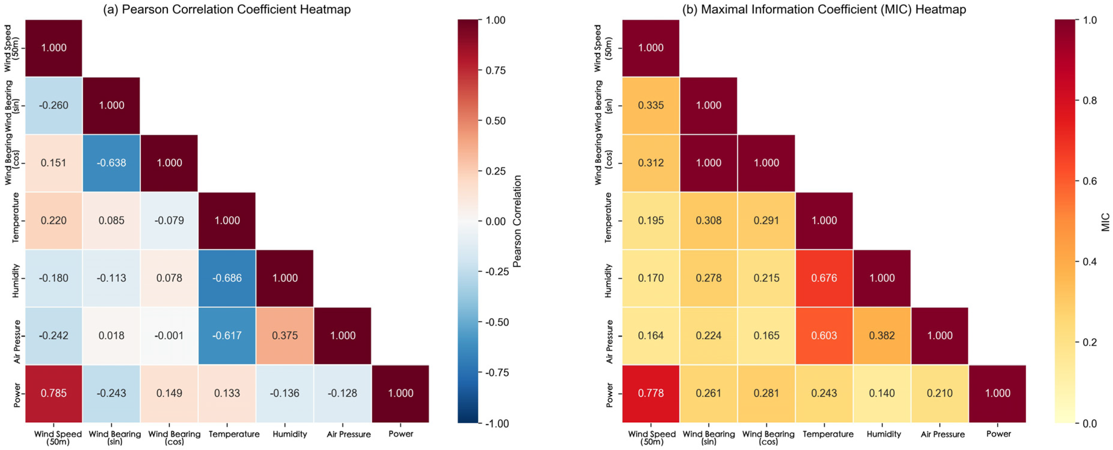
The 2019 wind power data of a wind power plant of Guohua Jingxia North Wind Power in Xinjiang Province were selected by using Pearson correlation analysis and MIC feature extraction methods, and the optimal feature input set was determined through comprehensive analysis from two angles. This dataset contains nine input characteristics of temperature, air pressure, wind speed, wind direction, and humidity at 10 m, 30 m, and 50 m; in order to achieve more accurate power prediction, this paper selects four of the nine input features from various angles to determine the final input feature set. Figure 1 and Figure 2 below include the Pearson correlation analysis heat map, the maximum mutual information coefficient heat map and the feature selection analysis.

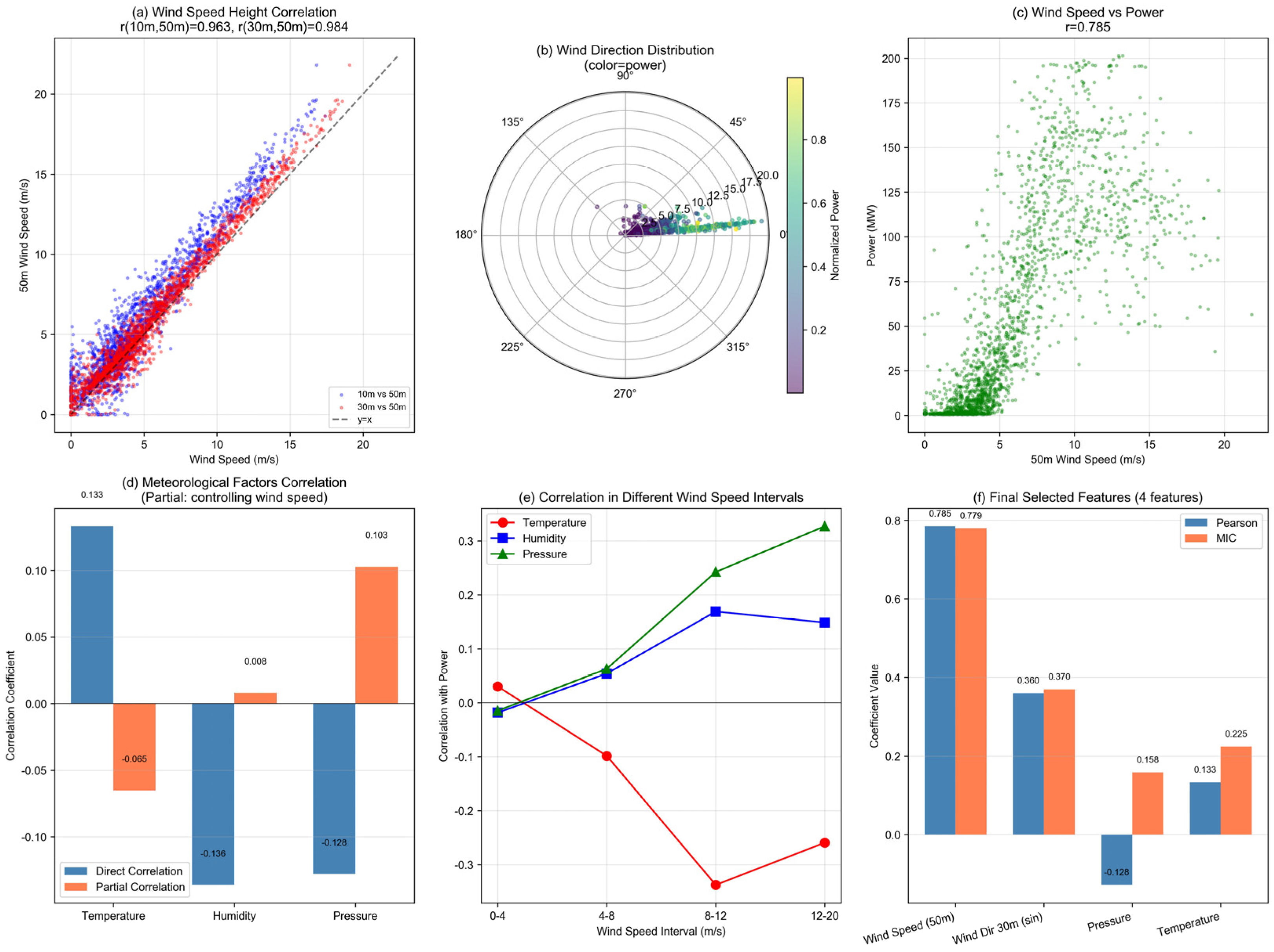
First of all, a 50 m wind speed is usually the best choice among the three wind speeds, because it is closer to the height of the wind turbine hub, is less affected by ground friction, and is more representative of free atmospheric flow. Through analysis, the correlation between 10 m and 50 m and between 30 m and 50 m in Figure 2a reaches 0.963 and 0.984, which shows that the correlation between wind speeds at different altitudes is strong and mutually replaceable, and the Pearson correlation coefficient and the maximum mutual information correlation coefficient of wind speed at 50 m reach 0.785 and 0.778, respectively, as shown in Figure 2; this is strongly correlated with power, so the wind speed at 50 m is selected as one of the final characteristic inputs, and Figure 2c is the power distribution map of different wind speeds at 50 m.

And in wind power prediction, wind direction is an important feature, because the power output of wind turbines is related to wind direction (yaw control, terrain influence, etc.). However, since the wind direction is angular and periodic, it cannot be directly used as a linear feature input, so the wind direction data is converted into a trigonometric function to calculate the correlation between wind direction data and power at different heights; Figure 2b is the distribution map of wind direction and power, and the two corresponding coefficients are shown in Figure 1. Finally, the wind direction at 30 m is determined as one of the final feature inputs.

Air density directly affects wind power and is positively correlated, while air density is determined by temperature, humidity and air pressure; when controlling the wind speed range, the direct correlation coefficients between temperature, humidity and air pressure are calculated as 0.133, −0.136 and −0.128, respectively, and the partial correlation coefficients are −0.065, 0.008 and 0.103, respectively. In Figure 2d, it can be found that the correlation between humidity and air pressure is consistent and the correlation of air pressure is stronger, and the correlation line diagram of temperature, humidity and air pressure and power in different wind speed intervals is calculated and drawn as shown in Figure 2e; it can be found that temperature and power are negatively correlated, humidity and air pressure are positively correlated with power, and the correlation between air pressure is stronger.

Therefore, temperature, the wind speed at 50 m, wind direction at 30 m and pressure were finally selected as the final feature inputs as shown in Figure 2f.

2.3. Improved Complete Ensemble Empirical Mode Decomposition with Adapted Noise

Marcelo et al. made further improvements on the basis of CEEMDAN, and proposed a decomposition algorithm called ICEEMDAN in 2014, which better solved the problems of residual noise and pseudomodality in CEEMDAN, and further improved the noise reduction effect and decomposition efficiency. If $f$ is set to be the signal to be decomposed and $M(\cdot )$ is the operator of the local mean, the ICEEMDAN calculation process is:

• Add $i$ sets of Gaussian white noise ${\xi }^i$ to the original sequence, and use EMD to calculate the local mean to construct sequence $f^i(t)=f(t)+{\epsilon }_0{E}_1({\xi }^i(t))$, and obtain the first set of residuals:

  $$r_1=〈M\left(f^i(t)\right)〉$$

  (3)

  where ${\epsilon }_0={\alpha }_0\sigma (x)/\sigma \left(E_1\left({\xi }^i\right)\right)$, $〈\cdot 〉$ represent the average.
• When $k=1$ is obtained, the first modal component is

  $$IM{F}_1(t)=f(t)-r_1(t)$$

  (4)
• $r_1$ is then processed from steps (1) to (2) to obtain the second residual $r_2$ and the second modal component:

  $$r_2=〈M\left(r_1(t)+{\epsilon }_1{E}_2\left({\xi }^i(t)\right)\right)〉$$

  (5)

  $$IM{F}_2(t)=r_1(t)-r_2(t)$$

  (6)
• Following the steps above, for $k=3,4,\dots ,K$, $r_k$ and $IM{F}_k(t)$ are calculated as

  $$r_k=〈M\left(r_{k-1}(t)+{\epsilon }_{k-1}{E}_k\left({\xi }^i(t)\right)\right)〉$$

  (7)

  $$IM{F}_k(t)=r_{k-1}(t)-r_k(t)$$

  (8)

2.4. Variational Mode Decomposition

VMD is a non-recursive signal processing algorithm that decomposes the original signal into several stable IMFs of different frequencies by iteratively solving the variational model. The expression is

$$\underset{{\mu }_k,{\omega }_k}{\min }=\left\{\sum _k{\partial }_t\left[\left(\delta (t)+{\displaystyle \frac{j}{\pi t}}\right)\ast e_k(t)\right]e^{-j\omega t2}\right\}$$

(9)

where $\ast$ is the convolutional operator; $e_k$ is the $k$-th subsequence. We can transform the constrained optimization problem in VMD into an unconstrained variational problem by introducing a Lagrangian multiplier $\lambda$ and a penalty factor $\alpha$. The expression is

$$\begin{array}{l}L\left(m_k,w_k,l\right)=\alpha {\displaystyle \sum _k}{\partial }_t\left[\left(\delta (t)+{\displaystyle \frac{j}{\pi t}}\right)\ast e_k(t)\right]{e^{-j{\omega }_{k^t}}}_2^2+f(t)-\\ {\displaystyle \sum _k}{e}_k{(t)}_2^2+〈\lambda (t),f(t)-{\displaystyle \sum _k}{e}_k(t)〉\end{array}$$

(10)

2.5. Sequence Frequency Partitioning Strategy Combined with Q Statistic and Sample Entropy

2.5.1. Q Statistic

In the context of signal decomposition, the Q statistic is usually defined as a measure of signal-to-noise ratio or relative reconstruction error. The basic idea is that if an IMF contains a large number of valid signals (e.g., periodic components, trends), its energy (or the contribution of its reconstructed signals) will be high relative to its own “fluctuations” (often considered noise), resulting in a higher Q value. Conversely, a pure-noise IMF will have a low Q value.

All IMFs are sorted or thresholds are set based on Q values. IMFs with high Q values are considered important and informative components that need to be retained; an IMF with a low Q value is considered a noise-dominant component and can be filtered out to achieve signal denoising. The corresponding formula for the Q statistic is

$$Q_i={\displaystyle \frac{E_{s,i}}{E_{n,i}}}={\displaystyle \frac{IM{F_i}_2^2}{Var\left(IM{F}_i\right)}}$$

(11)

$Q_i$: the quality index of the $i$-th eigenmodal function. $IM{F}_i$: the $i$-th eigenmodal function component. $E_{s,i}={‖IM{F}_i‖}_2^2$: The signal energy of the IMF. $E_{n,i}=Var\left(IM{F}_i\right)$: The variance of the IMF.

The larger the ratio, the more concentrated the energy and the more regular the oscillation, the higher the proportion of effective information it contains, and the better the quality. The Q statistic was used to classify the IMF, which was divided into three categories: primary signal, mixed component, and noise. Then two thresholds were set: threshold $T_1$ and threshold $T_2\left(T_1>T_2\right)$. This divides the IMF into three categories: high Q value $\left(Q_i\ge T_1\right)$—the main signal component (signal dominant); medium Q value $\left(T_1>Q_i\ge T_2\right)$—mixed components (signal and noise mixed); low Q $\left(Q_i<T_2\right)$—noise composition (noise dominant).

2.5.2. Sample Entropy

Sample entropy is a statistic that measures the complexity and irregularities of time series. Higher sample entropy reflects greater sequence complexity and irregularity; lower sample entropy implies enhanced regularity and predictability. For an IMF component, its sample entropy is calculated as

$$SampEn(z,r,N)=-\ln \left[{\displaystyle \frac{{\displaystyle \sum _{j=1}^{N-z}}{A}_j^{z+1}}{{\displaystyle \sum _{j=1}^{N-z}}{B}_j^z}}\right]$$

(12)

$z$: pattern length; $r$: similarity tolerance; $N$: time series length; $A_j^{m+1}$ and $B_j^m$ represent the number of vectors with the maximum value of the absolute value that satisfies the difference between the corresponding elements of the two vectors being less than or equal to $r$.

After calculating the sample entropy $E_i$, two thresholds $T_a$ and $T_b\left(T_a<T_b\right)$ are set; if $E_i\le T_a$, it is the effective signal component, the sample entropy is the lowest, and the sequence regularity is strong. If it is $T_a<E_i\le T_b$, it is a mixed component, and the sample entropy is medium, which is a mixture of signal and noise. If it is $E_i>T_b$, it is the noise component, the sample entropy is the highest, and the sequence is highly random and irregular.

2.5.3. Partitioning Strategy

The Q statistic evaluates IMF–signal correlation, generally indicating stronger correlation for low-frequency components and weaker correlation for high-frequency components. Sample entropy can measure the complexity of a sequence, with high-frequency components usually being more complex and with larger sample entropy values, while low-frequency components are more regular and have smaller sample entropy values. Therefore, the combination of the two can more accurately distinguish the components of different frequency bands, avoiding the boundary blurring problem that may be encountered when using only frequency features. Therefore, the specific division strategy used in this article is as follows:

• IMF component acquisition: The original signal is decomposed to obtain several IMFs.
• Feature extraction: The corresponding Q value and sample entropy value are calculated for each IMF component.
• Feature normalization processing: The Q value and sample entropy value are normalized to make their values between 0 and 1, eliminating the dimensional difference between features and making different features comparable. The specific calculation formula is

  $$Q_{norm-i}={\displaystyle \frac{Q_i-Q_{\min }}{Q_{\max }-Q_{\min }}}$$

  (13)

  $$E_{norm-i}={\displaystyle \frac{E_i-E_{\min }}{E_{\max }-E_{\min }}}$$

  (14)
• Weight determination and comprehensive scoring: For the Q value, the sample entropy and frequency are set as weights of ${\omega }_Q,{\omega }_E,{\omega }_F$, and the Q statistic is given a higher weight, because the Q value directly quantifies the representativeness or contribution of the component to the original signal and is the most intuitive measure of importance. Sample entropy and frequency are both indirect indicators (reflecting complexity and band position, respectively), and need to be combined with the Q value to have clear significance, and the sum of the weights of the three is 1, and the scoring formula is established as follows:

  $$Scor{e}_i={\omega }_Q\times Q_{norm-i}+{\omega }_E\times \left(1-E_{norm-i}\right)+{\omega }_F\times \left(1-F_{norm-i}\right)$$

  (15)

Here, $1-E_{norm-i}$ and $1-F_{norm-i}$ are inverted treatments, so that a high score corresponds to the low-frequency characteristics, and the higher the comprehensive score, the more the component is biased towards the low frequency.

5.

Classification decisions: The comprehensive score is ranked from high to low, the 30% and 70% quantiles of the comprehensive score are taken as thresholds, and finally, all IMFs are separated into three components with different frequencies.

2.6. Signal Secondary Decomposition Process

The IMF components obtained by ICEEMDAN are then divided into three frequency components by using the sequence frequency division strategy of combining Q statistics and sample entropy described above.

For the purpose of further reducing the influence of sequence randomness and complexity on the prediction model, VMD is used to carry out secondary refining of the high-frequency components obtained after the above ICEEMDAN decomposition, the above-mentioned sequence frequency division strategy is still used to obtain three frequency components after secondary refinement, and finally the high-frequency components obtained after the secondary decomposition are taken as the final high-frequency components, and the mid-frequency components obtained after the secondary decomposition are added to obtain the final mid-frequency components. The low-frequency component obtained after a decomposition is the final low-frequency component.

2.7. Evaluation Indicators

To accurately compare the prediction performance of each model, four error evaluation indicators are used in this paper.

$$RMSE=\sqrt{{\displaystyle \frac{1}{n}}{\displaystyle \sum _{i=1}^n(y_i-{y_i}^{\prime })}}$$

(16)

$$MAPE={\displaystyle \frac{1}{n}}{\displaystyle \sum _i^n\left|\frac{y_i-{y_i}^{\prime }}{y_i}\right|}\times 100\%$$

(17)

$$MAE={\displaystyle \frac{1}{n}}{\displaystyle \sum _i^n\left|y_i-{y_i}^{\prime }\right|}$$

(18)

$$R^2=1-{\displaystyle \frac{{\displaystyle \sum _i^n{(y_i-{y^{\prime }}_i)}^2}}{{\displaystyle \sum _i^n{(\overline{y}-{\overline{y}}^{\prime })}^2}}}$$

(19)

3. Combinatorial Prediction Model Construction Based on Improved Optimization Algorithm

3.1. Convolutional Neural Network

Convolutional neural networks (CNNs) are a kind of artificial neural network that leverage convolutional operations to automatically learn feature representations from data, and realize data identification and classification based on the extracted features.

A CNN captures local features in the input through the convolutional layer, reduces dimensionality and enhances features through the pooling layer, and then integrates the global information and outputs the final result through the fully connected layer. The network has the characteristics of local connection, weight sharing, and spatial hierarchical feature extraction, enabling it to efficiently handle complex tasks such as image recognition, behavior analysis, and natural language processing.

3.2. Bidirectional Gated Recurrent Neural Network

This network contains independent forward and reverse GRUs, which process past and future inputs respectively, and finally merge the outputs of the two. Therefore, better forecasting results can be obtained.

Considering that the splicing operation can completely retain the forward- and backward-timing-dependent features without introducing additional trainable parameters, it avoids the redundant parameters and gradient interference problems that may occur in the weighting or gating mode. The specific calculation process is

$$\left\{\begin{array}{l}{\overrightarrow{h}}_t=GRU\left(x_t,{\overrightarrow{h}}_{t-1}\right)\\ {\overleftarrow{h}}_t=GRU\left(x_t,{\overleftarrow{h}}_{t-1}\right)\\ h_t=\alpha {\overrightarrow{h}}_t+\beta {\overleftarrow{h}}_t+c_t\end{array}\right.$$

(20)

where ${\overrightarrow{h}}_t$ and ${\overleftarrow{h}}_t$ are the forward and backward hidden-layer outputs, respectively; $\alpha$ and $\beta$ represent the weights; and $c_t$ is the amount of hidden layer bias corresponding to $h_t$.

3.3. Global Attention Mechanism

The global attention mechanism is commonly used in sequence-to-sequence (Seq2Seq) models, and its core idea is to take into account all hidden states of the source sequence encoder while generating each word of the target sequence, and calculate a weight for each hidden state to determine its importance to the current decoding step.

When the time step is $t$, the specific calculation path is $h_t\to a_t\to c_t\to {\overline{h}}_t$, where $h_t$ and ${\overline{h}}_t$ represent the hidden state of the decoder side and the end point of the final output, respectively, $a_t$ represents the variable-length attention weight distribution vector, and $c_t$ is the context vector. The specific process is:

• Calculate the attention score. For the current state of the decoder $h_t$ and each encoder state ${\overline{h}}_s$, calculate a scalar score of $a_t$, which is used to measure the importance of ${\overline{h}}_s$ to $h_t$.
• Calculate the attention weight. All the scores obtained in the previous step are formed into a vector, the length is the time step $S$ at the encoder end, and the attention weight distribution $a_t$ is obtained by normalizing by the softmax function, and the calculation formula is

  $${\alpha }_t=soft\max (score(h_t,{\overline{h}}_s))={\displaystyle \frac{\exp (score(h_t,{\overline{h}}_s))}{{\displaystyle \sum _{s=1}^s}\exp (score(h_t,{\overline{h}}_s))}}$$

  (21)
• Calculate the context vector. The weighted average of all the weights $a_t$ obtained in (2) and the corresponding encoder state ${\overline{h}}_s$ is obtained to get the final context vector $c_t$:

  $$c_t=\sum _{s=1}^s{a}_t{\overline{h}}_s$$

  (22)
• Generate the final output. Finally, the implicit state $h_t$ of the decoder side and the context vector $c_t$ of the encoder side are combined to get the hidden state of the final attention layer, and the calculation formula is

  $${\overline{h}}_t=\tanh \left(\left[c_t;h_t\right]\right)$$

  (23)

3.4. Improved Gray Wolf Optimization Algorithm

3.4.1. Experience Exchange Strategy

The core concept of the EES stems from the learning and summary of group experience, and its goal is to improve the performance and effectiveness of meta-heuristic optimization algorithms. This strategy uses the historical position and current position of individuals in the population to convey empirical information, thereby strengthening the collaborative relationship between individuals and further enhancing the global search and local development capabilities.

As the search progresses, the population accumulates experience in the problem space. Based on this, the EES designs a variety of updated formulas to guide individuals to explore better solutions based on experience, thereby effectively improving the optimization ability of the algorithm. It specifically consists of three stages.

• Population and historical population:

  $$H_{p}os=Xpos=[po{s}_1,po{s}_2,\dots ,po{s}_N]$$

  (24)
• Empirical scarcity stage (ESC): In this stage, each individual has a large search range, so each search has a higher probability of obtaining a better fitness value. However, some algorithms still have difficulty achieving effective convergence in the empirical scarcity stage. For this problem, the EES focuses on the position information of individuals at this stage, and generates better fitness values by cross-manipulating the two candidate positions obtained through empirical exchange.

In the ESC stage, the algorithm selects two populations with certain search experience to generate new locations. Given that it remains in the initial phase of the search process, there are still a large number of unexplored areas in the solution space. Therefore, location updating mainly depends on the experience accumulated by a small number of populations, while the core driving force comes from the mechanism of individual exploration of new areas in the original algorithm.

$$EE{S}_{-}{H}_{-}pos\left(j\right)=\left\{\begin{array}{c}{H}_{-}pos\left(randi\left(N\right),j\right),rand<0.85\\ po{s}_{i,j},otherwise\end{array}\right.$$

(25)

$$po{s}_{-}EES\left(i,:\right)=pos\left(i,:\right)+\left(ES{C}_{-}{H}_{1-}pos-ES{C}_{-}{H}_{2-}pos\right)\times C$$

(26)

3.

Empirical crossover stage (ECR): With ongoing exploration of the search space, most algorithms gradually discover improved fitness values. Each individual accumulates rich exploration experience, and its position gradually evolves to a higher level of fitness. Finally, the new location is generated by updating the location through cross-operation based on different experienced individuals.

$$\begin{array}{l}po{s}_{EES}(i,:)=pos(i,:)+(EC{R}_{-}{H}_{1\_}pos-EC{R}_{-}{H}_{2\_}pos)\times r_1+\\ (EC{R}_{-}{H}_{1\_}pos-EC{R}_{-}{H}_{3\_}pos)\times (1-r)\times C\end{array}$$

(27)

4.

Experience sharing stage (ESH): At this stage, these individuals have accumulated rich experience, and the new location has a high reference value. At the end time, the group has focused on a better region, but at the same time, it is necessary to introduce a more refined local search mechanism to further improve the quality of the solution.

$$\begin{array}{l}po{s}_{-}EES(i,:)=(pos(i,:)+ES{H}_{-}{H}_{3-}pos)/2+\\ (ES{H}_{-}{H}_{1\_}pos-ES{H}_{-}{H}_{2\_}pos)\times r_2\times C\end{array}$$

(28)

5.

Select stage and historical position update: For the purpose of obtaining a better solution, the EES retains the optimal position through filtering and updates the historical position according to the following formula:

$$pos\left(i,:\right)=\left\{\begin{array}{c}po{s}_{-}EES\left(i,:\right),f\left(po{s}_{-}EES\left(i,:\right)\right)<f\left(pos\left(i,:\right)\right)\\ pos\left(i,:\right),\hspace{1em}otherwise\end{array}\right.$$

(29)

3.4.2. Specific Improvement Ideas

The “experience exchange strategy” was introduced in GWO. This strategy is usually executed after the standard location update step as an enhancement module. The specific steps are:

• Initialize: Initialize gray wolf population $X_i$. Initialization parameters: population size $N$, maximum number of iterations $T_{\max }$, coefficient vector $a,A,C$. Create an empty “experience library” of size $M$.
• Evaluate and rank: Calculate the fitness value of each gray wolf (i.e., the objective function value), and then sort the wolf pack to determine the current $X_{\alpha }(t),X_{\beta }(t),X_{\delta }(t)$.
• Standard GWO location update: Update the coefficient vector and the position of each $\omega$ wolf to get the new generation population $X_{new}$.
• Update the experience library: The experience library is used to store historically high-performing individuals or their variants, providing empirical reference for the population. Select elite individuals first: Select $top-K$ optimal individuals from the current new generation population. Then add the selected elite individuals to the experience pool $E$; if the experience pool is less than full (that is, the current size is less than $M$), then join directly; if the experience base is full, replace the least fitted individual in the experience base with a new elite individual.
• Exchange of experiences: Let some wolves learn from the pool of experience, not just from the current leadership. A random subset of individuals from the current population (usually $\omega$ wolf other than $\alpha ,\beta ,\delta$) is marked as $X_{learners}$. For each learner, one or more individuals are randomly selected from the experience database as their “experience mentors”, marked as $X_E$. Learners use weighted average learning to update their position based on the location information of the experienced tutor.
• Boundary processing and evaluation: Boundary checks are performed on the new positions generated after the experience exchange to prevent the solution from going beyond the search range, and the fitness value of this part of the experience exchange learner is recalculated.
• Elite retention: Compare the fitness values before and after the learner’s experience exchange, and if the post-swap position is worse, keep the pre-exchange position.
• Iterate through loops: Repeat steps 1 through 6 until the stopping criterion is met. After the algorithm is finished, the global optimal solution and its fitness value are output.

3.4.3. Optimization Algorithm Performance Test

To validate the performance and rationality of the improved GWO in this section, three aspects, including the classical single-peak function Sphere, the classical multimodal function Rastrigin, and $F_1,F_2,F_3,F_7,F_9,F_{10},F_{22},F_{29}$ in the CEC2017 test set, are selected to compare and validate the capability of the improved GWO algorithm. The parameter settings are as shown in

Table 1. Test function parameter settings.

Test Function	Dimension	Optimal	Value Range
Sphere	50	0	[−5.12, 5.12]
Rastrigin	50	0	[−5.12, 5.12]
$F_1$	50	100	[−100, 100]
$F_2$	50	200	[−100, 100]
$F_3$	50	300	[−100, 100]
$F_7$	50	700	[−1.28, 1.28]
$F_9$	50	900	[−5.12, 5.12]
$F_{10}$	50	1000	[−32, 32]
$F_{22}$	50	2200	[−100, 100]
$F_{29}$	50	2900	[−100, 100]

:

In order to further avoid chance and improve the persuasiveness of the superior performance of this improved algorithm, this paper uses the whale optimization algorithm WOA, the sparrow optimization algorithm SSA, the particle swarm optimization algorithm PSO, the improved sparrow optimization algorithm ISSA, the GWO and the EES-GWO in this paper for simulation experiments, and all algorithms are set with an overall scale of 50 and a maximum iteration count of 400 in the experiment.

3.4.4. Comparison of Different Algorithms

To minimize the influence of stochastic variability on the optimization results, 300 independent runs are conducted for each algorithm in this section, and we take the average, optimum, standard deviation and worst value of each algorithm for analysis. We prioritize the use of the average for ranking analysis and comparison, and compare the corresponding standard deviation if the mean is the same.

Table 2. Optimization results from different algorithms.

Function	Statistical Value	EES-GWO	GWO	WOA	PSO	SSA	ISSA
Sphere	Optimal	5.20 × 10−20	4.3 × 10−13	1.42 × 10−42	2.35 × 10−1	1.34 × 10−14	NaN
	Mean	3.15 × 10−38	1.02 × 10−12	9.65 × 10−37	5.44 × 100	2.26 × 10−12	3.33 × 10−38
	Standard Deviation	2.81 × 10−38	7.29 × 10−13	2.22 × 10−36	1.02 × 101	5.99 × 10−12	2.82 × 10−38
Rastrigin	Optimal	3.41 × 10−13	8.52 × 100	0	4.93 × 101	5 × 101	0
	Mean	7.43 × 100	1.69 × 101	0	7.02 × 101	6.97 × 101	0
	Standard Deviation	2.7 × 100	5.13 × 100	0	1.44 × 101	2.86 × 101	0
$F_1$	Optimal	1.46 × 10−33	1.63 × 10−7	1.83 × 10−35	8.1 × 103	5.46 × 10−13	NaN
	Mean	4.66 × 10−33	1.23 × 10−6	3.11 × 10−31	7.78 × 106	4.98 × 10−8	1.23 × 10−30
	Standard Deviation	2.24 × 10−33	9.75 × 10−7	5.11 × 10−31	2.16 × 107	7.95 × 10−8	3.67 × 10−30
$F_2$	Optimal	7.27 × 10−57	9.62 × 10−36	1.47 × 10−67	4.67 × 104	8.91 × 10−22	0
	Mean	1.27 × 10−51	6.76 × 10−29	2.63 × 10−51	1.01 × 1019	1.06 × 10−19	1.85 × 10−49
	Standard Deviation	2.3 × 10−48	1.87 × 10−28	7.8 × 10−51	3.03 × 1019	1.68 × 10−19	5.55 × 10−47
$F_3$	Optimal	2.67 × 101	7.91 × 102	2.88 × 104	1.01 × 104	2.05 × 103	NaN
	Mean	5.29 × 102	2.76 × 103	9.3 × 104	1.86 × 104	3.05 × 103	6.3 × 104
	Standard Deviation	4.65 × 102	2.01 × 103	2.4 × 104	5.9 × 103	5.05 × 102	2.52 × 104
$F_7$	Optimal	5.03 × 10−11	4.23 × 100	0	1.08 × 102	3.18 × 10−12	0
	Mean	9.15 × 100	3.4 × 101	5.68 × 101	1.85 × 102	6.69 × 101	0
	Standard Deviation	1.26 × 101	3.49 × 101	1.71 × 101	4.24 × 101	4.09 × 101	0
$F_9$	Optimal	9.04 × 10−1	7.25 × 10−1	1.12 × 10−1	5.47 × 10−1	3.6 × 10−1	1.99 × 100
	Mean	1.16 × 100	9.25 × 101	4.78 × 101	5.07 × 100	9.07 × 100	2.66 × 100
	Standard Deviation	2.2 × 10−1	1.65 × 101	4.22 × 10−1	4.14 × 101	7.43 × 100	3.27 × 10−1
$F_{10}$	Optimal	3.82 × 10−4	7.23 × 100	3.82 × 10−4	8.69 × 102	5.66 × 103	3.82 × 10−4
	Mean	3.82 × 10−4	1.5 × 102	7.58 × 10−2	1.58 × 103	6.61 × 103	1.5 × 101
	Standard Deviation	1.65 × 101	1.7 × 102	2.26 × 10−1	6.04 × 102	7 × 102	7.2 × 10−10
$F_{22}$	Optimal	2.56 × 10−10	2.16 × 100	0	5.47 × 101	6.43 × 10−12	2.05 × 100
	Mean	2.43 × 100	1.26 × 101	2.84 × 101	9.3 × 101	2.98 × 101	5.03 × 100
	Standard Deviation	2.74 × 100	6.42 × 100	8.53 × 101	2.12 × 101	1.72 × 101	4.12 × 100
$F_{29}$	Optimal	1.61 × 101	1.61 × 101	1.46 × 100	9.23 × 101	1.72 × 101	1.73 × 101
	Mean	1.65 × 101	1.68 × 101	8.58 × 100	9.32 × 102	1.72 × 101	1.74 × 101
	Standard Deviation	3.35 × 10−3	3.92 × 10−1	7.13 × 100	8.64 × 102	8.71 × 10−3	6.93 × 10−3

below presents the optimization results of each algorithm.

Table 2 shows that among these test functions, EES-GWO has the highest test accuracy and the best comprehensive performance in the test functions Sphere and $F_1,F_2,F_3,F_9,F_{10},F_{29}$, but its Rastrigin’s test accuracy is slightly less than that of WOA and ISSA, its $F_7$ test accuracy is slightly less than that of ISSA, and its $F_{22}$ test accuracy is slightly less than that of WOA. Moreover, EES-GWO has the smallest standard deviation of the test functions Sphere and $F_1,F_2,F_3,F_9,F_{22},F_{29}$, the algorithm operation results are more concentrated and stable, the standard deviation performance on Rastrigin and $F_{10}$ is slightly inferior to WOA and ISSA, and the standard deviation on $F_7$ is second only to ISSA. In summary, the EES-GWO has the best optimization ability on the model.

3.4.5. Homologous Comparison

For the purpose of further validating the optimization ability of the improved optimization algorithm, this section proposes a homologous improved optimization comparison, and three improved optimization strategies are selected to compare and verify their respective effects on the optimization performance of GWO, and the same experimental environment is adopted.

The selected improved optimization algorithms are EGWO (adding a module for parallel calculation and selecting reverse solutions in the algorithm flow), RGWO (modifying the position update formula and optimizing from the level of search behavior), IGWO (using a random exchange strategy), GWO, and the EES-GWO proposed in this paper. We prioritize the use of the average for ranking analysis and comparison, and compare the corresponding standard deviation if the mean is the same.

Table 3. Homologous improvement optimization results.

Function	Statistical Value	GWO	EGWO	IGWO	RGWO	EES-GWO
Sphere	Optimal	2.30 × 10−13	1.26 × 10−16	1.92 × 10−6	8.89 × 10−14	5.20 × 10−20
	Mean	1.56 × 10−12	4.27 × 10−15	7.39 × 10−6	1.54 × 10−12	2.63 × 10−18
	Standard Deviation	1.46 × 10−12	4.70 × 10−15	5.21 × 10−6	1.49 × 10−12	4.84 × 10−18
Rastrigin	Optimal	5.84 × 100	7.43 × 10−11	9.57 × 100	4.06 × 100	1.14 × 10−13
	Mean	1.98 × 101	9.83 × 100	3.33 × 101	1.95 × 101	1.51 × 101
	Standard Deviation	8.72 × 100	1.36 × 101	2.09 × 101	1.27 × 101	3.31 × 101
$F_1$	Optimal	1.24 × 10−7	1.73 × 10−10	1.25 × 100	9.54 × 10−8	4.29 × 10−14
	Mean	1.22 × 10−6	2.70 × 10−9	5.34 × 100	9.74 × 10−7	1.50 × 10−12
	Standard Deviation	1.14 × 10−6	3.71 × 10−9	4.05 × 100	1.53 × 10−6	2.28 × 10−12
$F_2$	Optimal	1.46 × 10−36	7.00 × 10−48	1.82 × 10−15	4.48 × 10−37	1.33 × 10−58
	Mean	2.37 × 10−29	1.09 × 10−37	2.09 × 10−7	7.35 × 10−28	4.16 × 10−44
	Standard Deviation	1.13 × 10−28	5.56 × 10−37	1.08 × 10−6	3.95 × 10−27	2.10 × 10−43
$F_3$	Optimal	1.52 × 102	2.38 × 101	7.22 × 102	1.26 × 102	7.81 × 100
	Mean	2.30 × 103	9.09 × 102	4.42 × 103	2.00 × 103	7.23 × 102
	Standard Deviation	2.42 × 103	9.99 × 102	2.32 × 103	1.48 × 103	1.53 × 103
$F_7$	Optimal	4.23 × 100	2.24 × 100	2.39 × 101	1.23 × 101	1.03 × 10−11
	Mean	2.65 × 101	1.47 × 101	4.20 × 101	3.22 × 101	6.30 × 100
	Standard Deviation	2.24 × 101	1.00 × 101	9.49 × 100	4.37 × 101	8.73 × 100
$F_9$	Optimal	5.42 × 10−1	6.61 × 10−1	5.45 × 10−1	6.42 × 10−1	6.42 × 10−1
	Mean	1.00 × 100	1.09 × 100	1.06 × 100	1.04 × 100	1.13 × 100
	Standard Deviation	2.10 × 10−1	2.28 × 10−1	2.97 × 10−1	2.28 × 10−1	2.61 × 10−1
$F_{10}$	Optimal	7.19 × 100	3.82 × 10−4	1.01 × 101	2.98 × 10−1	3.82 × 10−4
	Mean	1.77 × 102	4.92 × 101	6.36 × 102	2.08 × 102	1.10 × 101
	Standard Deviation	2.78 × 102	8.62 × 101	5.21 × 102	2.42 × 102	1.53 × 101

below shows the simulation results.

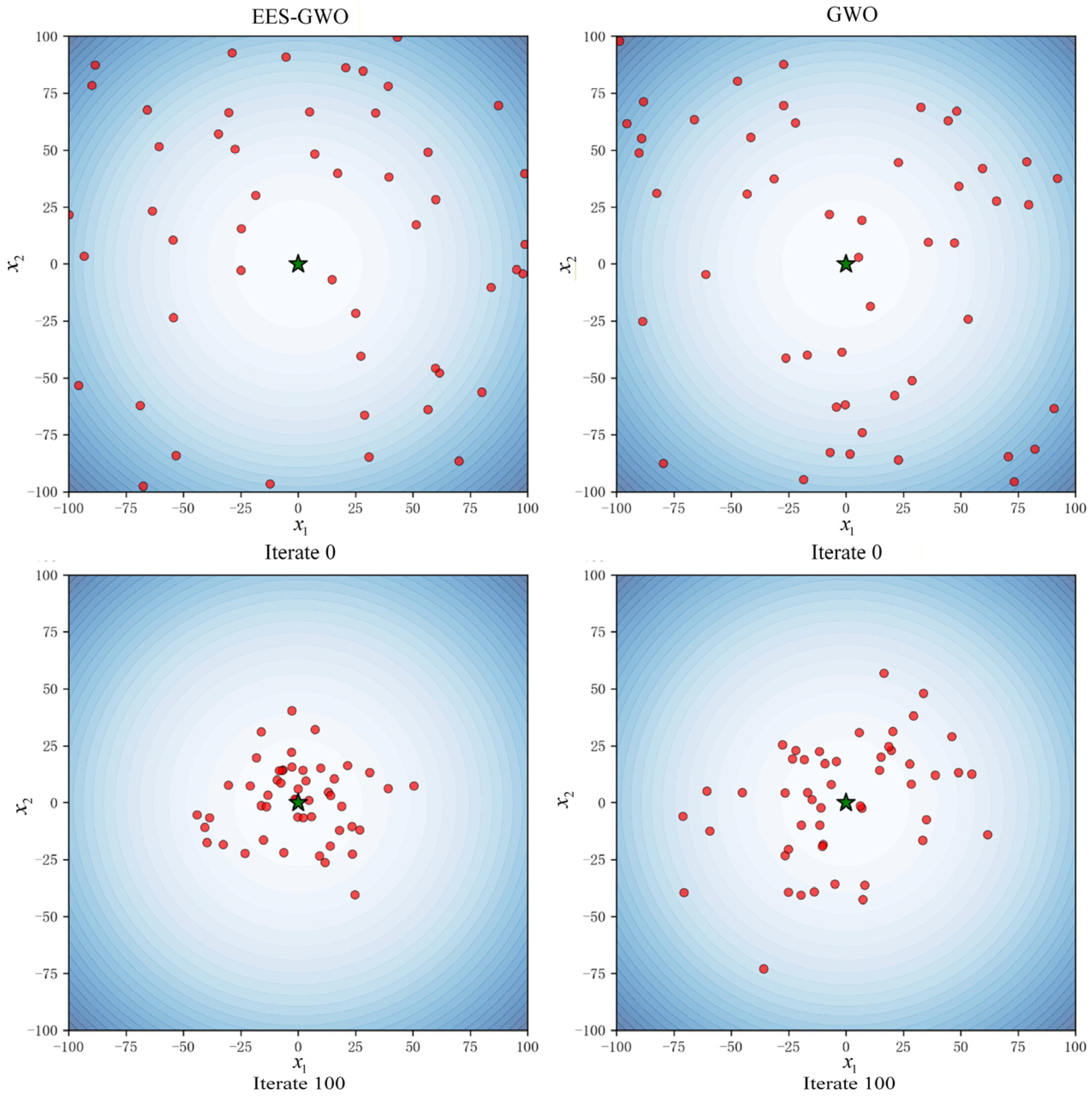
Table 3 shows that in the test functions Sphere and $F_1,F_2,F_3,F_7,F_{10}$, the optimization performance of EES-GWO mentioned in this paper is the best compared with others; specifically, in the function Sphere and $F_1,F_2,F_3,F_7,F_{10}$, the optimization performance of EGWO and RGWO is slightly inferior to EES-GWO, but it is significantly improved compared with GWO. In the function Rastrigin, EGWO has the best optimization performance, followed by EES-GWO, which is better than other improved methods. In function $F_9$, the optimization ability of all optimization algorithms is very similar, but the performance is slightly worse than that of GWO. The population distribution map of EES-GWO and GWO with 0 and 100 iterations is shown in Figure 3, which shows that the population convergence ability of EES-GWO is significantly improved compared with GWO.

3.4.6. High-Frequency Model Optimization Process

In this paper, the CNN-BiGRU–Global attention high-frequency component prediction model is constructed, and then the GWO algorithm improved by the EES is introduced, which is essentially a meta-heuristic hyperparameter optimization method. The core idea is to transform the hyperparameter optimization problem of deep learning into a search problem in a continuous space, and find the optimal combination of hyperparameters through bionic intelligent algorithms.

The core logic of the whole process is to encode the various discrete and continuous hyperparameters of the CNN-BiGRU–Global attention model into a continuous position vector. The EES-GWO algorithm is used to search for the optimal solution in this high-dimensional parameter space. The model performance corresponding to the hyperparameter is used as the fitness value of the search algorithm to guide the search direction. Finally, through multiple iterations, the optimal hyperparameter configuration is gradually approached.

The specific optimization steps are as follows:

Step 1: First, clarify the hyperparameter range of the CNN-BiGRU–Global attention model to be optimized. These parameters include:

CNN component parameters: Number of convolutional layers, number of convolutional cores. BiGRU component parameters: Number of loop layers, dropout rate. Global attention parameters: Attention dimension, attention heads. Training parameters: Learning rate.

These parameters are uniformly encoded to form a multi-dimensional position vector. The value of each dimension corresponds to a specific hyperparameter, and the continuous algorithm space values are converted into actual hyperparameter values through discrete mapping rules.

Step 2: Algorithm initialization and population establishment.

The parameters of the EES-GWO algorithm are initialized, including the number of gray wolf populations, the maximum number of iterations, and the size of the experience library. Each gray wolf in the initial population represents a random set of hyperparameter combinations. At the same time, an empty empirical database is established to store the excellent solutions found during the search process.

Step 3: Iteratively optimize the main loop.

The optimization process is carried out in the following steps until the maximum number of iterations is reached or the convergence conditions are met:

(1)

Fitness assessment stage: For each gray wolf in the population (each set of hyperparameters), the position vector of each gray wolf is first decoded, and the specific hyperparameter configuration is obtained, and then the CNN-BiGRU–Global attention model is constructed according to these configurations. The training data is then used to train the model in a limited number of rounds, evaluate the model performance on the validation set, take this performance as the fitness value of the gray wolf, and finally record the optimal position of the individual and the global optimal position.

(2)

Leadership determination stage: The gray wolf population was ranked according to fitness values, and the three wolves with the highest fitness were identified as $\alpha$ wolves, $\beta$ wolves, and $\delta$ wolves, which represent the currently found combination of the best, second-best, and third-best hyperparameters.

(3)

Standard position update stage: In addition to the leading wolf, other gray wolves ($\omega$ wolves) update their positions according to the mathematical formulas of the standard gray wolf optimization algorithm. This process simulates the behavior of wolves following the leader hunting, and tends to gather towards the current optimal solution area, reflecting the development ability of the algorithm.

(4)

Experience base update stage: Save the positions (hyperparameter combinations) of the top performing wolves (usually $\alpha ,\beta ,\delta$ wolves) in the current iteration to the experience library. If the experience pool is full, update the experience in the library by replacing the worst solution according to the established strategy.

(5)

Experience exchange stage: A part of the gray wolf is randomly selected as the learner, the experience is randomly selected from the experience database as the tutor, and the weighted learning method is used to comprehensively consider the learner’s current position, the tutor’s experience, and the global optimal solution for experience exchange.

(6)

Boundary treatment and elite retention: Make sure that the updated position is still within the preset hyperparameter value. For values that are outside the boundary, truncate or map them. And adopt the greedy selection strategy, and accept the new position only after the experience exchange is improved to ensure convergence.

Step 4: Result output and final verification.

3.5. Prediction Model of Low- and Mid-Frequency Components Based on XGBoost

According to its characteristics, the EES-GWO-CNN-BiGRU–Global attention high-frequency component prediction model is constructed in Section 3, and the medium-frequency and low-frequency components decomposed in Section 2 usually represent the trend and periodic components of wind power, which are affected by weather systems, day and night changes, etc., and the laws are relatively obvious and easy to model. Therefore, focusing on the low-frequency components can reduce noise interference and make the model more stable and accurate. XGBoost can effectively handle nonlinear relationships and feature interactions, and has strong overfitting resistance, making it suitable for learning complex mapping between low- and mid-frequency components and meteorological factors and historical power.

The XGBoost model is a powerful boosting library that integrates linear-scale solvers and tree-based machine learning algorithms. Compared with the traditional GBDT algorithm, XGBoost is more innovative in the handling of loss functions, using second-order Taylor expansions, combining first-order and second-order derivatives, and introducing regular terms. This allows XGBoost to comprehensively consider the downward trend of the objective function and the complexity of the model, so as to effectively prevent overfitting in the process of optimizing the overall solution.

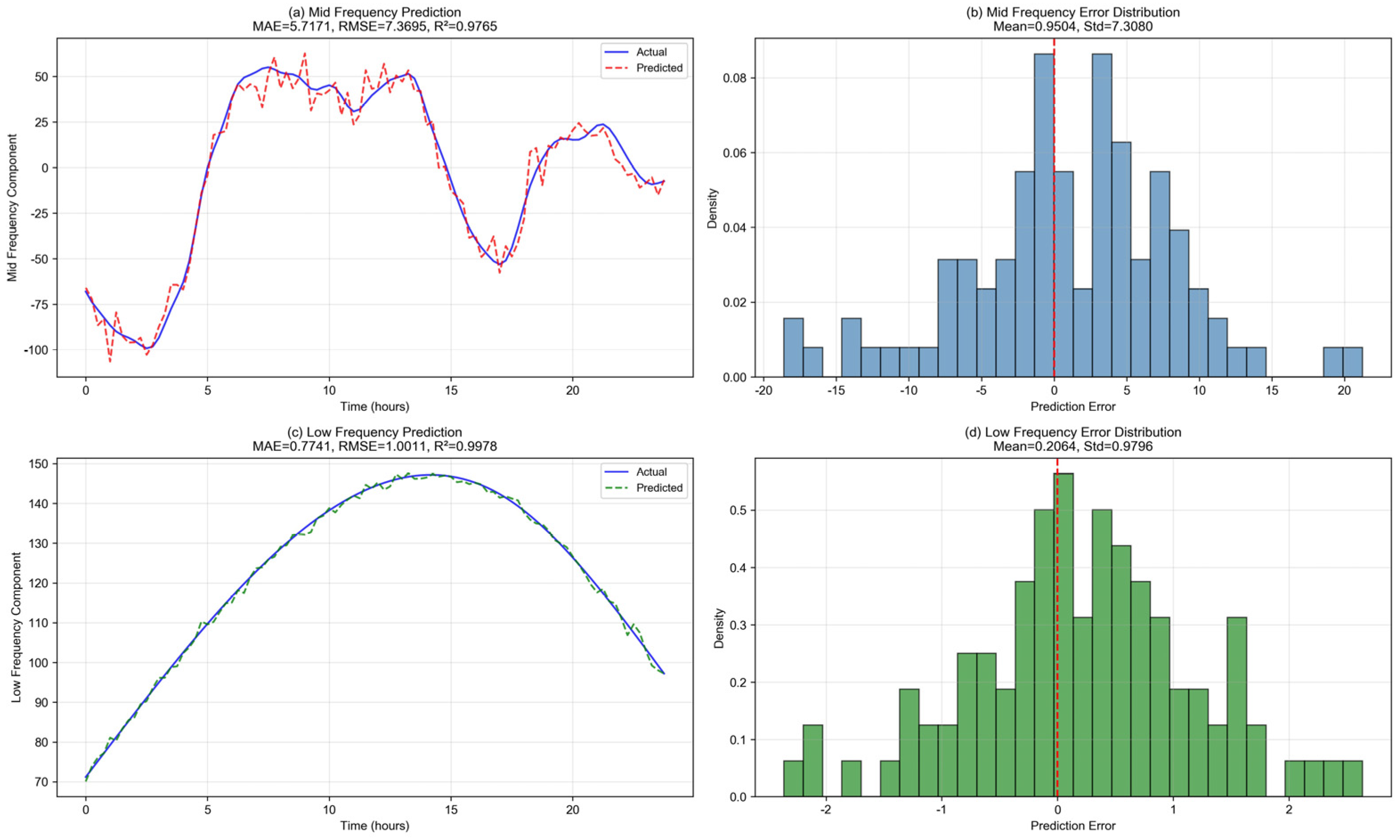
In light of the above, this work proposes an XGBoost-based prediction model for the mid- and low-frequency components obtained from Section 2. Using data from 1 to 20 March as the training set and 21 March as the test set, the model takes these components as inputs. To present the prediction results more intuitively, Figure 4 illustrates the prediction curve and error distribution for the mid- and low-frequency components using the 21 March input data.

It is evident from Figure 4 that the XGBoost-based prediction model for medium- and low-frequency components effectively captures the original power data, indicating favorable prediction performance, and the prediction error of the corresponding mid- and low-frequency components in March is concentrated; the prediction accuracy performs well.

3.6. Research on Multi-Model Fusion Wind Power Prediction Based on Improved Optimization Algorithm

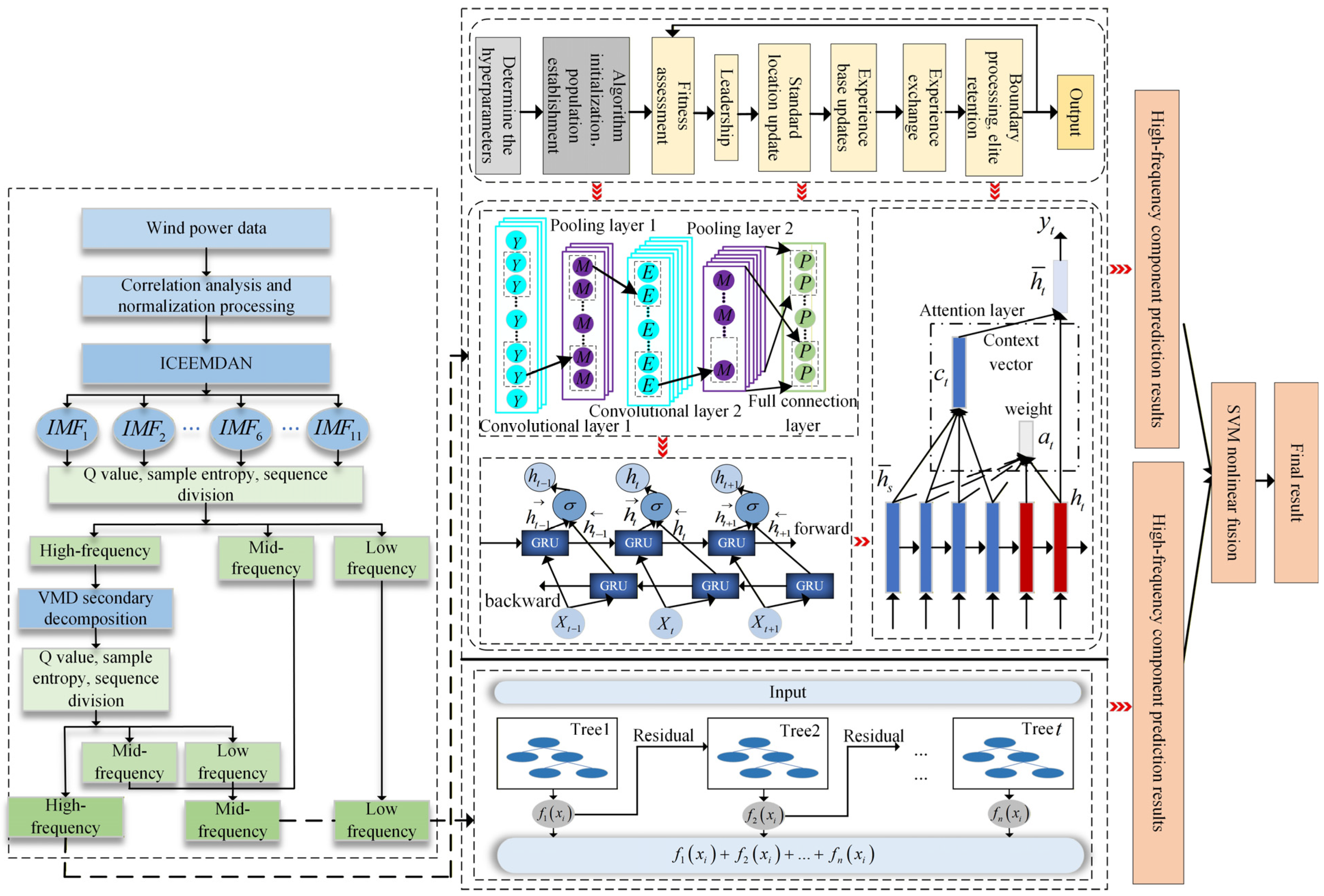
For the purpose of achieving more accurate wind power prediction, the ICEEMDAN-VMD-EES-GWO-CBG-XGBoost-SVM fusion model is proposed. As a first step, correlation analysis is carried out on the original dataset and after determining the final input feature set, the data is decomposed using ICEEMDAN to obtain several IMF components, and the sequence frequency division strategy combining Q statistic and sample entropy value is used to divide it into three different frequency components. This high-frequency component is the final high-frequency component, and the mid- and the low-frequency components obtained by secondary decomposition are added to obtain the final mid-frequency component, and the low-frequency component gotten by the first decomposition is the final low-frequency component.

Then, the experience exchange strategy, EES, is introduced into GWO, and the optimization performance of EES-GWO proposed in this paper is verified from two perspectives: optimization comparison of different optimization algorithms and homology improvement optimization comparison. Then, the EES-GWO-CBG model is constructed to forecast the high-frequency components, and the XGBoost model is constructed to forecast the mid- and low-frequency components. Finally, considering that the direct superposition of component forecasting results will affect the results, in this paper, the prediction results of all frequency components are fed into the SVM model and mapped to the high-dimensional space through a nonlinear transformation to achieve nonlinear fusion, and the ultimate prediction results are obtained. Simply adding the prediction results of each component ignores the isolinear assumption, prediction accuracy difference and nonlinear interaction. SVM fusion can adaptively learn the nonlinear combination weights of each component, suppress the influence of outliers, and correct systematic bias, so as to obtain better prediction accuracy and robustness. Figure 5 shows the model structure of this paper.

4. Example Analysis

4.1. Signal Decomposition

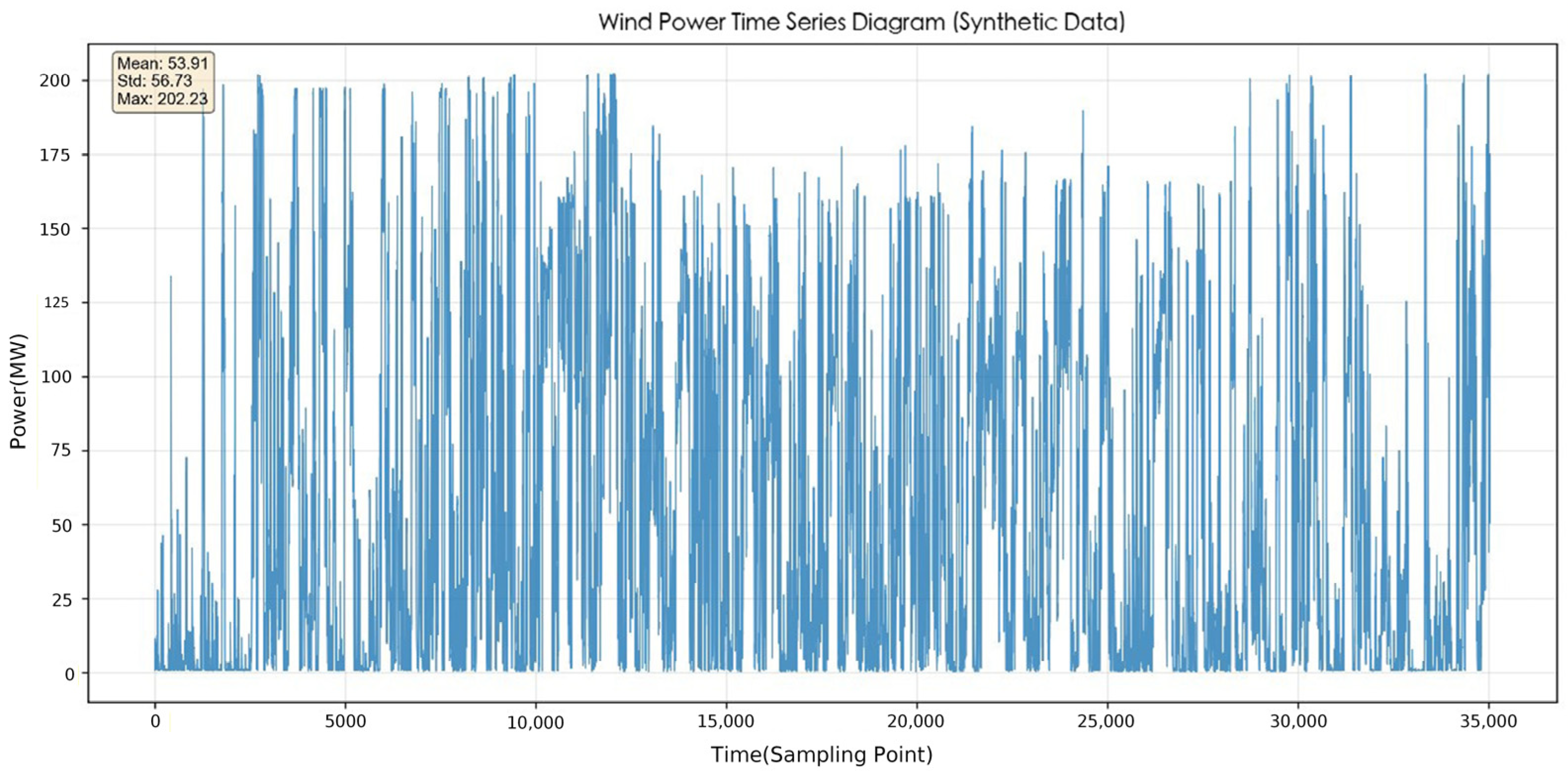
In this section, input data are obtained from the 2019 wind power project of Xinjiang Guohua Jingxia North Wind Power Plant, with a sampling interval of 15 min and a total of 35,040 sets of data, and the original wind power sequence curve is shown in Figure 6.

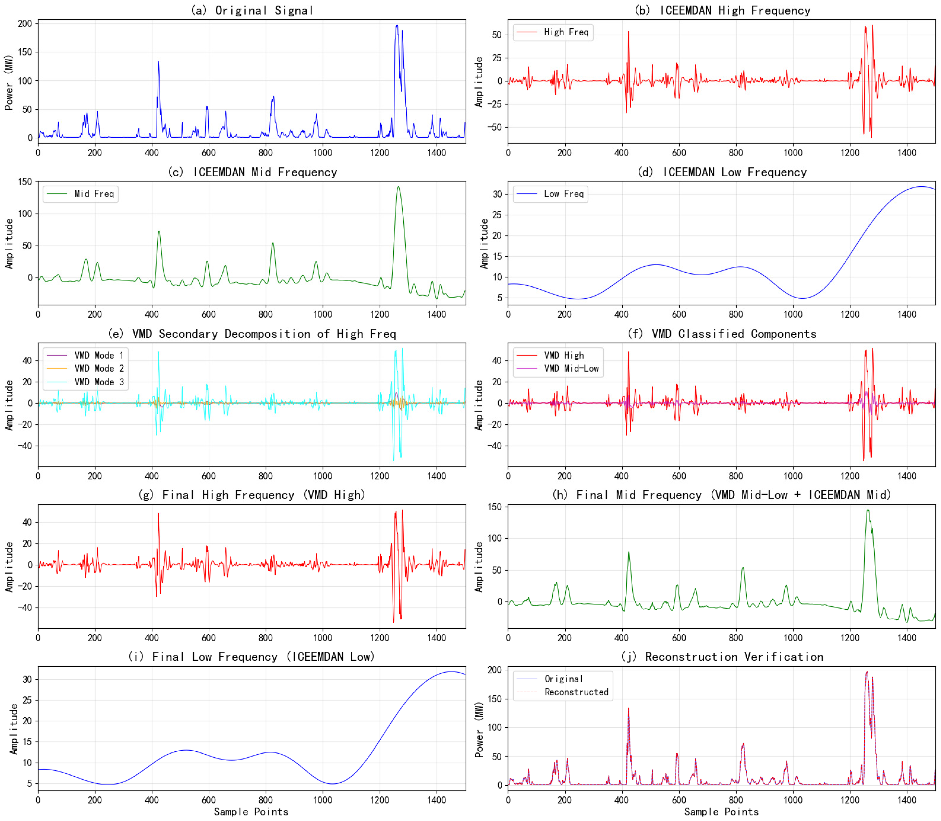
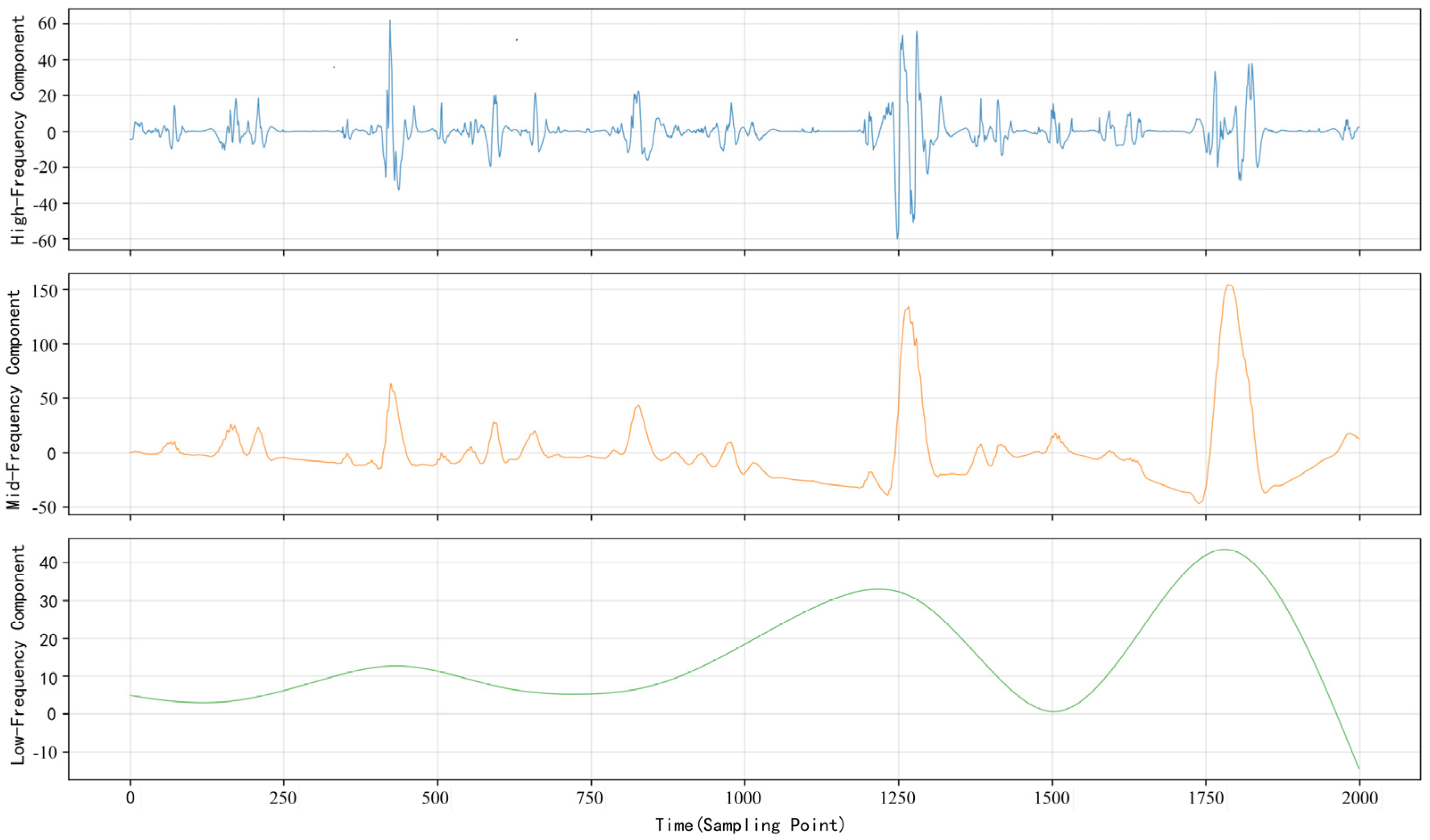
The Q value and sample entropy value of each IMF are calculated, the frequency of the two and each sequence itself is combined, and the corresponding weights are set to establish a comprehensive scoring function. The comprehensive scoring threshold is set to the high-frequency threshold of 0.37 and the low-frequency threshold is −14.01. The calculation results of the Q value and sample entropy value are shown in

Table 4. Q values and sample entropy calculation results.

$\mathit{I}\mathit{M}\mathit{F}$	Q Value	Sample Entropy	Average Frequency	Composite Score	Frequency Classification
$IM{F}_1$	1227.393	0.153799	0.111182	11.42884	High Frequency
$IM{F}_2$	4728.879	0.143426	0.036693	0.374635	High Frequency
$IM{F}_3$	10,660.09	0.151755	0.014648	−7.67772	Medium Frequency
$IM{F}_4$	13,684.16	0.128631	0.007617	−11.6362	Medium Frequency
$IM{F}_5$	14,817.19	0.051725	0.002881	−14.0119	Low Frequency
$IM{F}_6$	14,594.6	0.021926	0.002839	−14.0915	Low Frequency
$IM{F}_7$	14,764.4	2.60 × 10−05	0.002887	−14.4754	Low Frequency

; the decomposition process and the final result of decomposition are shown in Figure 7 and Figure 8.

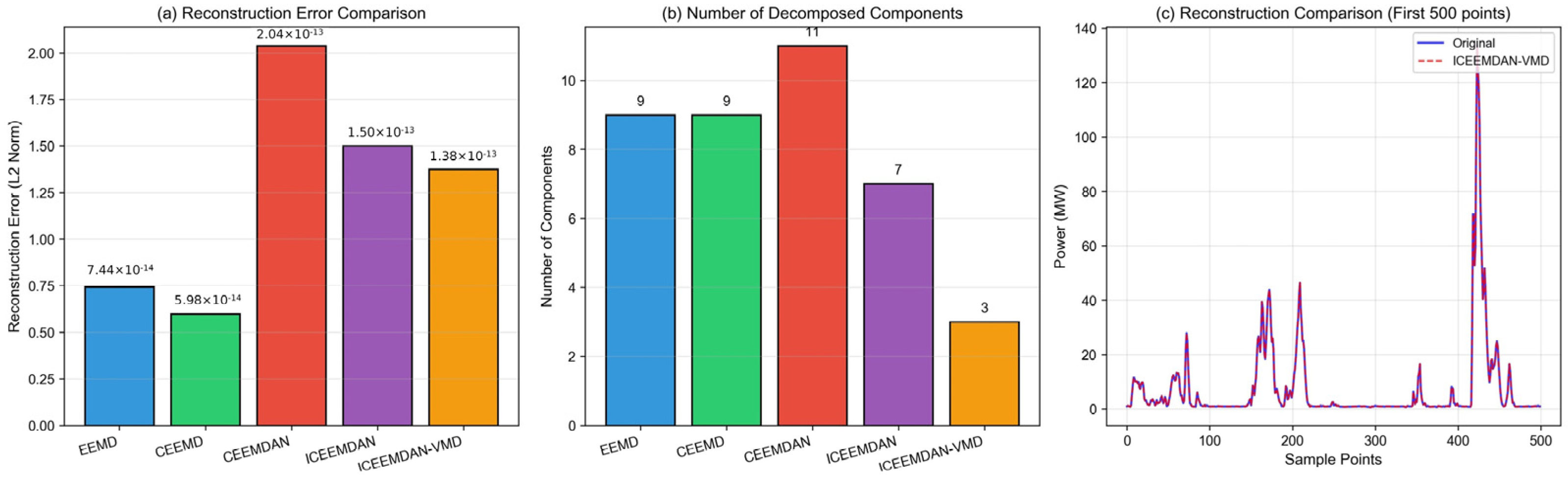
Aiming at validating the superiority of the secondary decomposition of the proposed decomposition algorithm ICEEMDAN-VMD, EEMD, CEEMD, CEEMDAN and ICEEMDAN are used for comparative simulation analysis, and several new sets of power sequences are obtained by adding and reconstructing the sequence components obtained after decomposition by the above decomposition algorithms, and then the new power sequence is differentiated from the original power sequence, and the reconstruction error of each decomposition algorithm is obtained as shown in Figure 9.

As can be seen from Figure 8, the ICEEMDAN-VMD quadratic decomposition method achieves significant improvements over other decomposition algorithms, exhibiting the smallest reconstruction error and the closest fit to the original time series.

4.2. Comparison of High-Frequency Component Prediction Models Under Different Optimization Algorithms

This example analysis selects the wind power data of a wind power plant in March and September 2019 of GuoHua Jingxia North Wind Power in Xinjiang Province, in which data from 1 to 20 days are selected as the training set for each month of March and September, with a total of 1920 sets of data. The data on the 21st was selected as the test set, with a total of 96 sets of data.

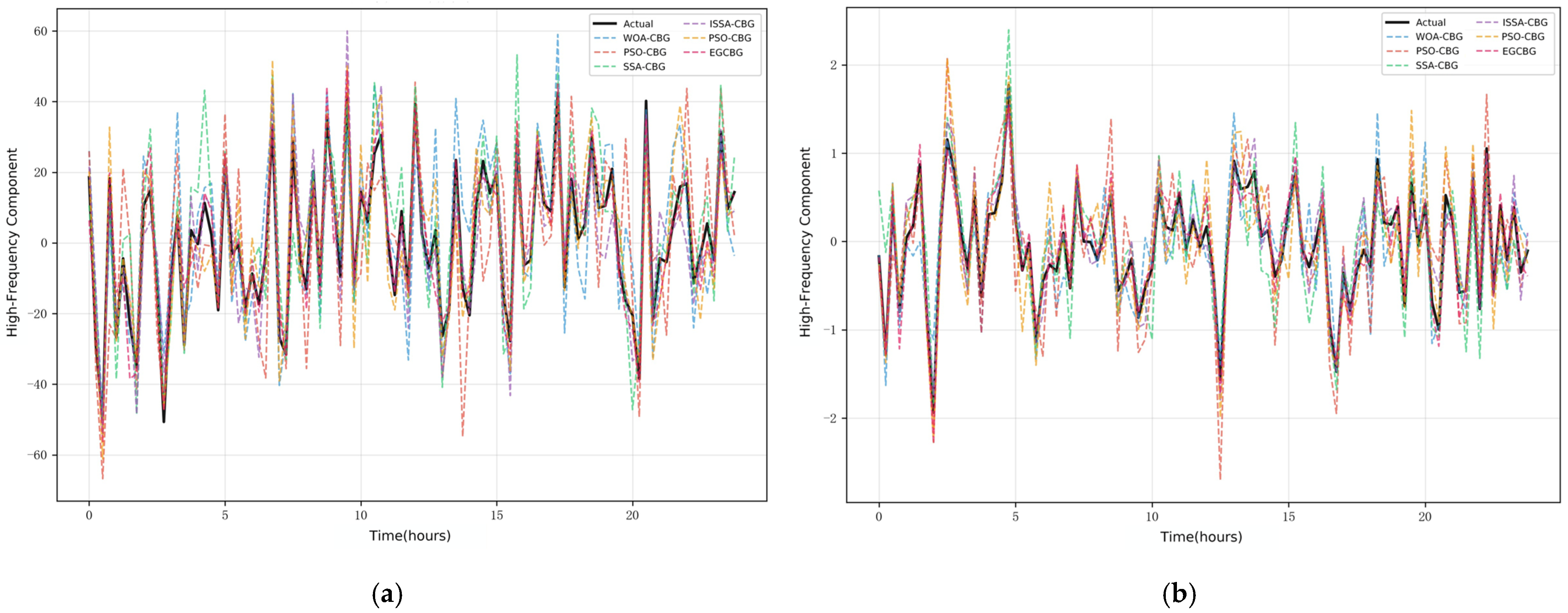
To verify the optimization performance of the EES-GWO algorithm, the WOA-CBG model, the PSO-CBG model, the SSA-CBG model, the ISSA-CBG model, and the GWO-CBG model are simulated and compared with the EES-GWO-CBG model, and the parameter setting is the same as above. The evaluation indicators of each model in March and September are calculated as shown in

Table 5. Evaluation index of high-frequency component prediction model.

Time	Predictive Models	Evaluation Indicators
		MAE (MW)	RMSE (MW)	MAPE (MW)	${\mathit{R}}^2$
March	WOA-CBG	0.496116	0.643625	50.66589	0.99694
	PSO-CBG	0.624234	0.764685	41.69329	0.995681
	SSA-CBG	0.541777	0.666437	71.80914	0.996719
	ISSA-CBG	0.401654	0.515404	24.13652	0.998038
	GWO-CBG	0.49319	0.615672	25.43896	0.9972
	EES-GWO-CBG	0.279026	0.342446	19.74676	0.999134
September	WOA-CBG	0.028672	0.037197	34.85722	0.99694
	PSO-CBG	0.036076	0.044193	32.94344	0.995681
	SSA-CBG	0.029469	0.038813	26.84957	0.996669
	ISSA-CBG	0.017934	0.023247	16.98061	0.998805
	GWO-CBG	0.028503	0.035581	26.07123	0.9972
	EES-GWO-CBG	0.016126	0.019791	14.32122	0.999134

.

It can be seen from Table 5 that in March and September, the forecasting accuracy of the EES-GWO-CBG model is significantly improved compared with the models under other optimization algorithms.

For example, in September, the MAPE, MAE and RMSE of the EES-GWO-CBG prediction model are the smallest and the $R^2$ is closer to 1, indicating that the curve fit is better.

For the purpose of intuitively comparing the fitting degree across models, the prediction curve of each model using the data of March and 21 September as input is plotted, as shown in Figure 10. It can be seen that the EES-GWO-CBG model is closest to the actual power in March and September.

4.3. Comparison of Prediction Model Results Under Different Decomposition Algorithms

To verify the performance of the ICEEMDAN-VMD quadratic decomposition algorithm proposed herein when applied to the prediction model, EEMD, CEEMD, CEEMDAN, ICEEMDAN and the proposed model are used for simulation comparison, and the final results of the evaluation indicators for June and December are shown in

Table 6. Evaluation metrics of different decomposition algorithms for prediction models.

Time	Predictive Models	Evaluation Indicators
		MAE (MW)	RMSE (MW)	MAPE (MW)	${\mathit{R}}^2$
June	EEMD	2.04966	2.447883	224.9493	0.944765
	CEEMD	2.300075	2.56563	232.1736	0.939323
	CEEMDAN	1.888448	2.171625	203.2252	0.956529
	ICEEMDAN	1.873764	2.123551	200.2925	0.958432
	ICEEMDAN-VMD	0.399196	0.501488	40.98006	0.997682
December	EEMD	0.982883	1.211468	82.65501	0.982055
	CEEMD	2.300331	3.066079	99.41811	0.885058
	CEEMDAN	0.843851	1.009503	72.89789	0.98754
	ICEEMDAN	0.81952	0.965544	71.4807	0.988601
	ICEEMDAN-VMD	0.237579	0.317859	19.91208	0.998765

.

As shown in Table 6, the ICEEMDAN-VMD quadratic decomposition algorithm outperforms other prediction models in terms of accuracy, demonstrating a substantial enhancement across the months examined.

For example, for the June indicators, the MAPE, MAE and RMSE of the ICEEMDAN-VMD prediction model are the smallest and the $R^2$ is closer to 1, indicating that its curve fit is better and the prediction accuracy is higher. In December, the ICEEMDAN-VMD quadratic decomposition algorithm still has great advantages compared with other decomposition algorithms; the MAPE, MAE, and RMSE are still much lower than those of other decomposition algorithms; and the fitting degree is excellent.

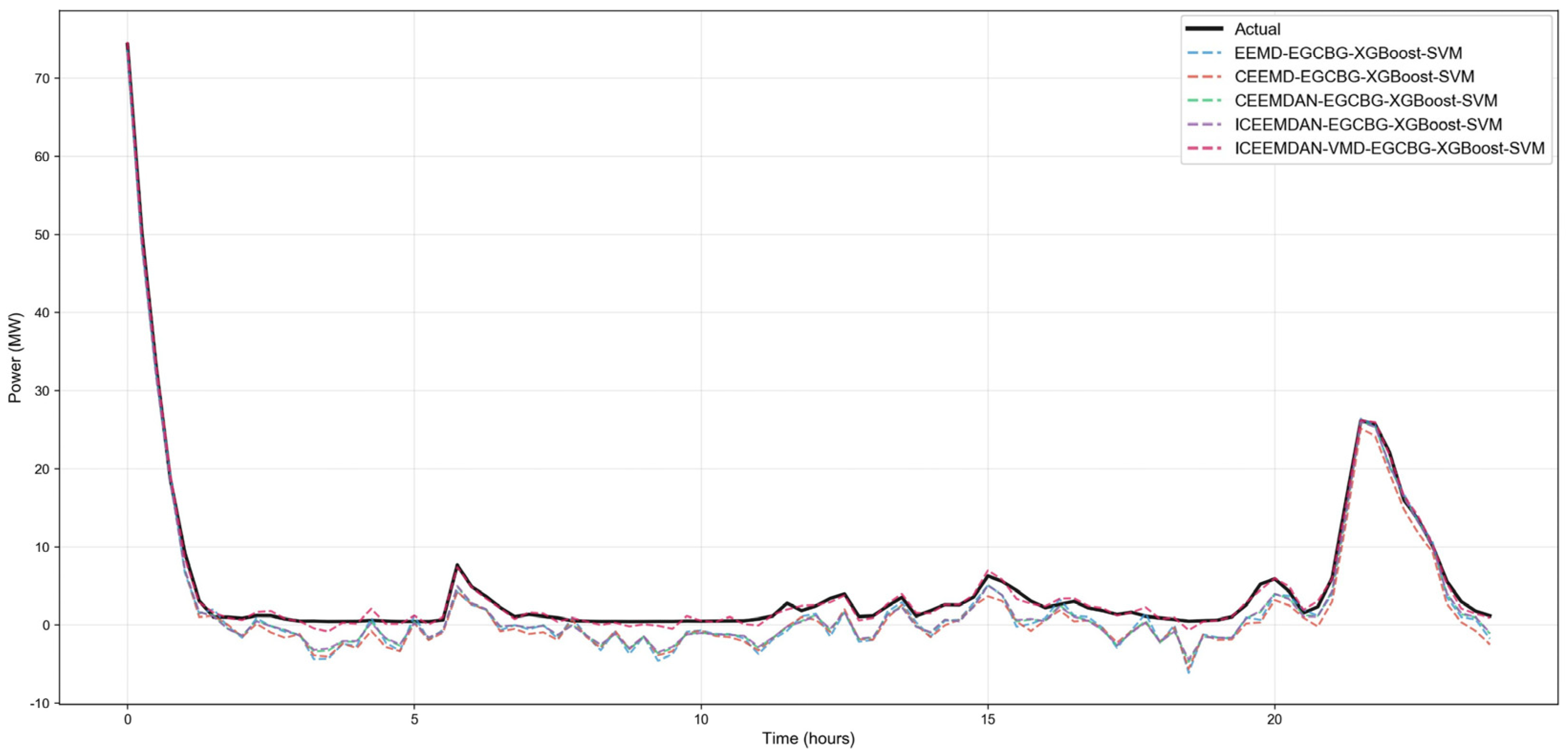
To make a more intuitive comparison of the fitting degree of each model, we plot the prediction curves for June 21st in Figure 11. The figure clearly shows that the model using the proposed ICEEMDAN-VMD quadratic decomposition algorithm is the closest to the actual power, thereby achieving the best prediction effect.

5. Conclusions

Under the “dual carbon” goal, improving wind power forecasting accuracy carries substantial importance. This paper introduces a multi-model fusion-based method for short-term wind power prediction, establishing a corresponding forecasting model to address the problem. The main research content is as follows:

Firstly, a wind power series decomposition and reconstruction method based on ICEEMDAN-VMD secondary decomposition is proposed, which uses ICEEMDAN to decompose the wind power data into several IMF subsequences, and divides these IMF subsequences into three different frequency components by combining Q statistics and sample entropy. Finally, VMD is used for secondary decomposition of high-frequency components, and the fluctuation features and residual noise of different scales are separated more finely. The medium- and low-frequency components that carry the main trend and main law are relatively stable and regular, and are directly retained or aggregated, avoiding unnecessary over-decomposition and calculation.

Secondly, the optimization algorithm GWO is improved by using the empirical exchange strategy EES, and the optimization performance of EES-GWO proposed in this paper is verified from three different perspectives by using 10 test functions ranging from simple to difficult. Through the exchange of experience between individuals, the diversity of the population is maintained, and the parameter space can be searched in a larger range, which significantly reduces the risk of falling into a local optimum. Moreover, experience sharing accelerates the dissemination of excellent information within the population, guides the population to approach the global optimal area faster and more accurately, achieves faster convergence and higher accuracy, and improves the stability of prediction.

This paper introduces a fusion model by synergizing an enhanced optimization algorithm and deep learning techniques. Because the trend of the mid- and low-frequency components obtained from the final decomposition in Section 2 is too moderate, in order to prevent overfitting, the XGBoost model is used to forecast the mid- and low-frequency components. Therefore, a multi-model fusion framework is explored. Within this framework, the forecasting results of all components are nonlinearly fused using the SVM model to generate the final results. Finally, the superiority and effectiveness of the proposed model in wind power prediction are verified by two examples. This paper uses wind power data from a wind power plant in Guohua Jingxia North Wind Power in Xinjiang Province in 2019, using a single wind farm’s data and regional climate characteristics, but it cannot reflect the evolution of large-scale weather systems (such as fronts and cyclones), and the prediction of sudden wind speed changes lags behind. It is easily disturbed by local measurement errors, wake effects, and terrain disturbances, and the generalization ability of the model is weak. Further research in this area will be considered in the future.

References

1. Huang, J.; Zhao, D.; Zhao, P. Review on technical pathways and assessment for carbon peaking and carbon neutrality in China’s building materials industry. Discov. Sustain. 2025, 6, 1188. [Google Scholar] [CrossRef] [Scilit]
2. Simões, T.; Tsami, M.; Nieto, F.; Huvaj, N. Renewable Energy Production in the Mediterranean: Exploring the Potential for Offshore Wind Development. IOP Conf. Ser. Earth Environ. Sci. 2025, 1552, 012012. [Google Scholar] [CrossRef] [Scilit]
3. Hassan, Q.; Algburi, S.; Sameen, A.Z.; Salman, H.M.; Jaszczur, M. A review of hybrid renewable energy systems: Solar and wind-powered solutions: Challenges, opportunities, and policy implications. Results Eng. 2023, 20, 101621. [Google Scholar] [CrossRef] [Scilit]
4. Chang, Y.; Yang, H.; Chen, Y.; Zhou, M.; Yang, H.; Wang, Y.; Zhang, Y. A Hybrid Model for Long-Term Wind Power Forecasting Utilizing NWP Subsequence Correction and Multi-Scale Deep Learning Regression Methods. IEEE Trans. Sustain. Energy 2024, 15, 263–275. [Google Scholar] [CrossRef] [Scilit]
5. Zhang, Y.; Wang, J.; Wang, X. Review on probabilistic forecasting of wind power generation. Renew. Sustain. Energy Rev. 2014, 32, 255–270. [Google Scholar] [CrossRef] [Scilit]
6. Kenmoé, G.D.; Fogno Fotso, H.R.; Aloyem Kazé, C.V. Comparative models for multi-step ahead wind speed forecasting applied for expected wind turbine power output prediction. Wind Eng. 2022, 46, 780–795. [Google Scholar] [CrossRef] [Scilit]
7. Wang, Y.; Wang, D.; Tang, Y. Clustered Hybrid Wind Power Prediction Model Based on ARMA, PSO-SVM, and Clustering Methods. IEEE Access 2020, 8, 17071–17079. [Google Scholar] [CrossRef] [Scilit]
8. Zhang, C.; Ma, H.; Hua, L.; Sun, W.; Shahzad, N.M.; Peng, T. An evolutionary deep learning model based on TVFEMD, improved sine cosine algorithm, CNN and BiLSTM for wind speed prediction. Energy 2022, 254, 124250. [Google Scholar] [CrossRef] [Scilit]
9. Sun, Y.; Zhou, Q.; Sun, L.; Sun, L.; Kang, J.; Li, H. CNN–LSTM–AM: A power prediction model for offshore wind turbines. Ocean Eng. 2024, 301, 117598. [Google Scholar] [CrossRef] [Scilit]
10. Zhang, J.; Sun, H.; Sun, Z.; Dong, W.; Dong, Y.; Gong, S. Reliability Assessment of Wind Power Converter Considering SCADA Multistate Parameters Prediction Using FP-Growth, WPT, K-Means and LSTM Network. IEEE Access 2020, 8, 84455–84466. [Google Scholar] [CrossRef] [Scilit]
11. Wang, J.; Niu, W.; Yang, Y. Wind turbine output power prediction by a segmented multivariate polynomial-XGBoost model. Energy Sources Part A 2024, 46, 505–521. [Google Scholar] [CrossRef] [Scilit]
12. Dong, X.; Miao, Z.; Li, Y.; Zhou, H.; Li, W. One data-driven vibration acceleration prediction method for offshore wind turbine structures based on extreme gradient boosting. Ocean Eng. 2024, 307, 118176. [Google Scholar] [CrossRef] [Scilit]
13. Wang, S.; Chang, L.; Liu, H.; Chang, Y.; Xue, Q. Short-term prediction of wind power based on temporal convolutional network and the informer model. IET Gener. Transm. Distrib. 2023, 18, 941–951. [Google Scholar] [CrossRef] [Scilit]
14. Ding, Y.; Chen, Z.; Zhang, H.; Wang, X.; Guo, Y. A short-term wind power prediction model based on CEEMD and WOA-KELM. Renew. Energy 2022, 189, 188–198. [Google Scholar] [CrossRef] [Scilit]
15. Liu, H.; Mi, X.W.; Li, Y.F. Wind speed forecasting method based on deep learning strategy using empirical wavelet transform, long short term memory neural network and Elman neural network. Energy Convers. Manag. 2018, 156, 498–514. [Google Scholar] [CrossRef] [Scilit]
16. Yang, S.; Yuan, A.; Yu, Z. A novel model based on CEEMDAN, IWOA, and LSTM for ultra-short-term wind power forecasting. Environ. Sci. Pollut. Res. 2022, 30, 11689–11705. [Google Scholar] [CrossRef] [Scilit] [PubMed]
17. Zhao, Z.; Nan, H.; Liu, Z.; Yu, Y. Multi-step interval prediction of ultra-short-term wind power based on CEEMDAN-FIG and CNN-BiLSTM. Environ. Sci. Pollut. Res. 2022, 29, 58097–58109. [Google Scholar] [CrossRef] [Scilit]
18. Hou, Z.; Bai, Y.; Ding, L.; Yue, X.; Huang, Y.; Song, W.; Bi, Q. Deep Learning Wind Power Prediction Model Based on Attention Mechanism-Based Convolutional Neural Network and Gated Recurrent Unit Neural Network. J. Circuits Syst. Comput. 2024, 33, 2450284. [Google Scholar] [CrossRef] [Scilit]
19. Peng, X.; Li, C.; Jia, S.; Zhou, L.; Wang, B.; Che, J. A short-term wind power prediction method based on deep learning and multistage ensemble algorithm. Wind Energy 2022, 25, 1610–1625. [Google Scholar] [CrossRef] [Scilit]
20. Sun, S.; Yu, P.; Xing, J.; Cheng, Y.; Yang, S.; Ai, Q. Short-Term Wind Power Prediction Based on ICEEMDAN-SE-LSTM Neural Network Model with Classifying Seasonal. Energy Eng. 2023, 120, 2761–2782. [Google Scholar] [CrossRef] [Scilit]
21. Sun, K.; Yang, D.; Wang, D.; Zhang, F. Development of a physics-guided bidirectional long short-term memory for wind power forecasting. Eng. Appl. Artif. Intell. 2026, 167, 113798. [Google Scholar] [CrossRef] [Scilit]
22. Jia, H.; Rao, H. Experience Exchange Strategy: An evolutionary strategy for meta-heuristic optimization algorithms. Swarm Evol. Comput. 2025, 98, 102082. [Google Scholar] [CrossRef] [Scilit]
23. Liu, S.; Sun, Z.; Sun, Y.; Kong, D. Short-term prediction of wind power based on grey wolf optimization Elman neural network algorithm. J. Phys. Conf. Ser. 2024, 2703, 012043. [Google Scholar] [CrossRef] [Scilit]
24. Zhang, H.; Wang, D.; Jiang, X. CrossGFA: Wind power prediction with a multi-scale cross-graph network via a Frequency-Enhanced Channel attention mechanism. Appl. Intell. 2025, 55, 48. [Google Scholar] [CrossRef] [Scilit]
25. Xu, X.; Zhou, X.; Fan, Q.; Yan, H.; Wang, F. A global attention based gated temporal convolutional network for machine remaining useful life prediction. Reliab. Eng. Syst. Saf. 2025, 260, 110997. [Google Scholar] [CrossRef] [Scilit]
Figure 1. Correlation analysis. (a) Pearson correlation analysis heatmap; (b) maximum mutual information coefficient heatmap.
Algorithms 19 00339 g001
Figure 2. Feature input analysis. (a) Wind speed–height correlation; (b) wind direction distribution; (c) correlation between wind speed and power; (d) meteorological factor correlation; (e) correlation in different wind speed intervals; (f) final selected features.
Algorithms 19 00339 g002
Figure 3. Population convergence comparison. Among them, the red dot and green star represent the population individual and the optimal individual respectively.
Algorithms 19 00339 g003
Figure 4. Prediction results of mid–low-frequency components in March. (a) Mid-frequency prediction; (b) mid-frequency error distribution; (c) low-frequency prediction; (d) low-frequency error distribution.
Algorithms 19 00339 g004
Figure 5. Fusion model structure diagram.
Algorithms 19 00339 g005
Figure 6. Original wind power sequence.
Algorithms 19 00339 g006
Figure 7. Decomposition process.
Algorithms 19 00339 g007
Figure 8. ICEEMDAN-VMD results.
Algorithms 19 00339 g008
Figure 9. Reconstruction error plots. (a) Reconstruction error comparison; (b) number of decomposed components; (c) reconstruction comparison.
Algorithms 19 00339 g009
Figure 10. Comparison of multiple model outputs. (a) Comparison of March prediction; (b) comparison of September prediction.
Algorithms 19 00339 g010
Figure 11. Prediction curve chart for June.
Algorithms 19 00339 g011