Enabling Reliable Industrial Energy Savings Verification Through Hybrid Factored Conditional Restricted Boltzmann Machine and Generative Adversarial Network

Abstract

Reliable quantification of industrial energy savings requires accurate detection of non-routine events (NREs) that distort post-retrofit baselines. Conventional statistical and rule-based anomaly detection methods often misinterpret operational variability, leading to biased or overstated savings under the International Performance Measurement and Verification Protocol (IPMVP). This study develops a novel IPMVP-compliant hybrid deep learning framework that integrates a deterministic Deep Neural Network (DNN) for baseline modeling with stochastic architectures, namely the Factored Conditional Restricted Boltzmann Machine (FCRBM) and Generative Adversarial Network (GAN), to capture probabilistic reconstruction patterns. Their outputs are fused using a hybrid thresholding mechanism that balances detection sensitivity and specificity. Using high-resolution data from an industrial glove manufacturing facility, the hybrid DNN–FCRBM model achieved the best trade-off, demonstrating an accuracy of 94.3%, a precision of 91.1%, and a low false positive rate of 5.1%. This model validated 11.32% industrial energy savings (approximately 478,050 kWh), equivalent to 237 tonnes of CO₂ avoided. The integration of stochastic generative learning within a deterministic framework strengthens transparency, auditability, and IPMVP compliance, offering a scalable pathway for credible industrial energy savings verification.

1. Introduction

Industrial facilities are frequently exposed to non-routine events (NREs) such as equipment breakdowns, sensor failures, and abrupt production shifts. These irregularities introduce anomalies into energy consumption data, distorting baseline models and undermining the accuracy of savings estimates in the reporting period. Such issues directly compromise the integrity of energy performance verification under the International Performance Measurement and Verification Protocol (IPMVP), where transparent and auditable reporting is essential. Despite their significance, anomalies are often treated in a generalised manner or omitted entirely from analysis, resulting in biased or unreliable savings assessments.

Traditional anomaly detection methods typically rely on static thresholds or rule-based logic, which struggle to differentiate between genuine anomalies and normal operational variability. This limitation leads to high rates of false positives and false negatives, reducing the credibility of reported savings. Moreover, conventional approaches often emphasise classification accuracy (e.g., F1-score, precision) without addressing the engineering-oriented requirements of IPMVP, such as uncertainty quantification and reproducibility. To address these shortcomings, recent studies have proposed hybrid approaches that combine statistical principles with machine learning [1]. Deep learning methods in particular have shown promise for high-dimensional, multivariate, and time-dependent industrial datasets, enabling more effective anomaly detection in complex and dynamic environments [2,3].

Beyond modelling, adaptive thresholding strategies have been developed to enhance sensitivity under varying power levels and operating conditions [4]. Other approaches, such as functional data clustering and non-intrusive monitoring, have been explored to improve interpretability and operational relevance in industrial systems [4,5]. Recent advances also include synthetic oversampling and feature selection to address class imbalance, which remains a key barrier to detecting rare but impactful events such as equipment breakdowns [6]. In parallel, explainable AI frameworks have emerged to support decision-making in cyber–physical systems, combining interpretability with robust detection capabilities [7,8,9]

Nevertheless, the integration of these methods within IPMVP-compliant M&V remains limited, especially in industrial contexts characterised by noisy, irregular, and large-scale datasets [10,11]. Current practices frequently lack transparency and traceability [12,13,14]. While deep learning architectures such as DNNs can capture complex nonlinear behaviour, they are often criticised as “black-box” models that offer limited interpretability and auditability—both essential for IPMVP compliance [15,16,17]. Similarly, many anomaly detection methods still rely on manually tuned static thresholds, which fail to adapt to operational variability and risk either overstating or underreporting savings [18]. Attempts at dynamic thresholding and ensemble optimisation remain underdeveloped and rarely deployed in industrial-scale applications [19,20,21].

These methodological gaps are particularly concerning given the increasing demand for verifiable energy savings in response to climate commitments, ESG frameworks, and national energy policies. International bodies, including the International Energy Agency (2022) [22], emphasise that industrial energy verification must align with the Paris Agreement and sustainability reporting standards. At the same time, industrial facilities generate vast, high-frequency datasets through advanced metering, building management systems, and IoT infrastructure, which exceed the capabilities of traditional spreadsheet-based or static M&V approaches [23,24]. While automated anomaly detection and predictive modelling are advancing, their integration into modular, scalable, and IPMVP-aligned workflows remains rare [25,26,27]. This gap limits adoption in performance-based contracting, investment-grade audits, and real-time savings verification [28].

Despite the growing application of deep learning in energy analytics, its integration into industrial Measurement and Verification (M&V) frameworks remains limited, particularly within the stringent requirements of the International Performance Measurement and Verification Protocol (IPMVP). Existing studies rarely address the dual challenge of anomaly interpretability and uncertainty quantification, which are critical for verifying real energy savings under complex and dynamic operating conditions. Furthermore, deterministic models such as Deep Neural Networks (DNNs) offer high predictive accuracy but fail to represent stochastic variability inherent in industrial processes, while generative models such as Factored Conditional Restricted Boltzmann Machines (FCRBM) and Generative Adversarial Networks (GAN) capture uncertainty but lack baseline alignment with engineering metrics.

To address these shortcomings, this study proposes an IPMVP-compliant hybrid deep learning framework that fuses deterministic and stochastic modelling through a hybrid thresholding mechanism based on reconstruction error statistics. The objectives are threefold: (1) to develop baseline energy prediction models using deterministic architectures for robust and auditable forecasting; (2) to enhance anomaly detection by integrating stochastic generative learning that captures contextual variability; and (3) to validate the framework through real industrial datasets, linking anomaly detection directly to measurable and verifiable energy savings.

The novelty of this research lies in its methodological synthesis of DNN and FCRBM/GAN models within a reconstruction error-driven hybrid threshold that aligns statistical learning with IPMVP uncertainty principles. It is hypothesised that this hybridisation improves anomaly detection accuracy, reduces false positives, and yields more credible post-retrofit savings estimates compared with traditional regression and standalone deep learning models. Through this approach, the study advances the field of industrial energy verification by bridging data-driven anomaly detection with transparent, policy-aligned decarbonisation practices.

2. Literature Review

2.1. The International Performance Measurement and Verification Protocol (IPMVP)

In industrial energy measurement and verification (M&V), traditional anomaly detection techniques have historically relied on statistical thresholds, rule-based logic, or regression-based residual analysis. While simple to implement, these methods are prone to misclassifying operational variability as anomalies, resulting in high rates of false positives or false negatives. This limitation reduces confidence in reported savings, particularly under the International Performance Measurement and Verification Protocol (IPMVP), which demands both accuracy and reproducibility [13,14,29]. Furthermore, static thresholding approaches are unable to adapt to dynamic industrial operating conditions, often leading to overstated or understated savings [18].

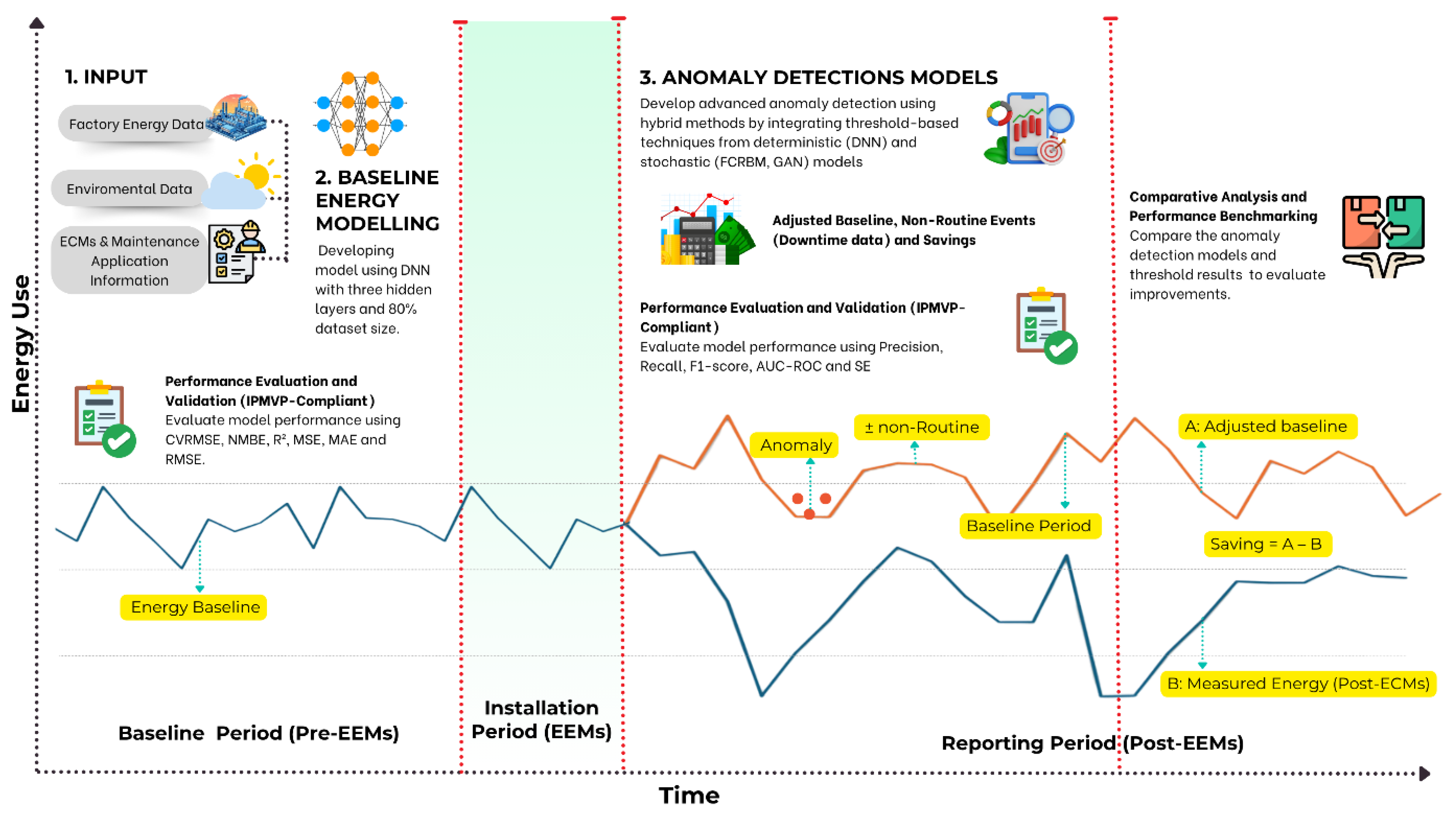
The International Performance Measurement and Verification Protocol (IPMVP) provides a structured framework for quantifying and verifying energy savings through four predefined options, namely Option A, Option B, Option C, and Option D, as summarised in

Table 1. Summary of IPMVP Options.

IPMVP Option	Analysis Approach	Common Use Cases
Option A: Retrofit Isolation Key Parameter Measurement	Engineering calculations with measured and stipulated data	Lighting upgrades; simple motor retrofits
Option B: Retrofit Isolation All Parameter Measurement	Engineering calculations based entirely on measured data	VFDs; chiller or HVAC component replacement
Option C: Whole Facility Measurement	Utility data analysis using comparison or regression methods	Envelope improvements; central plant upgrades
Option D: Calibrated Simulation	Computer simulation calibrated to actual performance	New buildings; major renovations

. Among these, Option C adopts a whole-facility approach, where energy savings are determined by comparing measured energy consumption during the reporting period against a statistically validated baseline model. In alignment with this framework, the present study adopts IPMVP Option C due to its suitability for industrial environments characterised by complex, high-frequency, and aggregated energy consumption data. This approach enables the evaluation of overall facility performance while accommodating multiple interacting energy efficiency measures (EEMs).

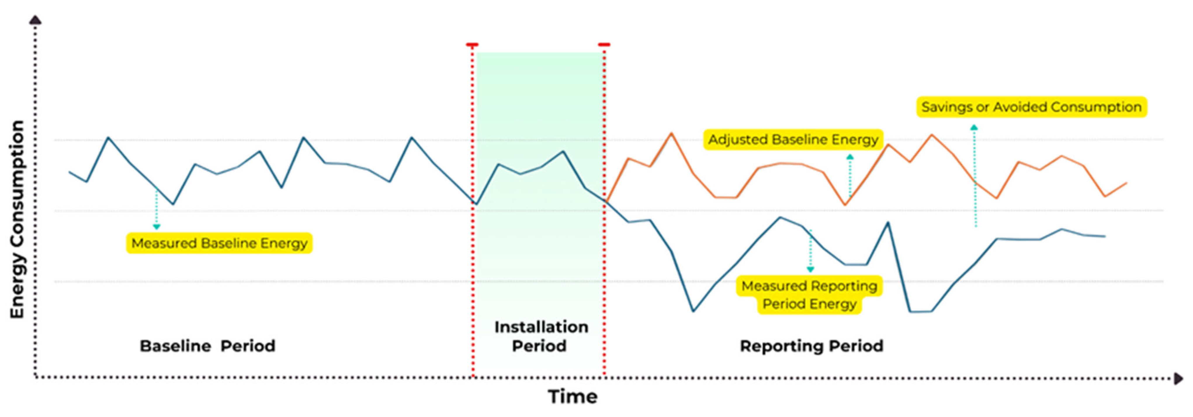
Figure 1 illustrates the fundamental structure of IPMVP-based verification through three key phases, namely the baseline period, installation period, and reporting period. During the baseline period, a reference energy model is established under normal operating conditions. In the reporting period, actual energy consumption is measured and compared with the adjusted baseline to quantify verified energy savings. In the figure, the blue line denotes measured energy consumption, whereas the orange line denotes the adjusted baseline energy during the reporting period. The shaded section indicates the installation period, and the gap between the adjusted baseline and the measured reporting period energy represents the verified savings or avoided consumption. To ensure compliance with IPMVP requirements, the baseline model must also satisfy the prescribed statistical validation criteria.

As summarised in

Table 2. Comparative Summary of Performance Metrics Across IPMVP Documents.

Metric	Primary Function	IPMVP 2022 [29]	Advanced M&V 2020 [31]	NRE/NRA Guide 2020 [30]	Established Thresholds/Guidance
CVRMSE	Accuracy of baseline model	Required	Referenced	Referenced	≤25% (hourly), ≤15% (monthly)
NMBE	Assessment of bias in baseline prediction	Required	Referenced	Referenced	≤10% (hourly), ≤5% (monthly)
Confidence Interval	Quantification of savings uncertainty	Required	Applied	Applied	95% confidence level recommended
Standard Error (SE)	Estimation precision	Supplementary metric	Applied	Applied	<50% of expected savings
R2	Goodness of regression fit	Mentioned	Applied	Mentioned	>0.75 acceptable; >0.9 considered excellent
FSU	Fractional savings uncertainty	Not specified	Key metric	Discussed	FSU < 50% at 68% confidence level
RMSE	Prediction error magnitude	Not specified	Frequently applied	Discussed	<5–10% of mean load (adjusted for autocorrelation)
MAE	Scale-free prediction accuracy	Not specified	Frequently applied	Discussed	≤5–7% of monthly average load
MSE	Error minimisation during model training	Not specified	Applied	Applied	No formal threshold; useful for model tuning
MAPE	Percentage-based error metric	Not specified	Occasionally referenced	Not referenced	Context-dependent; lacks formal threshold
Precision	Anomaly classification specificity	Not specified	Applied in classification	Applied (outlier analysis)	No universal threshold; supports model performance analysis
Recall	Sensitivity in detecting anomalies	Not specified	Applied	Mentioned	Supports anomaly/fault detection tasks
F1-Score	Harmonic mean of precision and recall	Not specified	Applied	Mentioned	Balanced metric for anomaly classification performance
AUC-ROC	Classifier performance under varying thresholds	Not specified	Applied in ML	Discussed	Evaluates trade-off between true and false positives; no formal threshold

, IPMVP Core Concepts (2022), IPMVP’s Snapshot on Advanced Measurement and Verification (2020), and the IPMVP Application Guide on Non-Routine Events and Adjustments (2020), all published by the Efficiency Valuation Organization (EVO) [30,31,32], mandate the use of CVRMSE and NMBE as primary indicators of model accuracy and bias. Confidence intervals are further recommended to quantify uncertainty in savings estimation. While additional metrics such as RMSE, MAE, and R² may enhance analytical rigour, they are considered supplementary and do not substitute the required IPMVP metrics.

Furthermore, the IPMVP Application Guide on Non-Routine Events emphasises the importance of identifying and accounting for operational deviations that may influence energy consumption. In industrial contexts, such deviations often manifest as anomalies arising from equipment breakdowns, production changes, or system disturbances. These events must be explicitly incorporated into baseline adjustment procedures to ensure that reported savings accurately reflect the impact of EEMs rather than external operational factors.

2.2. Machine Learning Approaches

To overcome these shortcomings, machine learning (ML) methods have been widely investigated for anomaly detection. Techniques such as support vector regression, clustering algorithms, decision trees, and k-nearest neighbours (K-NN) provide improved flexibility for modelling complex datasets with nonlinear and multivariate relationships. These methods have demonstrated effectiveness in industrial monitoring tasks, including condition-based maintenance and fault detection [20,21]. However, their application to IPMVP-compliant M&V remains limited due to challenges in handling high-dimensional time-series data and the lack of integration with engineering-focused performance metrics required for energy savings verification.

2.3. Deep Learning Methods for Anomaly Detection

Deep learning (DL) architectures have recently gained prominence for anomaly detection in industrial energy data. Models such as Deep Neural Networks (DNN), Convolutional Neural Networks (CNN), and Recurrent Neural Networks (RNN) can capture temporal dependencies and nonlinear behaviours across high-frequency datasets. They have been shown to improve anomaly detection performance in dynamic and complex environments [2,3]. Long Short-Term Memory (LSTM) networks, for instance, have been applied successfully to sequential energy data, enabling predictive modelling and anomaly detection with improved sensitivity. Despite their predictive power, these models are often regarded as “black boxes,” limiting interpretability and auditability, which are critical for compliance with IPMVP and stakeholder trust [16,17,33].

2.4. Hybrid Approaches and Thresholding Strategies

Hybrid approaches that combine statistical principles with advanced machine learning techniques have been proposed to address the weaknesses of standalone models. Ref. [34] demonstrated that combining statistical baselines with DL methods improves anomaly classification in industrial systems. Adaptive thresholding techniques have also been developed to account for variations in power levels and operating conditions, improving sensitivity to genuine anomalies [4]. Complementary strategies such as functional data clustering, non-intrusive load monitoring, and synthetic oversampling have been introduced to enhance interpretability, reduce class imbalance, and increase robustness in detecting rare events such as equipment breakdowns [5,6]. Nevertheless, these methods are rarely implemented in IPMVP-compliant M&V workflows, limiting their role in verified energy savings estimation. As summarised in

Table 3. Summary of Hybrid Deep Learning Models for Anomaly Detection in Energy Systems.

Model/Approach	Architecture	Application Context	Strengths	Limitations	Citation
WaDGN-AD	LSTM + GAN (Soft-DTW)	Energy time series with degradation cycles	Captures temporal dependencies effectively	Complex model; requires large datasets	[35]
Quantile RNN	RNN + Quantile Regression	Residential energy analysis	High accuracy; interpretable	Sensitive to threshold tuning	[36]
MENSA	Autoencoder + GAN + DNN	Smart grid cyberattack detection	Dual anomaly and attack detection	Protocol-specific; limited generalisation	[37]
Micro-Moment DNN	Rule-based + DNN	User behaviour in appliances	No labels needed; interpretable	Requires labelled features for training	[38]
DNN-GAN	1D-DCGAN + Soft-DTW	Building energy load forecasting	Improved parallel reconstruction	Overlapping sequences; unstable edge detection	[39]
Time-Series + CNN	Time-series + 2D CNN	Energy profile classification	Strong feature engineering	High computation demand	[40]
RBM + Free Energy	RBM	Anomaly detection in industrial energy	Captures hidden structures	Computationally intensive	[41]
RBM + Symbolic Dynamics	RBM + Symbolic Sequence Analysis	Symbol-based detection of deviations	Robustness and interpretability	Complex symbolic mapping setup	[41]
Hybrid Clustering	Unsupervised clustering + supervised learning	Baseline anomaly detection	Balanced accuracy with adaptive modelling	Requires threshold calibration	[42]
Autoencoder + SVR	Autoencoder + Support Vector Regression	Non-linear energy prediction	Effective for complex series	Requires feature selection	[43]
Improved K-NN	K-NN + Micro-Moment Features	Appliance anomaly detection	High sensitivity; few false alarms	Context-specific; window tuning required	[44]
Context-Aware DL	Context-aware deep learning	Smart grid and industrial systems	Promotes scalability	Dependent on context granularity	[45]
Proposed Framework (DNN–FCRBM Hybrid)	DNN + Factored Conditional RBM + reconstruction error thresholding	Industrial energy anomaly detection and IPMVP-compliant M&V	Balanced detection; low false positives; interpretable baseline adjustment; validated savings	Requires high-quality time-series data; computational training effort	This study

, recent frameworks demonstrate progress across diverse applications but often face challenges in adaptability, interpretability, or compliance with verification standards. The proposed DNN–FCRBM hybrid framework advances this landscape by explicitly aligning anomaly detection with IPMVP-compliant energy savings verification, ensuring both technical rigour and practical applicability in industrial environments.

2.5. Explainable and Interpretable Anomaly Detection

The increasing adoption of data-driven modelling has significantly enhanced anomaly detection capabilities within energy measurement and verification (M&V) frameworks. Nevertheless, several critical gaps persist, particularly in the context of industrial energy systems, as shown in Figure 1 below. Despite progress, few studies integrate deep learning-based anomaly detection into IPMVP-compliant M&V workflows. Most existing methods generalise anomaly types and lack focus on confirmed NREs. Additionally, probabilistic models like FCRBM remain underutilised, particularly in energy contexts. This study addresses these gaps by proposing a hybrid anomaly detection framework using DNN-FCRBM and DNN-GAN, guided by reconstruction error thresholds and validated against real industrial datasets. It aims to enhance interpretability, accuracy, and scalability in industrial M&V applications

2.6. Identified Gaps and Research Motivation

The literature demonstrates substantial progress in anomaly detection using machine learning and deep learning methods, yet critical gaps remain. Most existing models either prioritise generic classification accuracy over engineering precision or lack integration with IPMVP standards, resulting in limited transparency, reproducibility, and stakeholder confidence [10,11]. Furthermore, industrial-scale studies remain scarce, and existing frameworks often fail to handle operational noise, class imbalance, and real-world scalability. Finally, optimisation strategies such as dynamic thresholding and ensemble weighting remain underexplored in industrial energy contexts [19,21].

This study addresses these gaps by proposing a hybrid deep learning framework that integrates deterministic (DNN) and stochastic (FCRBM, GAN) models through a reconstruction error-based thresholding mechanism. The framework enhances anomaly detection accuracy, reduces false alarms, and enables IPMVP-compliant adjustment of baselines. By validating the method on high-resolution industrial data, this work advances the state of practice in M&V and provides a pathway for scalable, transparent, and verifiable energy savings verification.

3. Methodology

3.1. Methodological Framework

This study adopts an IPMVP-compliant framework, based on Option C, in which whole-facility energy savings are determined by comparing measured energy consumption during the reporting period with an adjusted baseline established from pre-implementation data. The overall structure of the study follows the standard IPMVP sequence of baseline period, installation period, and reporting period. As shown in Figure 2, the methodological framework links baseline modelling, anomaly detection, baseline adjustment, and savings verification within a single analytical procedure. To ensure consistent performance assessment throughout the study, the evaluation metrics used across all modelling stages are summarised in

Table 4. Key Performance Evaluation Metrics and Methods Recommended by IPMVP.

Category	Metric	Metric Full Name	Formula	Eq. *	IPMVP Criteria/ Recommended
Baseline Performance	CV RMSE	Coefficient of Variation of the Root Mean Squared Error	$\sqrt{{\displaystyle \frac{\frac{1}{N}{\sum }_{i=1}^N{\left(y_i-{\widehat{y}}_i\right)}^2}{\overline{Y}}}}\times 100\%$	(1)	Hourly: ≤25%, Monthly: ≤15%
	NMBE	Normalized Mean Bias Error	${\displaystyle \frac{{\sum }_{i=1}^N\left(y_i-{\widehat{y}}_i\right)}{\sum N_{i=1}{y}_i}}\times 100\%$	(2)	Hourly: ≤10%, Monthly: ≤5%
	R2	Coefficient of Determination	$R^2=1-{\displaystyle \frac{{\sum }_{i=1}^N{\left(y_i-{\widehat{y}}_i\right)}^2}{{\sum }_{i=1}^N{\left(y_i-\overline{Y_i}\right)}^2}}$	(3)	Not explicitly defined in IPMVP; higher values (closer to 1) are preferable. >0.9 (excellence), 0.75 < R < 0.9 (acceptable) Higher = better
	RMSE	Root Mean Squared Error	$\sqrt{{\displaystyle \frac{{\sum }_{i=1}^N{\left(y_i-{\widehat{y}}_i\right)}^2}{N}}}$	(4)	≤5–10% of mean load
	MBE	Mean Bias Error	${\displaystyle \frac{1}{N}}{\sum }_{i=1}^N{\left(y_i-{\widehat{y}}_i\right)}^2$	(5)	within ±5%
	MAE	Mean Absolute Error	${\displaystyle \frac{1}{N}}{\sum }_{i=1}^N{\left|y_i-{\widehat{y}}_i\right|}^2$	(6)	≤5–7% of monthly average load
	MSE	Mean Squared Error	${\displaystyle \frac{1}{N}}{\sum }_{i=1}^N{\left(y_i-{\widehat{y}}_i\right)}^2$	(7)	No specific threshold; used in AM&V tuning
	k-Fold CV	-	* N/A (Data split into 5 folds; performance evaluated across folds)	(8)	k = 5 (5-fold or 10-fold is most adopted).
Anomaly	Precision	-	${\displaystyle \frac{TP }{TP+FP}}$	(9)	≥0.90 for good anomaly detection
	Recall	-	${\displaystyle \frac{TP }{TP+FN}}$	(10)	≥0.85 for industrial fault detection
	F1-Score	-	$2\times {\displaystyle \frac{Precision\times Recall}{Precision+Recall}}$	(11)	≥0.85 for balanced classification models
	AUC-ROC	Area Under the Receiver Operating Characteristic Curve	${\int }_0^{1}TPR\left(t\right)dFPR\left(t\right)$	(12)	≥0.90 considered excellent model performance
Savings	RP	Relative Precision	$\sigma /\sqrt{n }$$\times$ t	(13)	RP ≤ 0.10 at 90% confidence

* N/A = not applicable; Eq. = equation.

. These include IPMVP-compliant baseline metrics such as CVRMSE and NMBE, together with supplementary measures including RMSE, MAE, MSE, R², precision, recall, F1 score, AUC ROC, and Relative Precision.

The inclusion of these metrics was supported by established protocols (IPMVP Core Concepts, 2022; IPMVP’s Snapshot on Advanced Measurement and Verification, 2020; IPMVP Application Guide on Non-Routine Events and Adjustments, 2020) [31,32,46] and literature [1,7,14], which recommend multiple error measures to capture distinct error characteristics.

The selection of these metrics was intended to ensure that each phase of the study was evaluated using criteria appropriate to its analytical objective. Baseline model validity was assessed primarily using CVRMSE and NMBE in accordance with IPMVP guidance, whereas anomaly detection performance was evaluated using precision, recall, F1 score, and AUC ROC. Savings reliability was subsequently assessed using Relative Precision, as defined in Equation (13). This integrated framework enables the study to maintain methodological consistency while extending conventional M&V practice through advanced data-driven anomaly detection.

3.2. Industrial Facility and Dataset

The study was conducted using operational data collected from a glove manufacturing facility in Malaysia operating under a continuous three-shift schedule. The industrial profile of the case facility is summarised in

Table 5. Industry Information.

Industry Attribute	Details
Location	Malaysia
Type of Industry	Healthcare
Product	Rubber glove
Raw Material	Synthetic latex
Energy Sources	Electricity
Type of Electricity Tariff	E2
Annual Energy Consumption	16,000,000.00 kWh
Operating hours (h)	24 h (3 shifts)
Data sources	SCADA, SEMS
Data dates	January 2021 until February 2023
EEMs	1. Chiller Optimisation (19–21 May 2022) 2. Scrubber optimisation (20 May 2022)

, which includes information on location, industry type, product, tariff category, annual electricity consumption, operating hours, data sources, monitoring period, and implemented energy efficiency measures. This industrial context is important because the facility exhibits complex multivariate energy behaviour that is strongly influenced by production activity, utility demand, and operational interruptions.

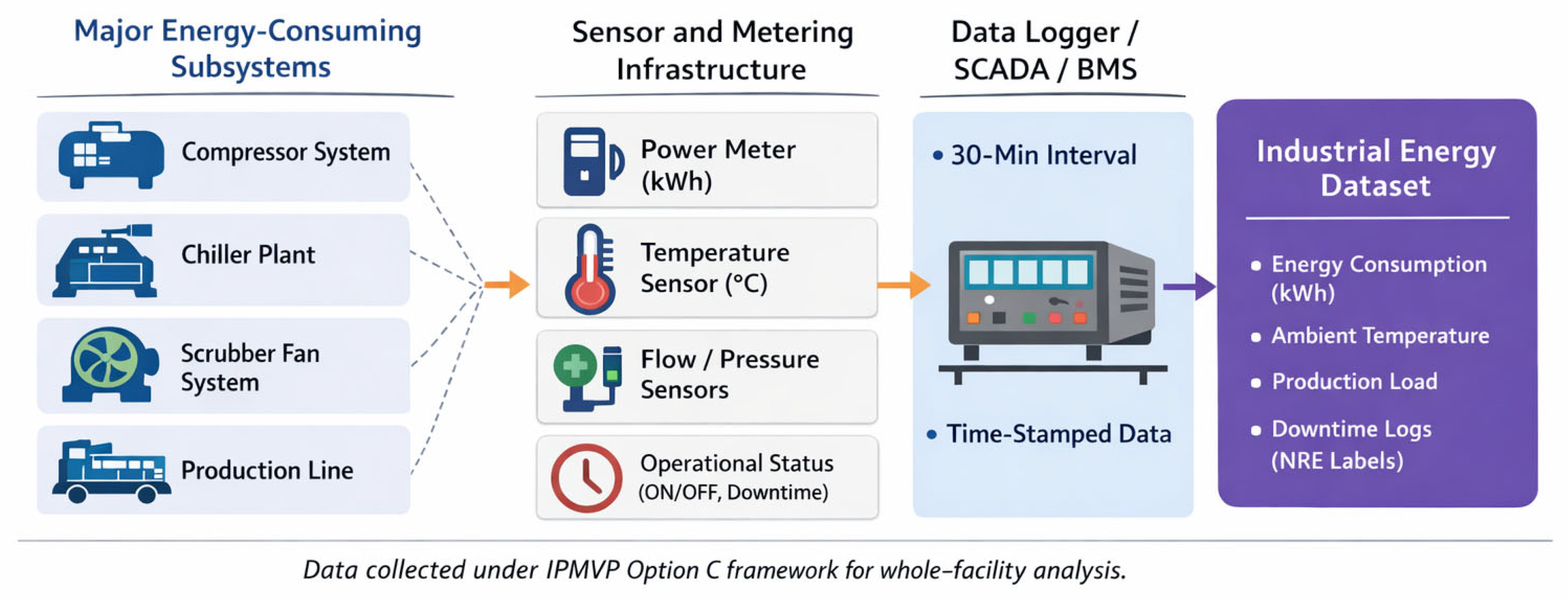
The monitored industrial system and data acquisition architecture are illustrated in Figure 3. The monitoring framework covers the primary energy-consuming subsystems of the facility, including compressors, chillers, scrubber fans, and production lines. Data were acquired through SCADA and SEMS platforms at 30 min intervals, thereby enabling the development of a high-resolution dataset suitable for baseline modelling and anomaly detection under the IPMVP Option C approach. The arrows in the figure indicate the flow of data from the monitored subsystems through the sensor and metering infrastructure to the data logger or SCADA/BMS platform, and subsequently to the industrial energy dataset. The combination of metered energy variables, operational indicators, environmental measurements, and downtime records provides the information necessary to represent both normal operating conditions and abnormal system behaviour.

The full list of monitored variables used in modelling is presented in

Table 6. Description of Monitored Variables and Their Role in Modelling.

Category	Variable	Description	Type	Service
Production Process	Production Line	Aggregate electricity demand associated with machines and operating units along the production line	Dependent	Process
	Line Speed	Operational speed of the production line, reflecting the rate of conveyor and line movement	Predictor	Process
	Product Output	Volume of completed products generated during the monitored time interval	Predictor	Production
	Product Weight	Average unit weight of products produced during manufacturing operation	Predictor	Production Quality
Equipment and Machine	Compressor	Combined electrical consumption of compressor units supporting plant operation	Predictor	Utility Process
	Chiller	Electricity demand of the chilled water generation and cooling system	Predictor	Utility Process
	Scrubber	Electrical usage of scrubber systems used for air or gas treatment	Predictor	Utility Process
	Compounding	Energy consumption attributed to the compounding stage of the manufacturing process	Predictor	Process
	Chemical Prep	Electricity demand associated with chemical preparation and mixing activities	Predictor	Process
	Bulk Tank	Electrical energy required for the operation and maintenance of bulk storage tanks	Predictor	Process
	IETS	Electricity consumed by the Integrated Effluent Treatment System during plant operation	Predictor	Support System
	Water Pump	Total electricity usage of pump systems involved in water circulation and supply	Predictor	Utility Process
Utility	Lighting	Facility-wide electrical consumption from lighting installations	Predictor	Building Services
	Others	Residual electricity demand not assigned to the main monitored equipment or process groups	Predictor	Building Services
Environmental	Outside Temperature	Ambient outdoor temperature surrounding the facility during operation	Predictor	Environmental Condition
	Visibility	External visibility condition representing atmospheric clarity in the surrounding area	Predictor	Environmental Condition
	Dew Point	Outdoor dew point temperature indicating moisture content in the air	Predictor	Environmental Condition
	Feels Like	Apparent outdoor temperature that combines thermal and atmospheric effects	Predictor	Environmental Condition
	Minimum Temperature	Lowest outdoor temperature recorded within the observation period	Predictor	Environmental Condition
	Maximum Temperature	Highest outdoor temperature recorded within the observation period	Predictor	Environmental Condition
	Pressure	Atmospheric pressure measured in the external plant environment	Predictor	Environmental Condition
	Humidity	Relative humidity level in the outdoor environment of the facility	Predictor	Environmental Condition
	Wind Speed	Measured speed of moving air outside the facility	Predictor	Environmental Condition
	Wind Degree	Direction of wind flow recorded in the external environment	Predictor	Environmental Condition
	Rain 1 h	Hourly rainfall quantity observed during the preceding one-hour period	Predictor	Environmental Condition
	Clouds All	Degree of cloud coverage in the outdoor atmosphere	Predictor	Environmental Condition
	Wind Gust	Peak short-duration wind intensity recorded in the surrounding area	Predictor	Environmental Condition

. These variables include production-related indicators, equipment-level electricity use, utility consumption, and weather-related predictors such as temperature, humidity, pressure, and wind characteristics. The dependent variable is the electricity consumption of the production line, while the remaining variables serve as predictors describing process, equipment, building, and environmental behaviour. The inclusion of this multivariate structure improves the ability of the models to capture nonlinear interactions between plant operation and facility-level energy demand.

To provide greater clarity on the role of downtime in anomaly detection, the recorded downtime events were further classified as either routine or non-routine. This classification helps to contextualise anomaly flags identified in the later analysis and ensures that observed energy deviations are interpreted in relation to actual plant conditions. As shown in

Table 7. Types of Downtime Events.

Issue	Remarks
Change Weight	Planned
Former Ratio, Change Product	Planned
Production Line/Tank Cleaning	Planned
Pump Coagulant/Latex	Planned
Breakdown	Unplanned
Robotic Arm Suspension Mechanism/Automated Suspension Mechanism Rectification	Unplanned, Mechanical Failure
Former (Cut Chain, Tensional Cart)	Unplanned, Mechanical Failure
Mechanical & Electrical Job	Unplanned, ADHOC
Production	Unplanned, ADHOC
Glove Tight Adjustment	Unplanned, Quality
Thickness Adjustment	Unplanned, Quality
Preventive Maintenance Operation Adjustment	Unplanned, Quality
Shortage	Shortage
No Order	Shortage

, routine activities represent expected operational interventions, whereas non-routine events include breakdowns, mechanical failures, ad hoc repair activities, and other unexpected disruptions. This categorisation forms the basis for linking detected anomalies to IPMVP-compliant baseline adjustment.

3.3. Data Processing and Feature Preparation

Prior to model development, a structured preprocessing procedure was applied to ensure data quality and analytical reliability. Exploratory data analysis was first performed to identify missing values, outliers, and the general statistical properties of the monitored variables. Variables with more than 30% missing values were excluded, while the remaining missing observations were imputed using cubic spline interpolation in order to preserve temporal continuity. Outliers were subsequently detected and removed using the interquartile range method. These preprocessing steps were necessary to minimise noise and prevent distorted learning behaviour during model training.

The pre-processed variables were then normalised using Z-score standardisation to ensure consistent feature scaling and to improve convergence during optimisation. In addition, multiple feature selection approaches were employed to reduce redundancy and strengthen model efficiency. The final dataset was divided into training, validation, and testing subsets using a 50:25:25 ratio. This data preparation stage provides the input foundation for the deterministic and stochastic models described in the subsequent sections, and its role within the complete analytical workflow is reflected in Figure 4.

3.4. Baseline Modelling and Benchmarking

A deterministic Deep Neural Network was first developed to establish the baseline model of expected facility energy consumption under normal operating conditions. The DNN learns the nonlinear relationship between whole-facility electricity use and the multivariate operational and environmental predictors described previously in Table 6. In parallel, a conventional ordinary least squares (OLS) linear regression model was implemented as an IPMVP-compliant benchmark. This reference model allows the proposed framework to be evaluated against a traditional baseline adjustment approach commonly used in measurement and verification practice.

The architecture and hyperparameter settings of the DNN, FCRBM, GAN, and hybrid models are summarised in

Table 8. Model Architecture and Hyperparameters.

Parameter	DNN	FCRBM	GAN	DNN-FCRBM	DNN-GAN
Layers	3 (64 units descending)	2 visible, 2 hidden	3 (Generator), 3 (Discriminator)	DNN + FCRBM layers	DNN + GAN layers
Activation	ReLU (hidden), Linear (output)	Sigmoid(visible) Binary (hidden)	LeakyReLU (G/D)	Same as DNN and FCRBM	Same as DNN and GAN
Training Algorithm	Adam Optimiser	Contrastive Divergence	Adversarial Training	Sequential training	Sequential training
Learning Rate	1.00 × 10−3	1.00 × 10−4	2 × 10−4 (G), 1 × 10−4 (D)	1 × 10−3 (DNN), 1 × 10−4 (FCRBM)	1 × 10−3 (DNN), 2 × 10−4 (GAN)
$\mathrm{k}$	3	3	3	3	3

. The DNN employed three hidden layers with ReLU activation and a linear output layer for energy prediction. The linear regression benchmark, by contrast, uses residual analysis and a fixed three sigma decision rule to identify anomalous observations. This comparison enables the study to assess the added value of hybrid deep learning approaches relative to a standard statistical reference model.

3.5. Hybrid Detection Architecture

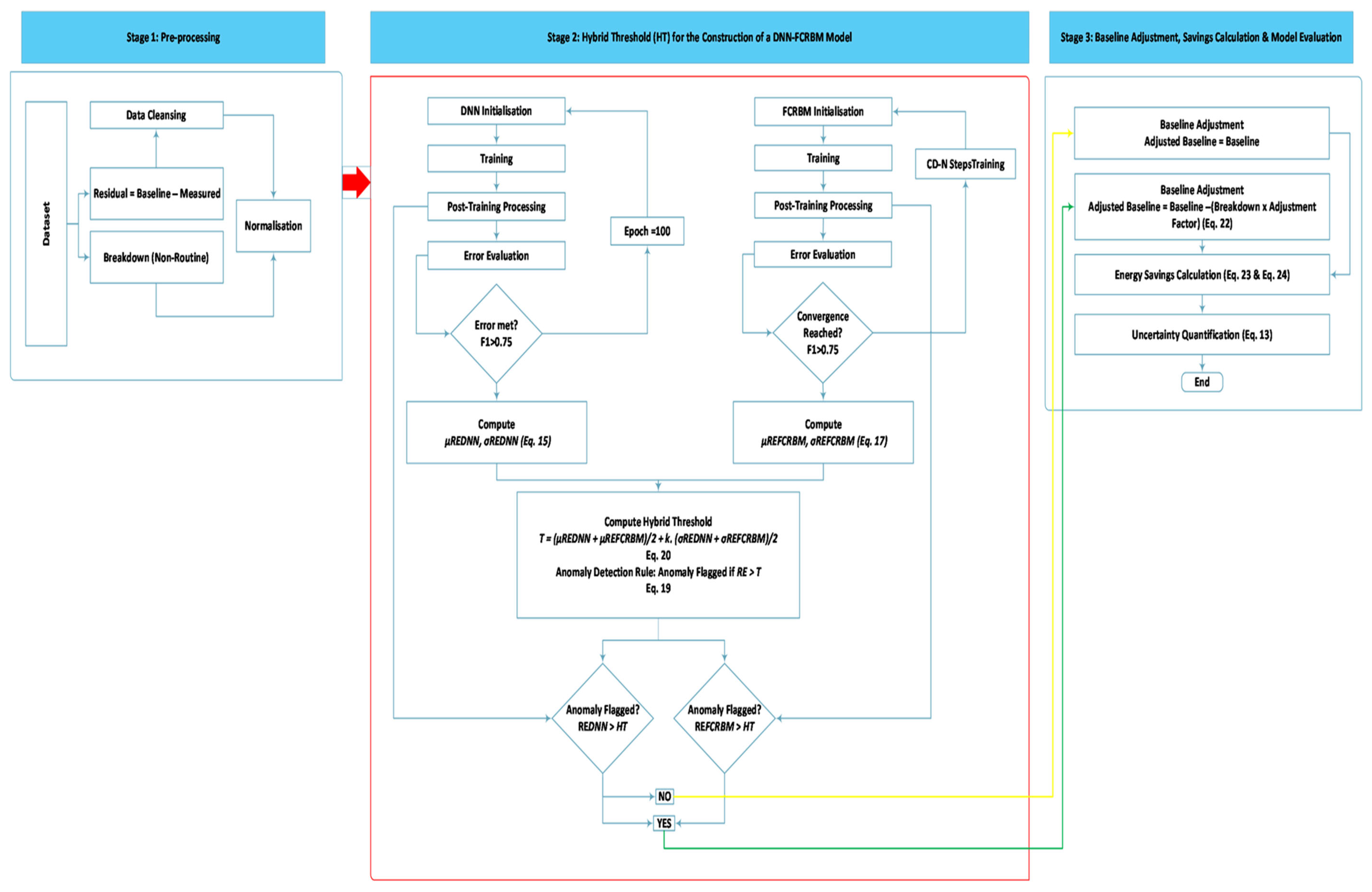
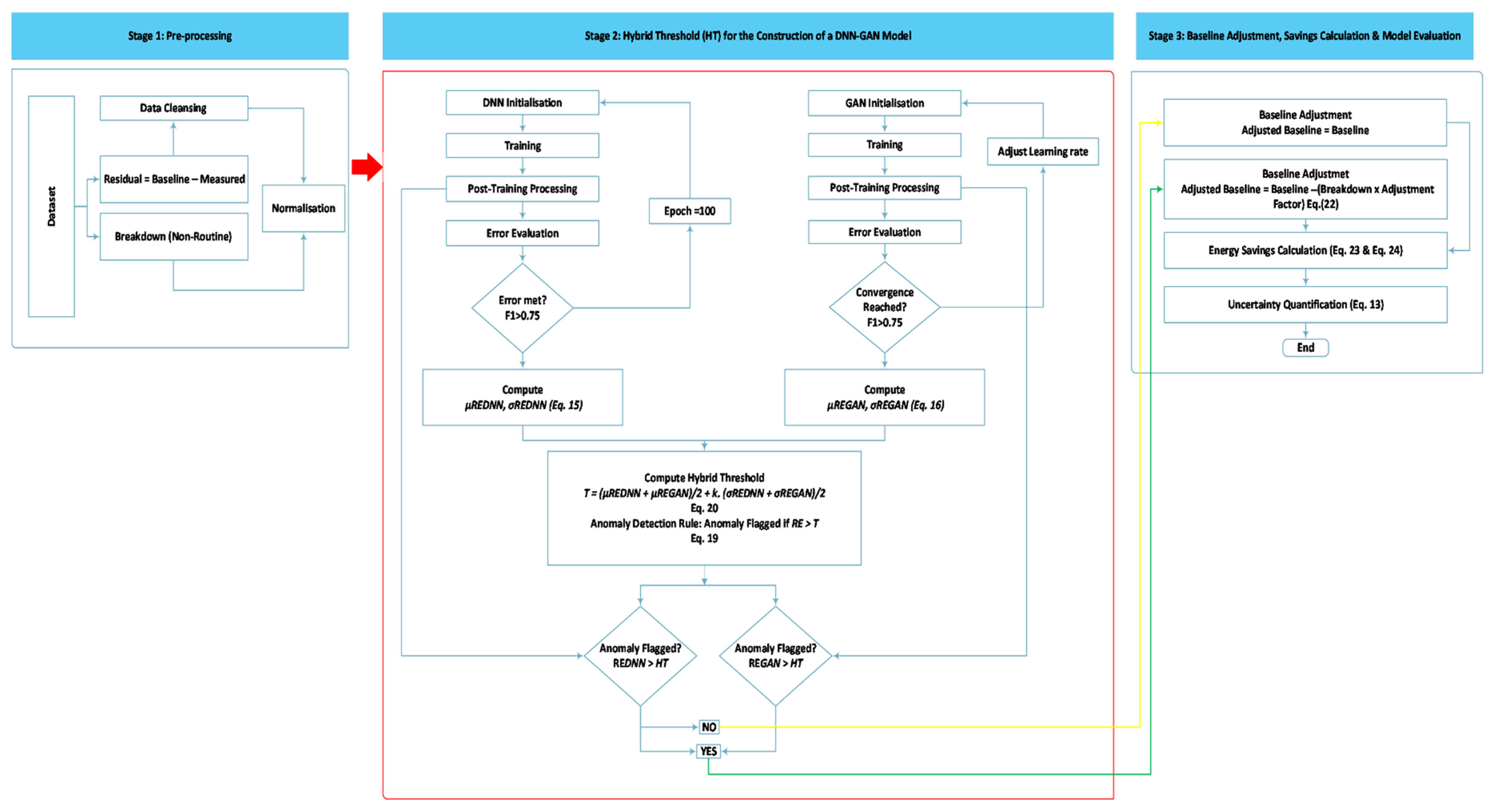
Two hybrid anomaly detection configurations were developed, namely DNN–FCRBM and DNN–GAN. The DNN–FCRBM workflow is illustrated in Figure 5, while the DNN–GAN workflow is shown in Figure 6. In both configurations, the DNN serves as the deterministic component that captures the expected baseline relationship between energy use and its explanatory variables. The stochastic component is then used to reconstruct system behaviour and quantify deviations through reconstruction error. This dual structure allows the framework to distinguish between normal operational variability and behaviour that is inconsistent with the learned energy patterns.

In the DNN–FCRBM configuration, the stochastic component is represented by the Factored Conditional Restricted Boltzmann Machine, which is trained using contrastive divergence to model temporal and contextual variability in facility operation. This configuration is particularly suitable for identifying physically meaningful deviations such as compressor instability, abnormal chiller loading, or intermittent process disturbances that may not be fully captured by deterministic baseline prediction alone. In the DNN–GAN configuration, the stochastic component is represented by a Generative Adversarial Network trained through adversarial optimisation. This approach improves sensitivity to subtle deviations and weak disturbances, although it may also increase the false positive rate due to its higher detection sensitivity. The overall relationship between deterministic baseline prediction, stochastic reconstruction, anomaly detection, and baseline adjustment is illustrated conceptually in Figure 4.

3.6. Anomaly Detection with Reconstruction Error

Anomaly detection in all deep learning configurations was based on reconstruction error. An observation was flagged as anomalous when its reconstruction error exceeded a predefined threshold, as defined in Equation (14). In this equation, the threshold is derived from the mean reconstruction error, the corresponding standard deviation, and a sensitivity factor. This formulation provides a consistent statistical decision rule for distinguishing normal and abnormal observations across all models.

The threshold formulation in Equation (14) is based on the residual-based statistical screening principle described in the IPMVP Application Guide on Non-Routine Events and Adjustments, where the mean and standard deviation of the data are used to identify observations that fall outside the expected range. In that guide, data exceeding approximately two to three standard deviations from the mean are treated as potential indicators of outliers or non-routine events by IPMVP Core Concepts (2022), IPMVP’s Snapshot on Advanced Measurement and Verification (2020), and the IPMVP Application Guide on Non-Routine Events and Adjustments (2020), all published by the Efficiency Valuation Organization (EVO) [31,32,46].

Equation (14) shows the general threshold for reconstruction error-based anomaly detection:

$$T={\mu }_{RE}+k·{\sigma }_{RE}$$

(14)

where

• ${\mu }_{RE}$ is the mean of the REs under normal conditions;
• ${\sigma }_{RE}$ is the Standard deviation of the reconstruction errors;
• $k$ represents the sensitivity factor.

Building on the general threshold in Equation (14), Equations (15)–(17) define the model-specific threshold formulations for DNN, FCRBM, and GAN, respectively. These equations retain the same statistical basis of mean and standard deviation, but are applied to the reconstruction error distributions generated by each model.

The model-specific forms of the reconstruction error threshold are given in Equations (15)–(17) for the DNN, FCRBM, and GAN models, respectively. These expressions allow each model to generate its own anomaly detection boundary according to its reconstruction behaviour. For the linear regression benchmark, anomaly detection followed the conventional three sigma rule based on residual deviation, as represented in Equation (18). This conventional threshold was included to provide a reference point for comparison with the adaptive reconstruction error thresholds used in the deep learning models.

Equation (15). DNN Reconstruction Error Threshold

$${\mu }_{R{E}_{DNN}}={\displaystyle \frac{1}{N}}\sum _{i=1}^{N}R{E}_{DNN}^{\left(i\right)},\hspace{1em}{\sigma }_{R{E}_{DNN}}=\sqrt{{\displaystyle \frac{1}{N}}\sum _{i=1}^N{\left(R{E}_{DNN}^{\left(i\right)}-{\mu }_{DNN}\right)}^2}$$

(15)

Equation (16). FCRBM Reconstruction Error Threshold

$${\mu }_{R{E}_{FCRBM}}={\displaystyle \frac{1}{N}}\sum _{i=1}^{N}R{E}_{FCRBM}^{\left(i\right)},\hspace{1em}{\sigma }_{R{E}_{FCRBM}}=\sqrt{{\displaystyle \frac{1}{N}}\sum _{i=1}^N{\left(R{E}_{FCRBM}^{\left(i\right)}-{\mu }_{R{E}_{FCRBM}}\right)}^2}$$

(16)

Equation (17). GAN Reconstruction Error Threshold

$${\mu }_{R{E}_{GAN}}={\displaystyle \frac{1}{N}}\sum _{i=1}^{N}R{E}_{GAN}^{\left(i\right)},\hspace{1em}{\sigma }_{R{E}_{GAN}}=\sqrt{{\displaystyle \frac{1}{N}}\sum _{i=1}^N{\left(R{E}_{GAN}^{\left(i\right)}-{\mu }_{R{E}_{GAN}}\right)}^2}$$

(17)

Equation (18). Linear Regression Residual Threshold

$${Threshold}_i=3\sigma$$

(18)

The anomaly decision rule itself is formalised in Equation (19), where a value of 1 indicates an anomalous observation and a value of 0 indicates normal operation. In practical terms, if the reconstruction error remains below the threshold, the observation is treated as normal because the model is able to reconstruct it satisfactorily. Conversely, if the reconstruction error exceeds the threshold, the observation is classified as anomalous because the model is unable to represent it within the learned normal pattern space. This rule is applied consistently across the single and hybrid model configurations.

Equation (19). Binary Anomaly Decision Rule

$$Anomaly Flag=\left\{\begin{array}{c} 1, Reconstruction Error \left(RE\right)>Threshold \left(T\right)\\ 0, Otherwise \\ \end{array}\right.$$

(19)

3.7. Hybrid Thresholding Strategy

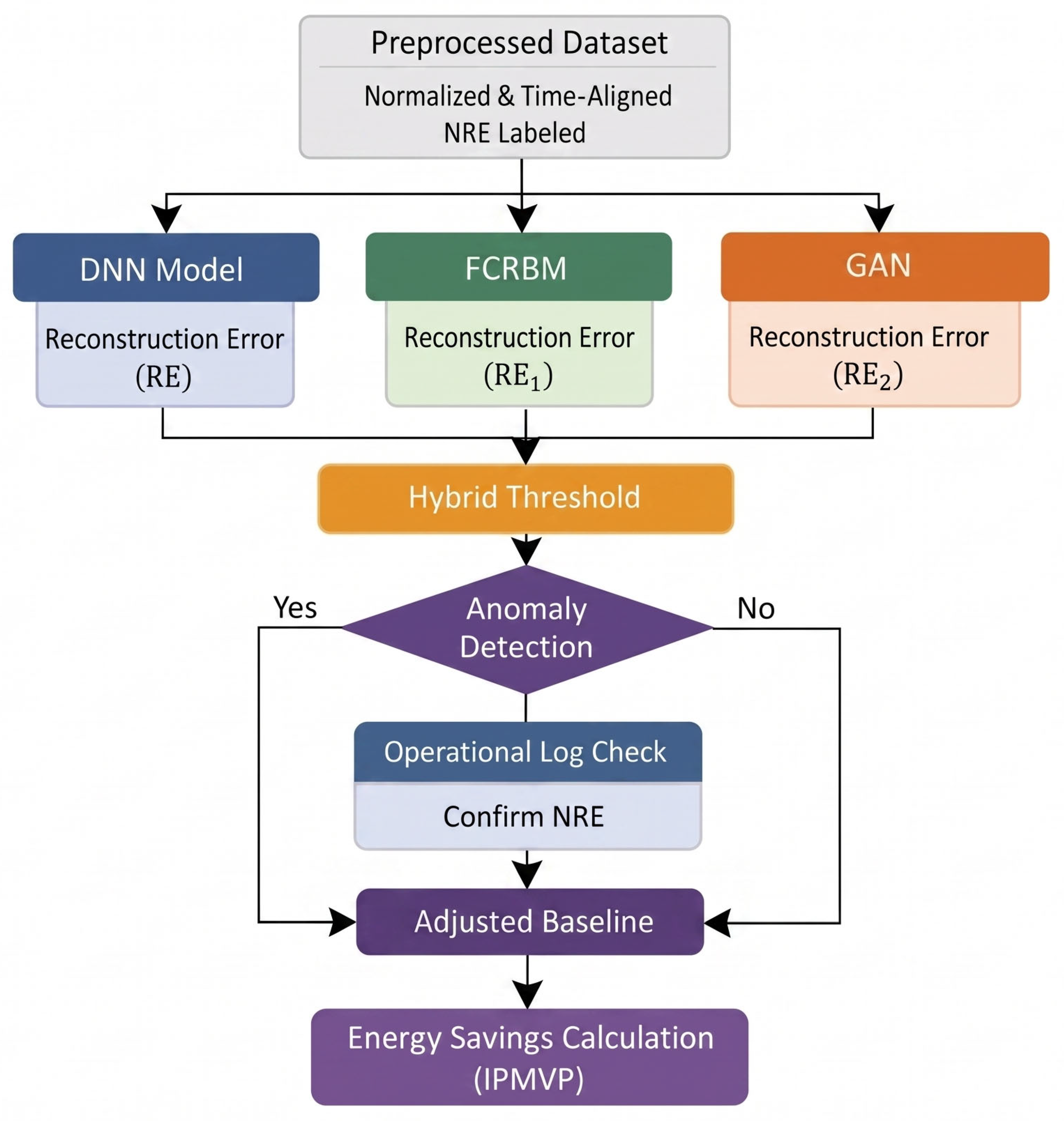
To improve anomaly detection reliability, the study introduces a hybrid thresholding strategy that combines the error statistics of two models at the decision level. This mechanism is central to the proposed DNN–FCRBM and DNN–GAN frameworks and is reflected in the workflows shown in Figure 5 and Figure 6. Rather than combining models at the feature level or structural level, the integration is performed by fusing their reconstruction error statistics into a single hybrid decision threshold.

The hybrid threshold is defined in Equation (20). This equation combines the mean reconstruction errors of the DNN and the secondary stochastic model with their corresponding standard deviations and a sensitivity parameter. The resulting threshold balances mean consensus and uncertainty averaging, thereby improving the trade-off between sensitivity and specificity. An anomaly is subsequently confirmed when the reconstruction error for a given observation exceeds the hybrid threshold, as expressed in Equation (21). Through this mechanism, deterministic feature learning from the DNN is integrated with probabilistic uncertainty representation from either the FCRBM or the GAN, producing a statistically robust decision boundary.

Equation (20) extends the residual-based thresholding principle into the hybrid formulation proposed in this study, where the average of the mean reconstruction errors from the deterministic DNN and the corresponding stochastic model represents the mean consensus component, and the average of their standard deviations represents the uncertainty averaging component. These components are combined to form a unified anomaly threshold. This formulation preserves the statistical logic of outlier screening while adapting it to the dual-model decision structure of the proposed framework.

Equation (20)—Hybrid Threshold Equation:

$$HT={\displaystyle \frac{{\mu }_{R{E}_{DNN}}+{\mu }_{R{E}_{M2}}}{2}}+k\left({\displaystyle \frac{{\sigma }_{R{E}_{DNN}}+{\sigma }_{R{E}_{M2}}}{2}}\right)$$

(20)

where

• ${\mu }_{R{E}_{DNN}}$ and ${\mu }_{R{E}_{M2}}$ are the mean reconstruction errors of the DNN and the secondary model, respectively;
• ${\sigma }_{R{E}_{DNN}}$ and ${\sigma }_{R{E}_{M2}}$ are their corresponding standard deviations;
• $k$ is the sensitivity factor;
• $M2$ refers to either the FCRBM or GAN model, depending on the hybrid combination.

Using this hybrid threshold, an observation is classified as anomalous when its reconstruction error exceeds the combined decision boundary defined in Equation (20), as formalised in Equation (21). This decision rule enables both deterministic and stochastic characteristics to be considered jointly during anomaly identification.

Equation (21)—Hybrid Anomaly Detection Condition:

$${Anomaly Flag}_i=\left\{\begin{array}{c}1, {RE}_i>HT\\ 0, Otherwise\end{array}\right.$$

(21)

where ${RE}_i$ is the reconstruction error for observation and $HT$ is the hybrid threshold.

The role of this hybrid thresholding mechanism within the full computational process is further illustrated in Figure 4, Figure 5 and Figure 6, which show how baseline prediction, stochastic reconstruction, anomaly detection, baseline adjustment, and energy savings verification are linked in one unified framework. This figure is especially important because it clarifies that anomaly detection does not operate as an isolated stage, but as an integral component of the IPMVP-compliant savings verification procedure.

3.8. Performance Evaluation Across the Analytical Phases

Model performance was evaluated in a phase-specific but internally consistent manner using the metrics defined earlier in Table 4. During baseline modelling, CVRMSE, NMBE, and R² were used as the primary criteria for assessing predictive validity, while RMSE, MAE, and MSE were used to provide additional information on bias, average error magnitude, and variance. During anomaly detection, precision, recall, F1 score, and AUC ROC were used to evaluate classification quality. During savings verification, Relative Precision was used to assess the reliability of the final energy savings estimates, as defined in Equation (13).

To further strengthen reproducibility and robustness, k-fold cross-validation was incorporated during model evaluation, as listed in Table 4. This was particularly important in assessing the stability of model performance across different data partitions and in reducing the risk of overfitting, especially in the deep learning configurations. Through this approach, all analytical stages remained connected to a common performance evaluation framework while still using metrics appropriate to the specific modelling objective of each stage.

3.9. Baseline Adjustment and Energy Savings Computation

Following anomaly detection, flagged observations were cross-referenced with downtime records and operational logs to determine whether they represented genuine non-routine events. Only anomalies that corresponded to confirmed NREs were used for baseline adjustment. This step is important because it prevents abnormal operational disturbances from being misinterpreted as energy savings. The baseline adjustment procedure therefore ensures that savings are attributed only to routine operational improvement and not to breakdowns, production disruption, or temporary plant malfunction.

The adjusted baseline for each confirmed anomalous period was computed using Equation (22), in which the original baseline prediction is modified using breakdown information and an adjustment factor. Verified interval level savings were then calculated using Equation (23) as the difference between the adjusted baseline and the measured energy consumption. Cumulative verified savings across the reporting period were subsequently obtained using Equation (24). Together, these equations form the mathematical basis of the savings verification stage under the proposed framework.

Equation (22)—Adjusted Baseline Equation:

$${\widehat{y}}_{i}adj={\widehat{y}}_i+\lambda di$$

(22)

where ${\widehat{y}}_i$ is the original baseline prediction, $di$ is the breakdown data, and λ is an adjustment factor.

Equation (23)—Interval Energy Savings Equation:

$$Si={\left({\widehat{y}}_i\right)}^{adj}-{\widehat{y}}_i$$

(23)

Equation (24)—Cumulative Energy Savings Equation:

$$S_{total}=i\sum S_i,\hspace{1em}S\%={\displaystyle \frac{S_{total}}{{\sum }_{i=1}^N{y}_i}}$$

(24)

This baseline adjustment and savings computation process is also conceptually aligned with the full modelling framework shown in Figure 6, where anomaly detection outputs are passed forward into the baseline adjustment stage before final savings verification. Accordingly, the proposed methodology preserves transparency, reproducibility, and auditability while extending traditional M&V practice through adaptive anomaly-informed baseline correction. Building on this methodological framework, Section 4 evaluates the performance of the proposed approach by first comparing it with the conventional IPMVP baseline model before examining the anomaly detection and savings verification results in greater detail.

4. Result and Discussion

4.1. Comparison with Conventional IPMVP Baseline Model

To evaluate the proposed framework against established measurement and verification practice, the hybrid deep learning models were benchmarked against a conventional baseline model based on linear regression using the ordinary least squares method. Linear regression remains widely used in IPMVP Option C applications because of its simplicity, transparency, and ease of interpretation. As such, it provides an appropriate reference model for assessing the extent to which the proposed hybrid framework improves anomaly detection and savings verification under dynamic industrial operating conditions.

The linear regression model describes the relationship between energy consumption and its influencing variables through the prediction function given in Equation (25), while the corresponding residuals were computed using Equation (26) as the difference between observed and predicted energy values. In accordance with conventional IPMVP-based statistical thresholding practice, anomaly detection was performed using a three-sigma criterion, where observations with residuals exceeding ±3σ standard deviations were classified as potential non-routine events.

Equation (25)—Linear Regression Prediction Model:

$$Y_{predict}=b_0+b_1{X}_1+b_2{X}_2+\dots {+b}_p{X}_p$$

(25)

where $Y_{predict}$ is the predicted energy consumption; $b_0$ is the intercept; $b_1$, $b_2\dots \dots .,b_p$ and $X_1,X_2$,……., $X_p$ are the slope coefficients for each independent variable.

Equation (26)—Residual Calculation:

$$Residual=Y_{predict,i}-Y_{actuai,i}$$

(26)

where $Y_i$ represents the actual observed value, and $Y_{predict,i}$ is the predicted value from the model.

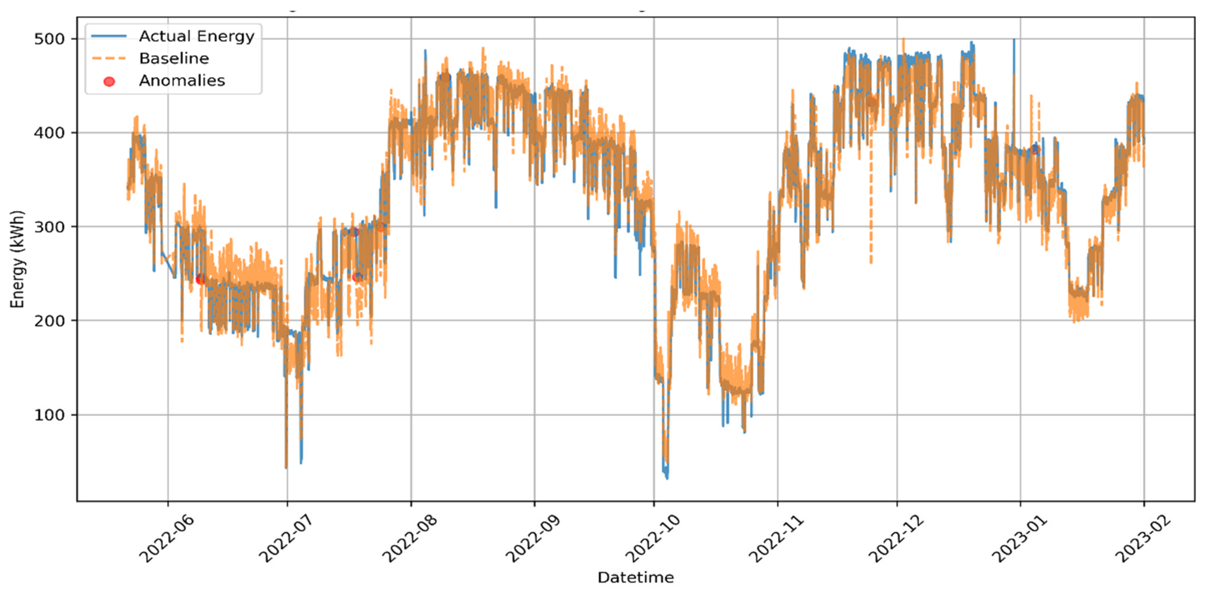
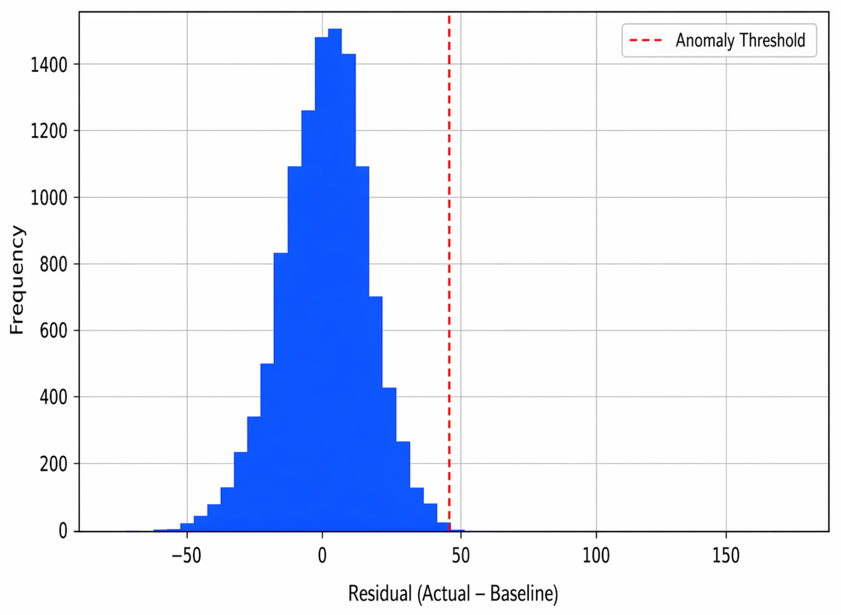
The anomaly detection summary obtained from the linear regression benchmark is presented in

Table 9. Linear Regression Anomaly Detection Summary.

Threshold Factor (k)	Standard Deviation (σ)	Threshold (T)	Total Anomalies Detected
3 (99.73% Confidence)	15.16 kWh	45.47	8 cases

, which shows that only a limited number of anomalies were identified under the statistical thresholding approach. This behaviour is further illustrated in Figure 7, where the detected anomalies appear as isolated deviations from the predicted baseline. In parallel, the residual distribution shown in Figure 8 indicates that although the linear regression model captures the general energy trend, it remains constrained by its linear assumptions and fixed statistical threshold, which reduce its ability to identify transient, nonlinear, and context-dependent anomalies.

Despite these limitations in anomaly detection, the baseline prediction performance of the linear regression model remained within acceptable IPMVP validation limits. As reported in

Table 10. Model Evaluation Summary for Baseline Prediction under IPMVP Framework.

Metric	Value	IPMVP Compliance Status
NMBE	0.13	Within IPMVP limits
CVRMSE	4.47	Within IPMVP limits
R2	0.9643	High model accuracy (R2 > 0.9)
MAE	4.89	Informative only
MBE	2.15	Informative only
Standard Deviation	15.39	Informative only

, the model achieved compliant CVRMSE and NMBE values, together with a high coefficient of determination. This confirms that the linear regression benchmark provides a statistically valid and IPMVP-compliant baseline model, thereby ensuring that the comparison with the proposed hybrid models is both fair and methodologically consistent.

A more detailed examination of the detected anomalies is provided in

Table 11. Analysis of Energy Anomalies as Non-Routine Events.

Date Time	Anomaly (kWh)	Threshold	Downtime	NREs	Adjusted Baseline
2022-06-09 10:00:00	49.9098	45.4691	8.0	YES	YES
2022-06-09 10:30:00	56.8322	45.4691	7.5	YES	YES
2022-07-17 17:00:00	46.0016	45.4691	3.5	YES	YES
2022-07-18 14:30:00	51.3060	45.4691	3.5	YES	YES
2022-07-24 10:00:00	52.1951	45.4691	3.0	YES	YES
2022-08-09 17:00:00	87.4110	45.4691	2.0	YES	YES
2022-11-24 12:00:00	173.9746	45.4691	0	NO	NO
2023-01-04 13:00:00	45.8114	45.4691	3.0	YES	YES

, which links residual exceedances with downtime events and their classification as non-routine events. The results show that not all statistically detected anomalies correspond to actual operational disruptions. This finding highlights a key limitation of conventional threshold-based detection, namely that statistical exceedance alone is insufficient to distinguish between genuine NREs and normal process variability. In practical terms, this limitation may lead either to missed disturbances or to insufficient baseline adjustment during savings verification.

Overall, the linear regression benchmark demonstrates that conventional IPMVP-compliant methods remain useful for basic anomaly screening and baseline validation. However, their reliance on linear relationships and fixed thresholds limits their effectiveness in complex industrial environments characterised by nonlinear behaviour, intermittent disturbances, and operational variability. This limitation provides the basis for the subsequent evaluation of the proposed hybrid deep learning models, which utilise reconstruction error-based thresholding to improve anomaly sensitivity and contextual discrimination.

4.2. Comparative Performance of Deep Learning Models

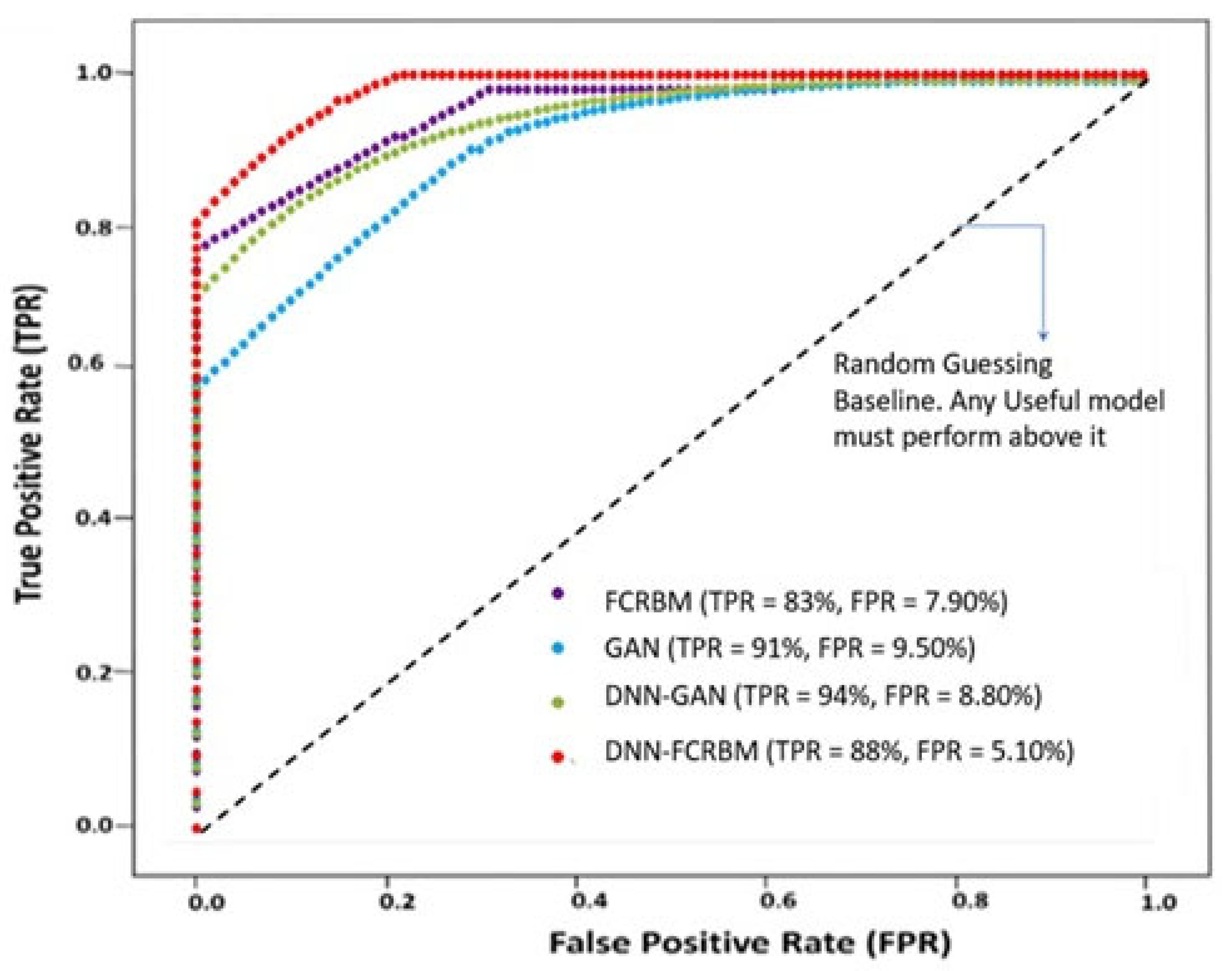
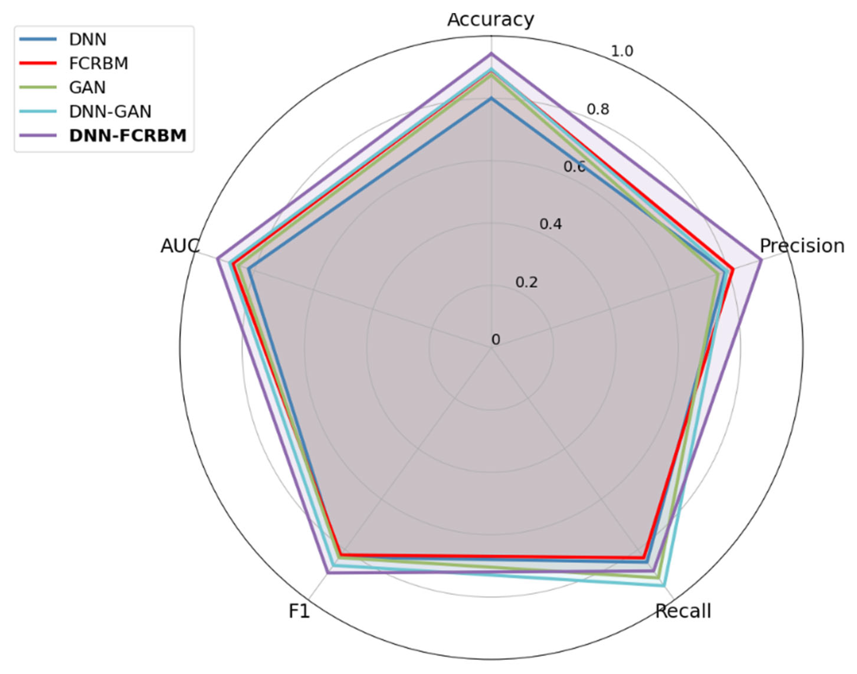
Five deep-learning-based models, namely DNN, FCRBM, GAN, DNN–FCRBM, and DNN–GAN, were trained and evaluated using identical datasets. As summarised in

Table 12. Performance Analysis.

Method	Accuracy	Precision	Recall	F1	AUC	TPR	FPR
FCRBM	0.8912	0.8156	0.8327	0.8219	0.8728	83%	7.90%
GAN	0.8745	0.7652	0.9124	0.8321	0.8547	91%	9.50%
DNN-FCRBM	0.9428	0.9113	0.8854	0.8927	0.9246	88%	5.10%
DNN-GAN	0.8934	0.7951	0.9438	0.8629	0.8835	94%	8.80%

, DNN–FCRBM achieved the highest overall accuracy (0.943), F1-score (0.893), and the lowest false-positive rate (5.1%), whereas DNN–GAN recorded the highest recall (0.944) but with a comparatively larger false-positive rate (8.8%). The ROC curves further support these findings, with DNN–FCRBM producing the largest enclosed area under the curve (AUC = 0.925), indicating superior discrimination between normal and abnormal operating states. This improved balance between sensitivity and specificity can be attributed to the complementary learning roles of the deterministic and stochastic components, in which the DNN captures the average operational behaviour while the FCRBM reconstructs probabilistic deviations around that baseline. Statistical significance testing using a two-sample t-test (p < 0.05) further confirmed that the improvement in accuracy and precision achieved by the hybrid model over the standalone DNN was not random, but reflects a genuine methodological gain.

To facilitate clearer comparison across models, the quantitative values reported in Table 12 were used directly to generate Figure 9. Thus, Figure 9 serves as the visual representation of the same performance metrics presented in Table 12, rather than as an independent result. As shown in Figure 9, the comparative profile of accuracy, precision, recall, and F1-score confirms that DNN–FCRBM provides the most balanced overall performance, while DNN–GAN achieves higher recall at the expense of more false positives. This consistency between the tabulated values and the graphical visualisation strengthens the robustness and transparency of the reported comparison.

To further examine the discriminative capability of the models, Figure 10 presents the Receiver Operating Characteristic (ROC) curves for the FCRBM, GAN, DNN–FCRBM, and DNN–GAN models. The figure shows that DNN–FCRBM encloses the largest area under the curve (AUC = 0.925), confirming its superior ability to distinguish between normal and abnormal operating states. This observation is consistent with the quantitative results reported in Table 12 and further strengthens the conclusion that the DNN–FCRBM configuration provides the most robust overall anomaly detection performance among the evaluated models.

4.3. Reconstruction Error and Threshold Sensitivity

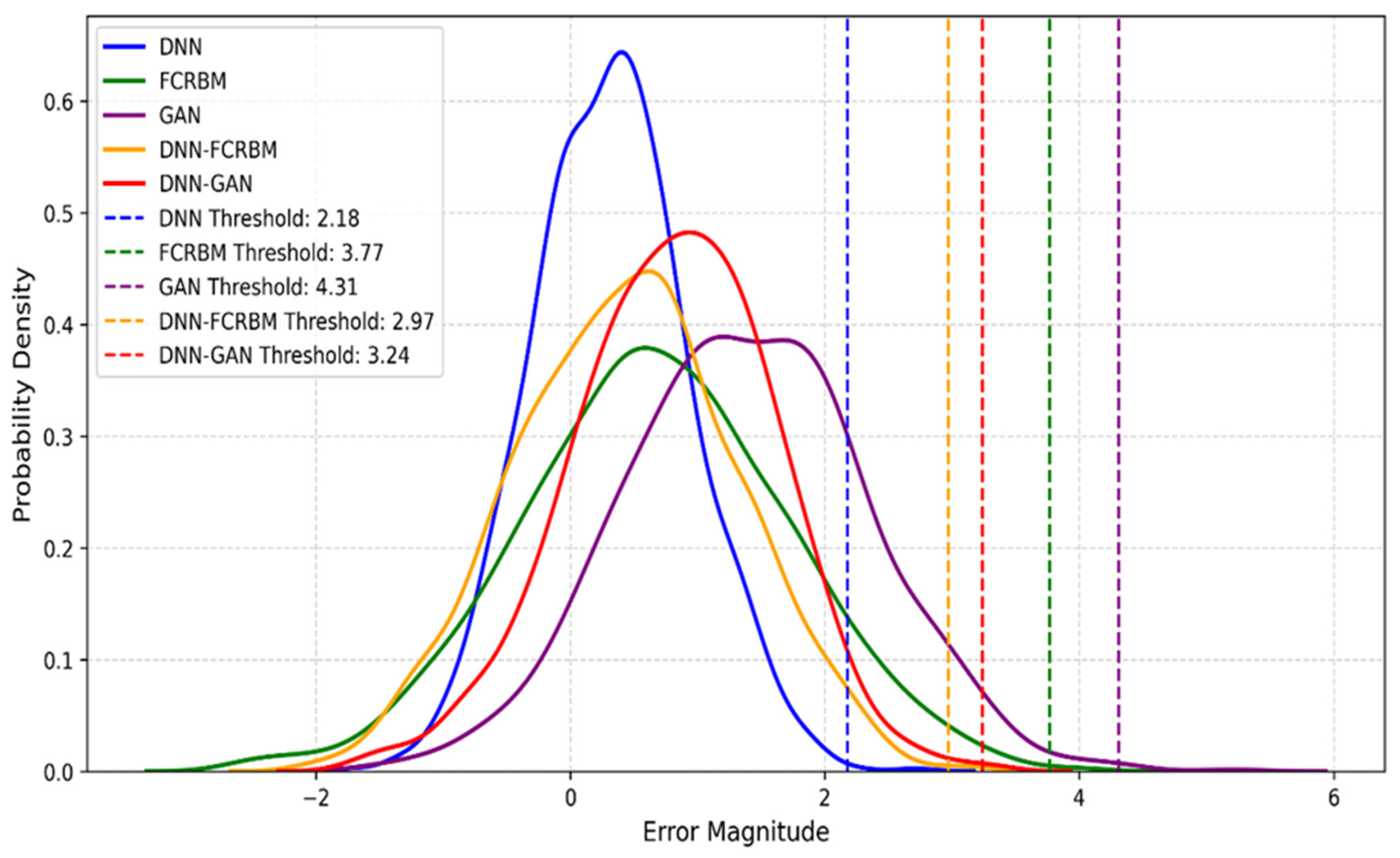
Figure 11 and

Table 13. Summary of Mean and Standard Deviation of Reconstruction Errors for Different Models.

Method	$\mathbf{Mean} \left(\mathsf{\mu }\right)$ RE	$\mathbf{SD} \left(\mathsf{\sigma }\right)$ RE
LR	-	15.1615
DNN	0.3102	0.6231
FCRBM	0.5848	1.0614
GAN	1.3765	0.9772
DNN-FCRBM	0.4475	0.8423
DNN-GAN	0.8434	0.8002

show the probability density of reconstruction errors. The DNN and DNN–FCRBM models yielded the smallest mean errors (0.31 and 0.45) and lowest standard deviations (0.62 and 0.84). In contrast, GAN-based models exhibited wider error distributions (mean > 0.8) and higher variance, implying weaker convergence and higher sensitivity to noise.

The hybrid threshold mechanism dynamically weighted the mean and standard-deviation components of the deterministic and stochastic errors, producing adaptive detection boundaries that minimised both missed detections and false alarms. Sensitivity analysis on the weighting parameter α (0.2 ≤ α ≤ 0.8) showed optimal stability at α ≈ 0.5, where the hybrid model achieved maximum F1-score with minimal fluctuation in recall and precision. This confirms that balanced weighting between deterministic and stochastic components yields robust detection under variable industrial conditions.

Anomaly Detection Patterns and Interpretation

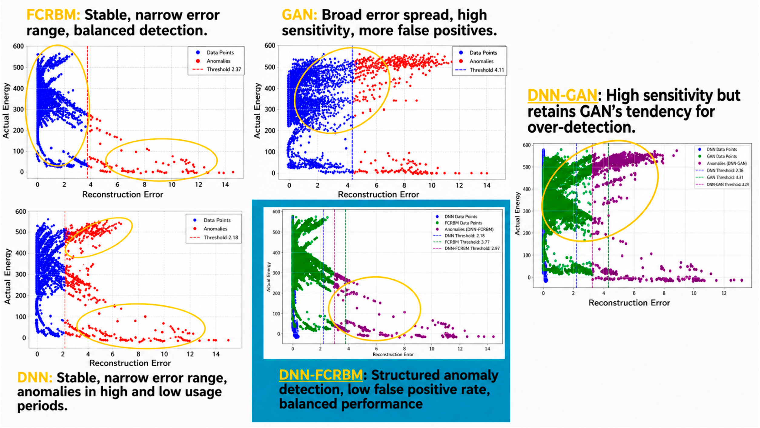
Visual examination of the detection scatter plots in Figure 12 reveals distinct clustering patterns among the models. In the individual model plots, the coloured points represent normal data points and detected anomalies as indicated in each panel legend, while the dashed vertical lines denote the anomaly thresholds. In the hybrid model plots, different colours are used to distinguish the outputs of the component models and their corresponding anomaly points. DNN and FCRBM anomalies are concentrated around operational transitions, indicating sensitivity to production-level fluctuations. GAN-based detections are more dispersed, suggesting higher responsiveness but also greater sensitivity to transient noise. The hybrid models display more bounded anomaly clusters aligning with recorded downtime intervals, demonstrating improved contextual detection of genuine non-routine events. This visual behaviour supports the quantitative results, showing that DNN-FCRBM more effectively isolates physically meaningful anomalies while reducing spurious detections.

4.4. Impact on Energy Savings Verification

All deep learning models complied with IPMVP precision limits (RP < 0.01), but the verified savings magnitude varied with detection accuracy (

Table 14. Anomaly Detection and Savings.

Method	Threshold	Number of Anomalies Detected	Confirmed Non- Routine Events (NREs)	Percentage of NREs (from 14,433 Entries Points)	Total Energy Savings (kWh)	Percentage Savings	RP
LR	45.48	8	7	0.05%	650,579.42	15.40%	0.1262
DNN	2.18	2251	179	1.25%	458,362.41	10.85%	0.0052
FCRBM	3.77	3079	209	1.45%	473,332.52	11.21%	0.0088
GAN	4.31	3223	249	1.73%	465,147.37	11.01%	0.0081
DNN-FCRBM	2.97	4210	857	5.94%	478,050.01	11.32%	0.0070
DNN-GAN	3.24	4894	1320	9.12%	400,697.69	10.71%	0.0067

Note: DNN-FCRBM. Provides the best trade-off between anomaly detection accuracy, saving realism and statistical reliability.

).

• Linear regression: 650,579 kWh (15.4%)—overstated due to under-detection of anomalies.
• DNN: 458,362 kWh (10.85%).
• FCRBM: 473,333 kWh (11.21%).
• GAN: 465,147 kWh (11.01%).
• DNN–FCRBM: 478,050 kWh (11.32%).
• DNN–GAN: 400,698 kWh (10.71%).

The DNN–FCRBM result corresponds to 237 tonnes of CO₂ avoided, confirming both environmental and economic significance. The close proximity of DNN, FCRBM, and DNN–FCRBM results indicates convergence toward realistic savings once anomalies are properly filtered, whereas the inflated regression estimate illustrates the cost of relying on static thresholds.

From an engineering perspective, this demonstrates that the hybrid framework prevents false savings attribution, improving audit credibility and supporting investment-grade verification.

To provide greater clarity on the role of downtime in anomaly detection, the recorded downtime events were first classified as either routine or non-routine. This classification helps to contextualise the anomaly flags identified in the subsequent analysis, ensuring that observed energy deviations are interpreted in relation to actual operational conditions. The summary of this classification is presented in

Table 15. Types of Downtime Events and NRE Classification.

Issue	Remarks	Classification
Change in weight	Planned	Routine
Ratio or product change	Planned	Routine
Line/tank cleaning	Planned	Routine
Pump or latex coagulant maintenance	Planned	Routine
Breakdown	Unplanned	NRE
Robotic arm suspension failure	Unplanned, Mechanical	NRE
Former (cut chain, tensional cart)	Unplanned, Mechanical	NRE
Mechanical & electrical jobs	Unplanned, Ad hoc	NRE
Production interruptions	Unplanned, Ad hoc	NRE

.

This categorisation distinguishes planned operational activities from unplanned disruptions. Routine activities refer to scheduled or expected interventions, whereas non-routine events (NREs) represent unexpected deviations such as breakdowns, mechanical failures, or ad hoc repairs. As such, Table 15 establishes the basis for interpreting the anomaly detection results discussed in the following sections.

Building on this classification,

Table 16. Worked Example (Weekly Energy Data with Anomalies and Adjusted Baseline (August 2022)).

Date	Predicted Baseline (kWh)	Measured Energy (kWh)	Residual (kWh)	Anomaly Flag	NRE Confirmed	Adjusted Baseline (kWh)	Savings (kWh)
2022-08-01	12,540.0	12,410.5	−129.5	No	–	12,540.0	129.5
2022-08-02	12,520.0	12,830.7	+310.7	Yes	Yes	12,831.0	0.3
2022-08-03	12,530.0	12,510.2	−19.8	No	–	12,530.0	19.8
2022-08-04	12,600.0	12,950.1	+350.1	Yes	No	12,600.0	0.0
2022-08-05	12,550.0	12,460.4	−89.6	No	–	12,550.0	89.6
Total	–	–	–	–	–	–	239.2

presents a worked example for one representative week in August 2022 to further illustrate how anomaly detection influences baseline adjustment and verified savings. The table compares measured energy consumption with the predicted baseline, identifies anomalous observations, and demonstrates how confirmed NREs lead to adjustments in the baseline and, consequently, the resulting savings.

This example shows that anomalies confirmed as NREs (e.g., 2022-08-02) are incorporated into the adjusted baseline, effectively nullifying the savings for that day. In contrast, anomalies not validated as NREs (e.g., 4 August) are excluded, preserving the original baseline and ensuring that routine fluctuations do not distort savings. This case study demonstrates the operational credibility of the DNN-FCRBM framework, where baseline adjustments are directly tied to validated NREs.

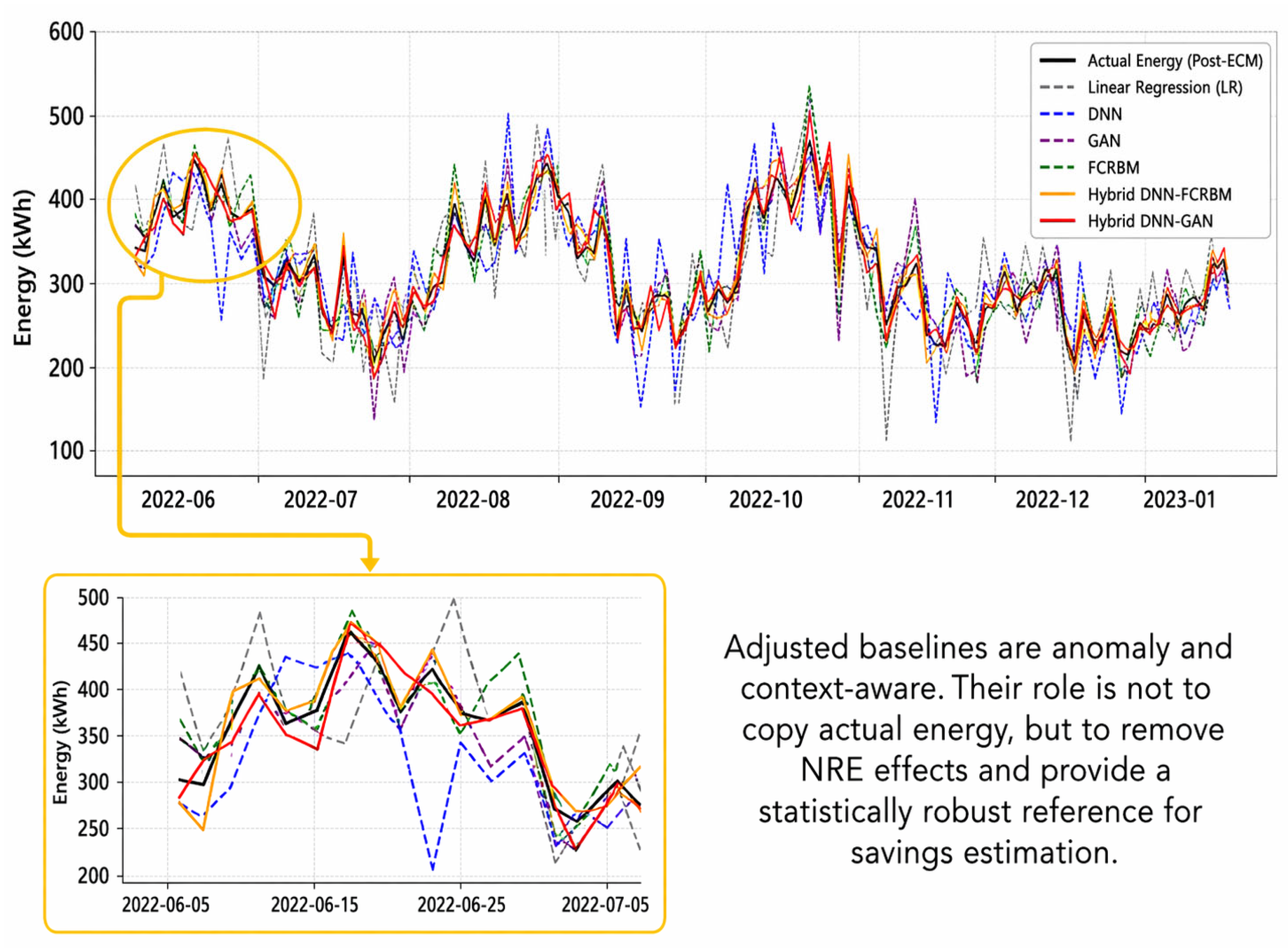
Figure 13 illustrates how differences in anomaly detection behaviour across models translated into distinct adjusted baselines, directly impacting the magnitude of reported energy savings. The comparison underscores that reliable anomaly detection is not only a technical requirement but also central to ensuring transparency and auditability in industrial energy performance verification.

The robustness of the proposed framework under varying conditions is supported by both the dataset characteristics and the modelling approach. The dataset spans an extended monitoring period and includes environmental variables such as temperature, humidity, and pressure, which enable the model to capture variations associated with seasonal changes. In addition, operational variability is represented through different categories of industrial activities and downtime events, as summarised in Table 15, which includes both planned operations (e.g., production changes, cleaning, and maintenance) and unplanned disruptions (e.g., breakdowns and mechanical failures). These variations reflect realistic and dynamic operating conditions within the industrial facility.

Furthermore, the incorporation of anomaly detection and non-routine event (NRE) based baseline adjustment allows the model to adapt to operational disturbances. By distinguishing between normal variations and actual disruptions, the framework ensures that changes in operating conditions do not distort energy savings estimation. Overall, these elements demonstrate that the proposed model is capable of handling both seasonal variability and operational changes within the evaluated industrial context.

Key Insights and Final Considerations

The comparative analysis demonstrates that DNN–FCRBM provides the most balanced combination of accuracy, precision, recall, and interpretability, making it the most reliable model for industrial anomaly detection within an IPMVP-compliant framework. Compared with conventional regression-based detection, which identified only a limited number of anomalies and risked overstating savings, the hybrid model captured a broader range of non-routine events while maintaining statistical robustness.

Although DNN–GAN achieved higher recall, its higher false positive rate reduced its suitability for practical M&V deployment. By contrast, DNN–FCRBM produced more stable reconstruction error behaviour, resulting in fewer false alarms and more credible baseline adjustment. This finding underscores the importance of balancing sensitivity with reliability in industrial environments, where excessive false positives may distort reported savings and weaken operational confidence.

A major contribution of this study is the hybrid thresholding mechanism, which integrates deterministic and stochastic modelling into a unified anomaly detection strategy. Applied to real industrial data from a glove manufacturing facility, the framework verified 11.32% energy savings, equivalent to 478,050 kWh and 237 tonnes of CO₂ avoided. Although the validation was conducted on a single facility, the results demonstrate strong potential for transparent, auditable, and scalable energy savings verification in complex industrial settings.

5. Conclusions

This study introduced a robust, IPMVP-compliant framework for industrial energy performance verification that integrates advanced baseline modelling with hybrid deep learning-based anomaly detection. By combining deterministic (DNN) and stochastic (FCRBM, GAN) models through a novel hybrid thresholding mechanism, the framework effectively overcomes the limitations of traditional thresholding and accurately identifies non-routine events (NREs). Among the tested configurations, the DNN–FCRBM consistently offered the best balance between accuracy, precision, and false positive control, establishing it as the most reliable model for practical M&V deployment. The framework was successfully validated on real industrial data from a glove manufacturing facility and confirmed 11.32% energy savings (≈478,050 kWh, 237 tonnes CO₂ avoided). Although the proposed framework demonstrated robust performance within the studied industrial setting, the present evaluation was conducted on a single industrial facility. Accordingly, broader generalisation to other sectors and facilities should be interpreted with caution, and future work should include validation across multiple plants with diverse operating characteristics and process conditions. Although the proposed hybrid framework is more computationally demanding than conventional statistical models, its intended deployment is based on interval-level industrial monitoring rather than ultra-low-latency control. Since the monitored data are acquired at 30 min intervals, the principal computational burden lies in offline model training, whereas operational deployment involves applying the trained models to periodic incoming data for anomaly screening and savings verification. Although seasonality was not isolated as a separate experimental factor, the framework was evaluated using long-duration, high-resolution industrial data spanning diverse environmental conditions, operating states, and downtime scenarios, supporting its robustness within the studied industrial context. Overall, these findings demonstrate that the proposed end-to-end pipeline offers a scalable, auditable, and transparent approach to energy savings estimation, directly linking anomaly detection to actionable, verifiable energy impact in line with industrial decarbonisation objectives.

References

1. Pan, H.; Yin, Z.; Jiang, X. High-Dimensional Energy Consumption Anomaly Detection: A Deep Learning-Based Method for Detecting Anomalies. Energies 2022, 15, 6139. [Google Scholar] [CrossRef] [Scilit]
2. Garg, A.; Zhang, W.; Samaran, J.; Savitha, R.; Foo, C.-S. An Evaluation of Anomaly Detection and Diagnosis in Multivariate Time Series. IEEE Trans. Neural Netw. Learn. Syst. 2022, 33, 2508–2517. [Google Scholar] [CrossRef] [Scilit]
3. Nizam, H.; Zafar, S.; Lv, Z.; Wang, F.; Hu, X. Real-Time Deep Anomaly Detection Framework for Multivariate Time-Series Data in Industrial IoT. IEEE Sens. J. 2022, 22, 22836–22849. [Google Scholar] [CrossRef] [Scilit]
4. Pan, G.; Qian, J.; Ouyang, J.; Luo, Y.; Wang, H. Adaptive Threshold Event Detection Method Based on Standard Deviation. Meas. Sci. Technol. 2023, 34, 075903. [Google Scholar] [CrossRef] [Scilit]
5. Bermeo-Ayerbe, M.A.; Ocampo-Martinez, C.; Diaz-Rozo, J. Non-Intrusive Condition Monitoring Based on Event Detection and Functional Data Clustering. Eng. Appl. Artif. Intell. 2023, 124, 106625. [Google Scholar] [CrossRef] [Scilit]
6. Malarselvi, G. A Multifaceted Approach for Enhancing Anomaly Detection in Industrial Systems with Adaptive Synthetic Sampling and Machine Learning Evaluation. J. Electr. Syst. 2024, 25, 2124–2131. [Google Scholar] [CrossRef] [Scilit]
7. Mendia, I.; Gil-Lopez, S.; Grau, I.; Del Ser, J. A Novel Approach for the Detection of Anomalous Energy Consumption Patterns in Industrial Cyber-Physical Systems. Expert Syst. Appl. 2024, 41, e12959. [Google Scholar] [CrossRef] [Scilit]
8. Wadinger, M.; Kvasnica, M. Adaptable and Interpretable Framework for Anomaly Detection in SCADA-Based Industrial Systems. Expert Syst. Appl. 2024, 246, 123200. [Google Scholar] [CrossRef] [Scilit]
9. Hillenbrand, J.; Gönnheimer, P.; Gerlitz, E.; Fleischer, J. Design and Implementation of a Holistic Framework for Data Integration in Industrial Machine and Sensor Networks. Procedia CIRP 2021, 104, 1771–1776. [Google Scholar] [CrossRef] [Scilit]
10. Ahern, M.; O’Sullivan, D.; Bruton, K. Development of a Framework to Aid the Transition from Reactive to Proactive Maintenance Approaches to Enable Energy Reduction. Appl. Sci. 2022, 12, 6704. [Google Scholar] [CrossRef] [Scilit]
11. Md Adnan, W.N.W.; Dahlan, N.Y.; Musirin, I. Artificial Neural Network Optimization in Prediction Baseline Energy Consumption to Quantify Energy Savings in Commercial Building. In IEEE Control and System Graduate Research Colloquium (ICSGRC); IEEE: New York, NY, USA, 2020; pp. 393–397. [Google Scholar] [CrossRef] [Scilit]
12. Gallagher, C.V.; Bruton, K.; Leahy, K.; O’Sullivan, D.T.J. The Suitability of Machine Learning to Minimise Uncertainty in the Measurement and Verification of Energy Savings. Energy Build. 2018, 158, 647–655. [Google Scholar] [CrossRef] [Scilit]
13. Granderson, J.; Piette, M.A.; Ghatikar, G.; Price, P. Building Energy Information Systems: State of the Technology and User Case Studies. In Handbook of Web Based Energy Information and Control Systems; River Publishers: Gistrup, Denmark, 2020; pp. 133–182. [Google Scholar] [CrossRef] [Scilit]
14. Chakraborty, I.; Chandan, V.; Vrabie, D. A Sequential DNN Based Baseline Energy Prediction Framework with Long-Term Error Mitigation. In Proceedings of the Tenth ACM International Conference on Future Energy Systems, Phoenix, AZ, USA, 25–28 June 2019. [Google Scholar] [CrossRef] [Scilit]
15. Rudin, C. Stop Explaining Black Box Machine Learning Models for High Stakes Decisions and Use Interpretable Models Instead. Nat. Mach. Intell. 2019, 1, 206–215. [Google Scholar] [CrossRef] [Scilit]
16. Shrotri, A.A.; Narodytska, N.; Ignatiev, A.; Meel, K.S.; Marques-Silva, J.; Vardi, M.Y. Constraint-Driven Explanations for Black-Box ML Models. Proc. AAAI Conf. Artif. Intell. 2022, 36, 8304–8314. [Google Scholar] [CrossRef] [Scilit]
17. Chiosa, R.; Piscitelli, M.S.; Fan, C.; Capozzoli, A. Towards a Self-Tuned Data Analytics-Based Process for an Automatic Context-Aware Detection and Diagnosis of Anomalies in Building Energy Consumption Time Series. Energy Build. 2022, 270, 112302. [Google Scholar] [CrossRef] [Scilit]
18. Carstens, H.; Xia, X.; Yadavalli, S. Low-Cost Energy Meter Calibration Method for Measurement and Verification. Appl. Energy 2017, 188, 563–575. [Google Scholar] [CrossRef] [Scilit]
19. Carstens, H.; Xia, X.; Yadavalli, S. Bayesian Energy Measurement and Verification Analysis. Energies 2018, 11, 380. [Google Scholar] [CrossRef] [Scilit]
20. Rouchier, S. Bayesian Workflow and Hidden Markov Energy-Signature Model for Measurement and Verification. Energies 2022, 15, 3534. [Google Scholar] [CrossRef] [Scilit]
21. Lee, J.; Bagheri, B.; Kao, H.A. A Cyber-Physical Systems Architecture for Industry 4.0-Based Manufacturing Systems. Manuf. Lett. 2015, 3, 18–23. [Google Scholar] [CrossRef] [Scilit]
22. International Energy Agency. Global Energy Review: CO2 Emissions in 2021; IEA: Paris, France, 2022. [Google Scholar]
23. Efficiency Valuation Organization. International Performance Measurement and Verification Protocol: Concepts and Options for Determining Energy and Water Savings, Volume 1; EVO: London, UK, 2016. [Google Scholar]
24. Granderson, J.; Touzani, S.; Fernandes, S.; Taylor, C. Application of Automated Measurement and Verification to Utility Energy Efficiency Program Data. Energy Build. 2017, 142, 191–199. [Google Scholar] [CrossRef] [Scilit]
25. Mathews, G.E.; Hamer, W.; Booysen, W.; Vosloo, J.; Mathews, E. The Case for Multiple Models and Methods of Verification in the Measurement and Verification of Energy Efficiency Projects. In 2016 International Conference on the Industrial and Commercial Use of Energy (ICUE); IEEE: New York, NY, USA, 2016. [Google Scholar]
26. Hamer, W.; Booysen, W.; Mathews, E.H. A Practical Approach to Managing Uncertainty in the Measurement and Verification of Energy Efficiency Savings. S. Afr. J. Ind. Eng. 2017, 28, 128–146. [Google Scholar] [CrossRef] [Scilit]
27. ISO 50002:2014; Energy Audits—Requirements with Guidance for Use. International Organization for Standardization: Geneva, Switzerland, 2014.
28. Md Adnan, W.N.W.; Dahlan, N.Y.; Musirin, I. Development of Option C Measurement and Verification Model Using Hybrid Artificial Neural Network-Cross Validation Technique to Quantify Saving. IAES Int. J. Artif. Intell. 2020, 9, 25–32. [Google Scholar] [CrossRef] [Scilit]
29. Efficiency Valuation Organization. International Performance Measurement and Verification Protocol (IPMVP): Core Concepts; EVO: London, UK, 2022. [Google Scholar]
30. Efficiency Valuation Organization. Non-Routine Events and Adjustments (Version 1.0); EVO: London, UK, 2020. [Google Scholar]
31. Efficiency Valuation Organization. IPMVP’s Snapshot on Advanced Measurement and Verification; Version 1.0; EVO: London, UK, 2020. [Google Scholar]
32. Kim, H.; Kim, H.; Kang, P. Unsupervised Anomaly Detection with Wider and Deeper LSTM-GAN for Energy Consumption Pattern. J. Korean Inst. Ind. Eng. 2021, 47, 421–432. [Google Scholar] [CrossRef] [Scilit]
33. Prabhu, H.; Valadi, J.; Arjunan, P. Generative Adversarial Network with Soft-Dynamic Time Warping and Parallel Reconstruction for Energy Time Series Anomaly Detection. arXiv 2024, arXiv:2402.14384. [Google Scholar] [CrossRef] [Scilit]
34. Siniosoglou, I.; Radoglou-Grammatikis, P.; Efstathopoulos, G.; Fouliras, P.; Sarigiannidis, P. A Unified Deep Learning Anomaly Detection and Classification Approach for Smart Grid Environments. IEEE Trans. Netw. Serv. Manag. 2021, 18, 1137–1151. [Google Scholar] [CrossRef] [Scilit]
35. Himeur, Y.; Alsalemi, A.; Bensaali, F.; Amira, A. Smart Power Consumption Abnormality Detection in Buildings Using Micromoments and Improved k-Nearest Neighbors. Int. J. Intell. Syst. 2021, 36, 2865–2887. [Google Scholar] [CrossRef] [Scilit]
36. Xu, C.; Chen, H. A Hybrid Data Mining Approach for Anomaly Detection and Evaluation in Residential Buildings Energy Data. Energy Build. 2020, 215, 109864. [Google Scholar] [CrossRef] [Scilit]
37. Copiaco, A.; Himeur, Y.; Amira, A.; Mansoor, W.; Fadli, F.; Atalla, S. Exploring Deep Time-Series Imaging for Anomaly Detection of Building Energy Consumption. In 2022 International Conference; IEEE: New York, NY, USA, 2022; pp. 1–5. [Google Scholar] [CrossRef] [Scilit]
38. Liu, C.; Ghosal, S.; Jiang, Z.; Sarkar, S. An Unsupervised Anomaly Detection Approach Using Energy-Based Spatiotemporal Graphical Modeling. Cyber-Phys. Syst. 2017, 3, 66–102. [Google Scholar] [CrossRef] [Scilit]
39. Lei, R.; Yin, J. Prediction Method of Energy Consumption for High Building Based on LMBP Neural Network. Energy Rep. 2022, 8, 1236–1248. [Google Scholar] [CrossRef] [Scilit]
40. Kardi, M.; AlSkaif, T.; Tekinerdogan, B.; Catalão, J.P.S. Anomaly Detection in Electricity Consumption Data Using Deep Learning. In 2021 IEEE Conference Proceedings, Bari, Italy, 7–10 September 2021; IEEE: New York, NY, USA, 2021. [Google Scholar] [CrossRef] [Scilit]
41. Himeur, Y.; Ghanem, K.; Alsalemi, A.; Bensaali, F.; Amira, A. Artificial Intelligence Based Anomaly Detection of Energy Consumption in Buildings: A Review, Current Trends and New Perspectives. Appl. Energy 2021, 287, 116601. [Google Scholar] [CrossRef] [Scilit]
42. Shahid, Z.K.; Saguna, S.; Åhlund, C. Variational Autoencoders for Anomaly Detection and Transfer Knowledge in Electricity and District Heating Consumption. IEEE Trans. Ind. Appl. 2024, 60, 7437–7448. [Google Scholar] [CrossRef] [Scilit]
43. Fahim, A.; Sillitti, A. An Anomaly Detection Model for Enhancing Energy Management in Smart Buildings. In 2018 IEEE International Conference on Communications, Control, and Computing Technologies for Smart Grids (SmartGridComm); IEEE: Piscataway, NJ, USA, 2018; pp. 1–6. [Google Scholar] [CrossRef] [Scilit]
44. Zhang, Z.; Chen, Y.; Wang, H.; Fu, Q.; Chen, J.; Lu, Y. Anomaly Detection Method for Building Energy Consumption in Multivariate Time Series Based on Graph Attention Mechanism. PLoS ONE 2023, 18, e0286770. [Google Scholar] [CrossRef] [Scilit] [PubMed]
45. Zhao, F.; Zhang, C.; Dong, N.; You, Z.; Wu, Z. A Uniform Framework for Anomaly Detection in Deep Neural Networks. Neural Process. Lett. 2022, 54, 3467–3488. [Google Scholar] [CrossRef] [Scilit]
46. Zhang, Y.; Lei, Y. Data Anomaly Detection of Bridge Structures Using Convolutional Neural Network Based on Structural Vibration Signals. Symmetry 2021, 13, 1186. [Google Scholar] [CrossRef] [Scilit]
Figure 1. Standard IPMVP Framework for Measuring Energy Savings.
Algorithms 19 00338 g001
Figure 2. Overview of Methodological Framework.
Algorithms 19 00338 g002
Figure 3. Industrial Energy Monitoring and Data Acquisition System.
Algorithms 19 00338 g003
Figure 4. Hybrid Deep Learning Framework for IPMVP-Compliant Anomaly Detection and Energy Savings Verification.
Algorithms 19 00338 g004
Figure 5. Workflow Hybrid Threshold for DNN-FCRBM.
Algorithms 19 00338 g005
Figure 6. Workflow Hybrid Threshold for DNN-GAN.
Algorithms 19 00338 g006
Figure 7. Anomalies Detected Using Linear Regression (Traditional Method).
Algorithms 19 00338 g007
Figure 8. Distribution of Residuals (Deviation from Predicted Baseline Energy).
Algorithms 19 00338 g008
Figure 9. Comparative performance metrics of deep learning models (Accuracy, Precision, Recall, and F1-Score).
Algorithms 19 00338 g009
Figure 10. Receiver Operating Characteristic (ROC) curves for FCRBM, GAN, DNN–FCRBM, and DNN–GAN models. DNN–FCRBM (highest AUC, lowest FPR) → topmost and leftmost curve. DNN–GAN (highest TPR but slightly higher FPR) → slightly below red. GAN (higher FPR, lower precision) → mid-level. FCRBM (lowest TPR) → lowest among all.
Algorithms 19 00338 g010
Figure 11. Probability Density of Reconstruction Errors for Different Models.
Algorithms 19 00338 g011
Figure 12. Anomaly Detection Pattern.
Algorithms 19 00338 g012
Figure 13. Adjusted Baselines Generated by Different Models.
Algorithms 19 00338 g013