Dual-Population Hybrid Particle Swarm Optimization Algorithm Based on Hooke’s Law Competition Mechanism

Abstract

The Particle swarm optimization (PSO) algorithm has strong universality and fast convergence speed, but when solving complex multimodal optimization problems, it is prone to fall into local optimum due to insufficient population diversity. To address this issue, this paper proposes a dual-population hybrid particle swarm optimization algorithm based on Hooke’s law competition mechanism (HLCM-DHPSO). This algorithm integrates the differential evolution algorithm into the PSO framework, and the two subpopulation sizes dynamically compete for computing resources according to the adaptive mechanism of Hooke’s law. When the algorithm stagnates, HLCM-DHPSO can automatically trace back to historical archives and adjust the inertia weight based on excellent experience data. Meanwhile, HLCM-DHPSO adaptively adjusts the acceleration coefficient through the Sine function to enhance the algorithm’s ability to escape from local optimum. To verify the effectiveness of the HLCM-DHPSO algorithm, it is compared with eight advanced optimization algorithms on the CEC2017 benchmark test set. The experimental results show that HLCM-DHPSO significantly outperforms the comparison algorithms in terms of solution performance, especially in handling high-dimensional and multi-peak complex functions, demonstrating superior global search and optimization capabilities.

1. Introduction

Particle Swarm Optimization (PSO) is an intelligent optimization algorithm inspired by the movement mechanisms of social animals such as fish and birds. It was first proposed by Kennedy and Eberhart at the IEEE International Conference on Neural Networks in 1995, and the related research results were published under the title “Particle Swarm Optimization” [1]. The basic idea of this algorithm stems from the simulation of collective intelligence formed by individual organisms sharing experiences and exchanging information within a group. In this algorithm, each individual is regarded as a d-dimensional particle in the solution space, and the entire population consists of n particles. The flight area corresponds to the solution space of the optimization problem, while the optimal solution is analogous to the food target in the group’s foraging process. Particles continuously update their velocity and position based on their own historical best position and the global best position of the group, achieving an approximation of the optimal solution through iterative search.

The PSO algorithm is mainly driven by two factors during the iterative process: the individual historical best position and the global best position [2]. This algorithm has a simple structure and is easy to implement. Since its proposal, it has received extensive attention from the academic community, with a large number of research results on its theoretical improvements and practical applications being published every year. Currently, the PSO algorithm has been successfully applied in multiple fields such as function optimization, machine learning, and the traveling salesman problem, demonstrating good versatility and practicality [3,4,5].

Although the PSO algorithm has advantages such as simple implementation and fast convergence speed, it still has several limitations. The algorithm guides the search direction of particles based on individual fitness values and the global best fitness value. This mechanism helps accelerate convergence in simple optimization problems. However, when dealing with complex multimodal or high-dimensional optimization problems, over-reliance on global optimal information may lead to a rapid decline in particle diversity, thereby causing the algorithm to fall into local optima and affecting its global search ability.

To address the issues of particle swarm optimization (PSO) algorithms being prone to premature convergence and having insufficient population diversity, many researchers have proposed various improvement strategies to enhance the diversity of particles and their global exploration capabilities. For instance, some scholars have adopted an archive storage mechanism to separately preserve elite individuals with better fitness or those with higher novelty. Other studies have constructed a hybrid archive structure that combines the advantages of both [6,7,8]. Additionally, some research has dynamically balanced the convergence and exploration capabilities of particles by adaptively adjusting the inertia weight in different stages [9,10,11]. Moreover, some scholars have combined PSO with other intelligent optimization algorithms: Shi et al. proposed the genetic particle swarm optimization (GPSO) algorithm, introducing the selection, crossover, and mutation operations of genetic algorithms to enhance the global search ability [12]; Zhang and Xie designed the hybrid particle swarm with differential evolution operator (DEPSO), integrating the strategies of differential evolution algorithms, which effectively improved the convergence speed and solution accuracy of the algorithm [13].

To tackle the problems of premature convergence and insufficient population diversity in traditional PSO algorithms, this paper proposes a dual-population hybrid particle swarm optimization algorithm based on Hooke’s law competition mechanism (HLCM-DHPSO). This algorithm divides particles into two subpopulations, one from the differential evolution algorithm and the other from the standard PSO algorithm. The two subpopulations interact through a competition mechanism based on Hooke’s law to achieve co-evolution, aiming to enhance population diversity and global search ability. In the later stage of evolution, the inertia weight is perturbed by a Sine chaos improvement to effectively avoid the algorithm getting trapped in local optima. An adaptive acceleration coefficient strategy based on experience trace is also proposed, which saves the performance-excellent acceleration coefficients during the evolution process and adjusts them by tracing historical experience when the fitness value has not improved for multiple iterations.

This algorithm mainly has the following three contributions:

(1) It proposes a dual-population co-evolution framework based on Hooke’s law competition mechanism, which adaptively adjusts the population size according to the proportion of dominant individuals in the two subpopulations, thereby rationally allocating computing resources.

(2) It proposes an inertia weight adjustment strategy based on Sine improvement, which randomly selects points on the Sine function as perturbation sources, allowing the inertia weight of each particle in each dimension to adaptively change, thereby enhancing the algorithm’s ability to escape local optima.

(3) It proposes an automatic adjustment strategy for acceleration coefficients based on experience trace, which can automatically trace excellent experience data from historical archives when the algorithm stagnates to guide the subsequent search direction.

The remaining structure of this paper is as follows: Section 2 reviews related research work; Section 3 elaborates on the basic principles of the HLCM-DHPSO algorithm; Section 4 conducts comparative experiments and analyses between the HLCM-DHPSO algorithm and other PSO algorithms; Section 5 discusses and concludes based on the above.

2. Theoretical Background

2.1. Basic PSO

The particle swarm optimization (PSO) algorithm was developed based on the inspiration of “social” animals such as fish and birds. Its principle is the collective wisdom formed by the movement experience and communication among the population of these animals, which guides optimization and practical problems. The core of the algorithm is to simulate each individual bird or fish as a d-dimensional particle, and the entire population can be regarded as n particles. The flight area is simulated as the solution space, and food is simulated as the optimal solution. According to the foraging rules of birds and fish, through continuous iteration and communication, the best solution within the group is ultimately found. Each particle has two vectors, position and velocity. When the iteration reaches generation t, the position vector of particle i is $x_i=[x_{i,1}^t,x_{i,2}^t,\cdots x_{i,d}^t]$, and its velocity vector is $v_i=[v_{i,1}^t,v_{i,2}^t,\cdots v_{i,d}^t]$. $p{b}_i=[p{b}_{i,1}^t,p{b}_{i,2}^t,\cdots p{b}_{i,d}^t]$ denotes the Pbest of particle i, and $g{b}_i=[g{b}_{i,1}^t,g{b}_{i,2}^t,\cdots g{b}_{i,d}^t]$ is the Gbest of the entire swarm.

The velocity and position of the particle are iterated through Equations (1) and (2):

$$v_{\mathrm{i},\mathrm{j}}^{\mathrm{t}+1}=\omega \cdot v_{\mathrm{i},\mathrm{j}}^{\mathrm{t}}+c_1\cdot r_1\cdot (p{b}_{\mathrm{i},\mathrm{j}}^{\mathrm{t}}-x_{\mathrm{i},\mathrm{j}}^{\mathrm{t}})+c_2\cdot r_2\cdot (g{b}_{\mathrm{j}}^{\mathrm{t}}-x_{\mathrm{i},j}^{\mathrm{t}})$$

(1)

$$x_{\mathrm{i},\mathrm{j}}^{\mathrm{t}+1}=x_{\mathrm{i},\mathrm{j}}^{\mathrm{t}}+v_{\mathrm{i},\mathrm{j}}^{\mathrm{t}+1}$$

(2)

where $v_{i,j}^t$ represents the velocity of the i-th particle in the j-th dimension at the (t + 1)-th generation. $x_{i,j}^{t+1}$ represents the position of the i-th particle in the j-th dimension at the (t + 1)-th generation. i = {1, 2, 3,…, NP} is the number of particles, and j = {1, 2, 3,…, D} represents the dimension of the problem. ω is the inertia weight, usually ranging from 0.9 to 0.4. c₁ and c₂ are acceleration coefficients, where c₁ indicates the degree to which a particle is influenced by its own experience, and c₂ indicates the degree to which a particle is influenced by the group’s experience. r₁ and r₂ are two random numbers distributed between [0, 1]. $p{b}_{i,j}^t$ and $g{b}_{i,j}^t$ respectively represent the velocity of the j-th dimension of the individual optimal position and the global optimal position of the i-th particle at the t-th generation.

2.2. Parameter Adjustment

According to Equation (1), parameters ω, c₁, and c₂ have a decisive influence on the particle velocity. Previous studies have adopted various methods to optimize and improve these parameters. Shi et al. pointed out that in the early stage of iteration, a higher search novelty should be maintained to enhance the global exploration ability of the algorithm; while in the later stage of iteration, a smaller inertia weight helps to accelerate the convergence speed and approach the optimal solution more effectively. Therefore, it is suggested that the inertia weight be linearly decreased from the initial value of 0.9 to 0.4. This strategy has been proven to significantly improve the performance of the PSO algorithm [14]. In addition, the acceleration coefficients c₁ and c₂ can also be dynamically adjusted over time: setting a larger c₁ and a smaller c₂ in the early stage of iteration is beneficial to maintaining particle diversity and enhancing exploration ability; conversely, using a larger c₂ and a smaller c₁ helps guide particles to converge rapidly towards the global optimal solution. The algorithm ultimately adopts a time-varying inertia weight strategy for optimization [15].

2.3. Learning Strategy Adjustment

The conventional Particle Swarm Optimization (PSO) algorithm directs particle search behavior through two key reference points: the global best solution (Gbest) and the individual best solution (Pbest) [16,17]. Its straightforward implementation and rapid convergence are notable advantages. However, when applied to complex optimization problems—particularly those with high dimensionality, non-convexity, or multiple local optima—standard PSO is susceptible to premature convergence. This limitation arises primarily from the progressive loss of population diversity during iteration, which causes the swarm to stagnate in suboptimal regions.

To overcome this limitation, the study proposed the Global Genetic Learning Particle Swarm Optimization with Diversity Enhancement by Ring Topology (GGL-PSOD). In GGL-PSOD, the Pbest update mechanism is improved by introducing historical memory information of the best particles within the individual itself and its neighborhood, which typically uses a ring topology. This strategy effectively maintains population diversity and suppresses premature convergence by enhancing the differentiated learning among individuals, demonstrating stronger global search capabilities when dealing with complex multimodal problems [18]. Additionally, other studies have proposed mechanisms such as multi-pool fusion [19,20] and multi-pool crossover [21,22], which dynamically adjust the learning objects of particles at different iterative stages, enabling the algorithm to achieve a better balance between exploration and exploitation, thereby further enhancing overall optimization performance. The Elite-ordinary Synergistic Particle Swarm Optimization divides the population into an elite particle swarm (global search leaders) and an ordinary particle swarm (local exploitation executors). The algorithm dynamically adjusts the ratio of the two types of particles based on the iterative process and particle performance and designs different velocity update equations for each type. Elite particles focus on global exploration and maintaining diversity, while ordinary particles focus on local exploitation and accelerating convergence [23].

Since the birth of the Particle Swarm Optimization (PSO) algorithm, researchers have proposed many variants. For instance, Hybrid Evolutionary Algorithms Based on PSO and GA integrates the Genetic Algorithm [24]. Hybrid Particle Swarm with Differential Evolution Operator incorporates the mutation strategy of the Differential Evolution Algorithm [25]. In addition, other intelligent optimization algorithms have also been employed to enhance the performance of PSO. These methods, by introducing information update mechanisms, effectively alleviate the problem that traditional PSO is prone to getting trapped in local optima. These have become important supplementary strategies for PSO [26,27,28,29].

For hybrid PSO-DE algorithms, the classic DEPSO [13] adopts a static 1:1 subpopulation ratio and embeds DE mutation directly into PSO velocity updates, lacking dynamic resource allocation. In contrast, HLCM-DHPSO innovatively integrates Hooke’s law-based competition to dynamically adjust PSO/DE subpopulation sizes (with ±10% constraint) and fuses dual-population elite information for mutation/crossover. This design differs fundamentally from DEPSO’s static structure [13].

2.4. Research Status of Dual-Population/Hybrid PSO Algorithms with Physical Mechanics Mechanisms

The dual population framework is widely adopted to balance exploration and exploitation in PSO by maintaining distinct subpopulations for global search and local refinement. Integrating physical mechanics mechanisms further enhances adaptive adjustment by embedding natural physical laws into particle dynamics or population management, addressing premature convergence in complex optimization.

Recently, physical models such as harmonic oscillators and gravitational forces have been successfully incorporated into PSO variants. Chernyak, Y. (2024) proposed a Harmonic Oscillator-based PSO (HO-PSO) that models particle motion as a damped harmonic oscillator, using stiffness and damping coefficients to dynamically adjust the inertia weight and acceleration coefficients [30]. This physical model effectively controls the trade-off between exploration and exploitation but lacks a dual-population structure, limiting its scalability in high-dimensional problems.

Although not strictly a PSO variant, it demonstrates the effectiveness of physical-inspired movement strategies in hybrid swarm intelligence algorithms. More directly relevant, Yi et al. (2025) proposed a Convergence-Driven Adaptive Many-Objective PSO (CD-AMOPSO) that adjusts particle velocities based on convergence metrics, ensuring stable progress in multi-objective search spaces [31].

In dual-population PSO design, ACEPSO (2025) introduces adaptive population grouping and co-evolution mechanisms, dividing the population into elite and ordinary subpopulations with dynamically varying sizes [32]. This adaptive structure enhances diversity but does not incorporate physical mechanics, relying instead on evolutionary pressure for adjustment.

Compared with these studies, the proposed HLCM-DHPSO makes three key contributions: (1) It integrates Hooke’s law as a competition mechanism to map subpopulation performance differences (stress) to dynamic size adjustments (strain), a novel physical constraint not used in HO-PSO [30] or ACEPSO [32]; (2) it combines dual-population elite archiving with experience tracing, addressing the lack of historical elite guidance in CD-AMOPSO [31]; (3) it unifies Hooke’s law with sine-improved inertia weights and Gaussian-guided acceleration coefficients, forming a more comprehensive physical-mechanical optimization framework than existing single-mechanism approaches [33,34].

3. HLCM-DHPSO

To enhance the performance of the Particle Swarm Optimization (PSO) algorithm, this paper proposes the following improvement strategies.

Firstly, a dual-population co-evolution framework based on Hooke’s Law competition mechanism is constructed, integrating the Differential Evolution (DE) algorithm with the PSO algorithm. Given that the two subpopulations have different optimization advantages, the algorithm fuses the search mechanisms of the two populations: the DE algorithm has a strong ability to maintain population diversity but converges slowly; while the PSO algorithm converges quickly but is prone to premature convergence, leading to a decrease in diversity. To integrate the advantages of both and compensate for their respective shortcomings, the algorithm designs an external archive based on Hooke’s Law competition mechanism to store candidate high-quality individual particles. The excellent particles in this archive are used to guide the update process of the DE population, thereby improving its convergence performance. Meanwhile, to prevent an extreme distribution of particles from the DE and PSO populations in the archive, a dynamic adjustment strategy is introduced to adaptively adjust the archiving ratio of the two types of particles within a preset range, maintaining the balance of the population structure and the efficiency of co-evolution.

Secondly, the iteration requires both early exploration and late exploitation capabilities. Therefore, an adaptive acceleration coefficient strategy based on experience tracing is adopted. Regular acceleration coefficients may lead to the neglect of certain new regions. This paper uses acceleration coefficients that conform to a Gaussian distribution, ensuring that the PSO algorithm can conduct effective searches based on reasonable experience in most cases, while occasionally exploring new regions to avoid premature convergence. During the algorithm’s evolution, the well-performing acceleration coefficients are saved in the archive. If the fitness does not improve for several consecutive iterations, the algorithm will trace historical successful experiences to guide its learning.

Finally, according to Equation (1), the evolution process of particles is influenced by parameters ω, c₁, and c₂. Therefore, time-varying control parameters are introduced during the algorithm’s iteration, and a perturbation based on the Sine improvement strategy is applied to the inertia weight ω in the later stage to effectively avoid falling into local optima. During the algorithm’s evolution, the well-performing inertia weights are saved in the archive. If the fitness does not improve for several consecutive iterations, the algorithm will trace the historical successful experiences of the inertia weight to guide its learning.

3.1. A Dual-Population Coevolutionary Framework Based on Hooke’s Law Competition Mechanism

In the early stage of algorithmic evolution, maintaining the diversity of particles is conducive to enhancing the global search capability of the algorithm, especially for complex multimodal optimization problems, where maintaining population diversity is particularly important. However, in the later stages of evolution, relying solely on diversity makes it difficult to achieve efficient convergence. Therefore, it is necessary to enhance the convergence speed while maintaining the global exploration capability. To this end, this paper proposes a dual-population hybrid particle swarm optimization algorithm framework based on Hooke’s law competition mechanism. By integrating the convergence efficiency of the particle swarm optimization algorithm (PSO) and the global search advantage of the differential evolution algorithm (DE), it achieves better search performance. This method divides the population into two subgroups: one subgroup originates from the DE algorithm, and the other subgroup originates from the PSO algorithm. The two subgroups coevolve through a designed information exchange mechanism, aiming to maintain population diversity while further improving the convergence speed. During the coevolution process, the algorithm adjusts the usage ratio of the two subgroups based on their fitness performance according to Hooke’s law: the subgroup with better performance will obtain a higher utilization rate, while the subgroup with poorer performance will have a corresponding reduction in its participation; at the same time, to avoid extreme phenomena, the adjustment of population utilization is limited within a reasonable range to ensure the stability and balance of the evolution.

The algorithm combines the DE algorithm with the particle swarm optimization algorithm (PSO). In the initial stage of the DE algorithm, the population initialization work needs to be completed first, and the key parameter configuration, including the scaling factor (F) and crossover rate (CR), etc., should be set. The algorithm gradually guides the population to converge to the optimal solution space by iteratively performing the three core operations of crossover, mutation, and selection.

The scaling factor F (set to 0.5) and crossover rate CR (set to 0.9) of the DE algorithm are referenced from the classic DE parameter configuration proposed by Zhang and Xie [13], which has been verified to achieve a balanced performance between population diversity and convergence speed in multiple numerical optimization problems. This parameter setting is consistent with the standard configuration of DE-based hybrid algorithms in recent studies, ensuring the comparability and rationality of the experimental results.

(1) Mutation operation

As a key mechanism for algorithm innovation, the mutation operation generates new individuals with diversity by perturbing existing ones. A typical mutation strategy is shown in Equation (3), which breaks local optima by introducing randomness and provides the algorithm with the ability to explore new solution spaces:

$$v_i^t=x_{r1}^t+F\cdot (x_{r2}^t-x_{r3}^t)$$

(3)

where F is generally within the range of [0.4, 1]. In this paper, F is set to 0.5. t represents the current iteration number. The size of the DE population is ND. r₁, r₂, and r₃ are mutually exclusive integers within the range of [1, ND].

However, the DE algorithm shows a relatively slow convergence speed. To enhance its convergence performance, using the particles that have performed better in history to guide the evolutionary process of the algorithm is an effective strategy. In this algorithm, the individuals that perform better during the evolutionary process are stored in an external archive, and the initial capacity of the archive is set to half of the population size. The update mechanism of the archive $E{R}^t$ used in the DE algorithm to store the superior evolutionary individuals is shown in Equation (4):

$$\begin{array}{l}E{R}^t=\left\{x_i^t| f(x_i^t)<Mi{d}_{\mathrm{DE}}^t,i=1,2,⌈{\displaystyle \frac{ND}{2}}⌉\right\}\\ Mi{d}_{\mathrm{DE}}^{\mathrm{t}}=\left\{\begin{array}{c}f(x_{(ND+1)/2}^t)if ND\%2\ne 0\hfill \\ {\displaystyle \frac{f(x_{ND/2}^t)+f(x_{(ND+1)/2}^t)}{2}} \mathrm{otherwise}\hfill \end{array}\right.\end{array}$$

(4)

where $E{R}^t$ is the archive of the elite particles of the t-th generation of DE, ND is the population size of DE, and $Mi{d}_{\mathrm{DE}}^t$ represents the median fitness of the population in the t-th generation of the Differential Evolution (DE) algorithm.

PSO has a relatively fast convergence speed, and the particles with excellent performance can effectively guide the evolution direction of the particle swarm. Therefore, the algorithm stores the particles with better performance in the archive, and these particles are called elite particles, while the rest are ordinary particles. The initial capacity of the archive is set to half of the population size of PSO, which is used to store the particles that perform well during the evolution process. The update mechanism of its $P{R}^t$ is shown in Equation (5):

$$\begin{array}{l}P{R}^t=\left\{x_i^t| f(x_i^t)<Mi{d}_{\mathrm{PSO}}^t,i=1,2,⌈{\displaystyle \frac{NP}{2}}⌉\right\}\\ Mi{d}_{\mathrm{DE}}^t=\left\{\begin{array}{c}f(x_{(NP+1)/2}^t)if NP\%2\ne 0\hfill \\ {\displaystyle \frac{f(x_{NP/2}^t)+f(x_{(NP+1)/2}^t)}{2}} \mathrm{otherwise}\hfill \end{array}\right.\end{array}$$

(5)

where $P{R}^t$ is the elite particle archive of the t-th generation of PSO, NP is the population size of PSO, and $Mi{d}_{\mathrm{PSO}}^t$ is the median fitness of the t-th generation of the particle swarm optimization algorithm (PSO) population.

The elite particle archives of DE and PSO are combined to form the elite particle archive DPR, as shown in Equation (6):

$$DP{R}^t=E{R}^t\cup P{R}^t$$

(6)

where $DP{R}^t$ is the union of the elite particles of the t-th generation of DE and PSO populations.

When mutating, a particle is randomly selected from the DPR archive to guide the mutation of the particle, and the mutation equation is shown in Equation (7):

$$v_i^t=DP{R}_r^t+F\cdot (x_{r1}^t-x_{r2}^t) DP{R}_r^t\in DP{R}^t$$

(7)

where $DP{R}_r^t$ is a random particle in the union of the elite particles of the t-th generation of DE and PSO, F is the scaling factor, and r1 and r2 are mutually exclusive integers between [1, ND].

(2) Crossover

The crossover operation fuses the components of the mutant vector with those of the original population individuals to generate the test vector. The crossover rate CR effectively balances the diversity and convergence of the algorithm during the search process. The crossover equation is shown in Equation (8):

$$u_{i,j}^t=\left\{\begin{array}{c}{v}_{i,j}^t \mathrm{if} rm\le CR \mathrm{or} j=j_{\dim }\hfill \\ x_{i,j}^t\hfill \end{array}\right.$$

(8)

where $u_{i,j}^t$ represents the component of the experimental vector of the i-th particle in the t-th generation in the j-th dimension, rm is a random number uniformly distributed in the interval [0, 1], and j_dim is an integer randomly selected from [1, D]. The setting of j = j_dim ensures that each individual undergoes crossover in at least one dimension, which can enhance the diversity of the population. The experimental vector $u_{i,j}^t$ is generated by fusing the components of the mutation vector $v_{i,j}^t$ and the target vector $x_{i,j}^t$. The crossover probability CR determines the probability of selecting components from the mutation vector.

(3) Selection

Selection is a crucial step in genetic algorithms. Its core mechanism lies in comparing the fitness values of the target individual $x_i^t$ and $u_i^t$, and retaining the individuals with better fitness values to enter the next generation population. The selection equation is shown in Equation (9):

$$d{x}_{\mathrm{i}}^{\mathrm{t}}=\left\{\begin{array}{c}{u}_{\mathrm{i}}^{\mathrm{t}}f(u_{\mathrm{i}}^{\mathrm{t}} )<f(x_{\mathrm{i}}^{\mathrm{t}})\hfill \\ x_{\mathrm{i}}^{\mathrm{t}} \mathrm{otherwise} \hfill \end{array}\right.$$

(9)

where $u_i^t$ is the new vector obtained by mutating Equation (8).

The standard Particle Swarm Optimization (PSO) algorithm is combined with the Differential Evolution (DE) algorithm. The algorithm acquires particles from the two populations of the Differential Evolution algorithm and the Particle Swarm Optimization algorithm respectively, achieving complementarity between the two algorithms. The particles in the Differential Evolution algorithm population can maintain the diversity of the algorithm, while the Particle Swarm Optimization algorithm can enhance the convergence speed of the algorithm. The component extracted from the Particle Swarm Optimization algorithm is $p{x}_{i,j}^t$ particle, with the control factor being b1, and the other component is $d{x}_{i,j}^t$ extracted from the Differential Evolution algorithm, with the control factor being b2. b1 and b2 are within the interval [0, 1], and their sum is 1. b1 and b2 are obtained from Equation (10):

$$b_i={\displaystyle \frac{r_i}{{\displaystyle {\sum }_1^2{r}_i}}} (\mathrm{i}=1,2)$$

(10)

where b_i (i = 1, 2) are the control factors, and r_i is a uniformly distributed random number in the interval (0, 1).

The differential algorithm and the particle swarm optimization algorithm are integrated. The new vector achieves complementary algorithmic characteristics by obtaining information samples from the two subpopulations. The new learning vector update Equation is shown in Equation (11):

$$d{p}_{\mathrm{i},\mathrm{j}}^{\mathrm{t}}=b_1\times p{x}_{\mathrm{i},\mathrm{j}}^{\mathrm{t}}+b_2\times d{x}_{\mathrm{i},\mathrm{j}}^{\mathrm{t}}$$

(11)

where $d{p}_{i,j}^t$ is the learning vector of the j-th dimension of the i-th particle in the t-th generation after the fusion of the differential algorithm and the particle swarm optimization algorithm, $p{x}_{i,j}^t$ is the learning vector of the j-th dimension of the i-th particle in the t-th generation in the population of the particle swarm optimization algorithm, $d{x}_{i,j}^t$ is the learning vector of the j-th dimension of the particle i from the population of the differential algorithm in the t-th generation, b₁ and b₂ are two random numbers distributed in the interval [0, 1], and their sum is 1. They are obtained by Equation (10).

The learning vector $d{p}_{i,j}^t$ is compared with the fitness value of the i-th particle $x_{i,j}^t$. The one with the better fitness value is selected as the new learning vector $e{x}_{i,j}^t$. $e{x}_{i,j}^t$ is given by Equation (12):

$$e{x}_{i,j}^t=\left\{\begin{array}{c}d{p}_{i,j}^{t}f(d{p}_{i,j}^t)<f(x_{i,j}^t)\hfill \\ x_{i,j}^t \mathrm{otherwise} \hfill \end{array}\right.$$

(12)

where $d{p}_{i,j}^t$ is given by Equation (11).

In the traditional PSO algorithm, all particles fly towards the global optimum, which easily leads to the loss of population diversity. In this algorithm, we divide the particles into elite particles and ordinary particles. Elite particles can boldly explore, while ordinary particles are not suitable for independently exploring the solution space. They can evolve under the guidance of elite particles. In this way of evolution, elite particles tend to move in the direction of their own historical optimum rather than the Gbest direction, which enables the population to fly in more directions. Ordinary particles assist elite particles in local search by fusing the weighted center of elite particles, and the algorithm can achieve a balance between exploration and exploitation. The weighted center of elite particles is shown in Equation (13):

$$Q_k=\left\{\begin{array}{c}{\displaystyle \frac{1}{k}}{\displaystyle \sum _{k=1}^{k}f(x_k)\cdot pbes{t}_k\mathrm{if}(f(x_i)\ge 0)}\hfill \\ {\displaystyle \frac{1}{k}}{\displaystyle \sum _{k=1}^k\frac{1}{|f(x_k)|}\cdot pbes{t}_k\mathrm{otherwise} }\hfill \end{array}\right.$$

(13)

where k represents the capacity of the elite particle archive, and f($x_k$) is the fitness of the k-th particle.

The operations of the new learning vector, the weighted center of the elite particles, and the new DE population are as shown in Algorithm 1.

The dual-population co-evolution mechanism not only retains the fast convergence characteristic of PSO but also fully exploits the diversity advantage of the DE population. The size of the PSO elite archive and the DE elite archive is dynamically adjusted based on a competition mechanism of Hooke’s law. The size of the DE elite archive and the PSO elite archive competes for the elite particle archive size according to their performance. That is, if there are more particles with better fitness in the PSO population, the size of the PSO elite archive is increased; otherwise, it is decreased. Similarly, if there are more particles with better fitness in the DE population, the size of the DE elite archive is increased; otherwise, it is decreased. The increase ratio of both is limited to the interval [−0.1, 0.1].

Algorithm 1 Module 1: PSO-DE Hybridization

Require: $X_{\mathrm{PSO}}^{t-1}$$\mathit{size}(\mathit{NP}), X_{\mathrm{DE}}^{t-1}$ size(ND), F, CR, D, LB, UB, t, tmax

Ensure: $e{x}_{i,j}^t$$, Q,x_{DE}^t$

1:   Calculate the elite particle archive $E{R}^t$ of DE by Equation (4)

2:   Calculate the elite particle archive $P{R}^t$ of PSO by Equation (5)

3:   Union the elite particles from DE and PSO into $DP{R}^t$ by Equation (6).

4:   K = size(DPRᵗ)

5:   for i = 1 to ND do

6:            r1 ∈ [1, K]; r2, r3 ∈ [1, ND], r2 ≠ r3;

7:            $v_{\mathrm{i}}^{\mathrm{t}}=DP{R}_{\mathrm{r}}^{\mathrm{t}}+F\cdot (x_{\mathrm{r}1}^{\mathrm{t}}-x_{\mathrm{r}2}^{\mathrm{t}}) DP{R}_{\mathrm{r}}^{\mathrm{t}}\in DP{R}^{\mathrm{t}}(7)$

8:            for j = 1 to D do

9:                  $u_{i,j}^t=\left\{\begin{array}{c}{v}_{i,j}^t \mathrm{if} rm\le CR \mathrm{or} j=j_{\dim }\hfill \\ x_{i,j}^t \mathrm{otherwise} \hfill \end{array}\right.(8)$

10:          end for

11:          $d{x}_{\mathrm{i}}^{\mathrm{t}}=\left\{\begin{array}{c}{u}_{\mathrm{i}}^{\mathrm{t}}f(u_{\mathrm{i}}^{\mathrm{t}} )<f(x_{\mathrm{i}}^{\mathrm{t}})\hfill \\ x_{\mathrm{i}}^{\mathrm{t}} \mathrm{otherwise} \hfill \end{array}\right.(9)$

12: end for

13: for i = 1 to NP do

14:          for j = 1 to D do

15:               $b_i={\displaystyle \frac{r_i}{{\displaystyle {\sum }_1^2{r}_i}}} (i=1,2) (10)$

16:               $d{p}_{\mathrm{i},\mathrm{j}}^{\mathrm{t}}=b_1\times p{x}_{\mathrm{i},\mathrm{j}}^{\mathrm{t}}+b_2\times d{x}_{\mathrm{i},\mathrm{j}}^{\mathrm{t}} \left(11\right)$

17:               $e{x}_{i,j}^t=\left\{\begin{array}{c}d{p}_{i,j}^{t}f(d{p}_{i,j}^t)<f(x_{i,j}^t)\hfill \\ x_{i,j}^t \mathrm{otherwise} \hfill \end{array}\right.(12)$

18:         end for

19 end for:

24: $Q_k=\left\{\begin{array}{c}{\displaystyle \frac{1}{k}}{\displaystyle \sum _{k=1}^{k}f(x_k)\cdot pbes{t}_k\mathit{if}(f(x_i)\ge 0)}\hfill \\ {\displaystyle \frac{1}{k}}{\displaystyle \sum _{k=1}^k\frac{1}{|f(x_k)|}\cdot pbes{t}_k\mathrm{otherwise} }\hfill \end{array}\right.(13)$

return $e{x}_{i,j}^t$, Qk, $x_{DE}^t$

In this paper, the linear mapping (i.e., linear transformation) method of interval values is adopted to map the input ratios input_min and input_max from the interval [0, 1] to the target ratio interval [−0.1, 0.1], with the corresponding output ratios being output_min and output_max. The new ratios obtained after mapping are used as the update ratios for the two elite populations.

To address the bottleneck in the differential evolution algorithm (DE) where the elite population update is prone to over-disturb the superior individuals, leading to an imbalance in the exploration-exploitation strategy, this paper adopts the generalized interval form of Hooke’s Law as a physical analogy mechanism, allowing the algorithm’s outstanding “elite population” to precisely adjust parameters within a reasonable range.

Hooke’s Law is a fundamental principle in elasticity mechanics, which essentially describes the linear relationship between the force (stress) and deformation (strain) of an elastic body within the elastic limit: the standard form is F = −kx (F is the elastic force, k is the stiffness coefficient, and x is the deformation). The generalized interval form limits this linear relationship within specific stress and strain intervals—mapping the normalized stress (input) to the force range of the elastic body. The expression is ε = k_Hooke⋅(σ − σ₀), where σ is the normalized equivalent stress, corresponding to the effective force range of the elastic body (e.g., in this paper, σ ∈ [0, 1]); ε is the normalized equivalent strain within the elastic limit, corresponding to the effective deformation range of the elastic body (e.g., in this paper, ε ∈ [−0.1, 0.1]); k_Hooke is the coefficient of the interval mapping, which is used to convert the applied force into the corresponding deformation. (in this paper, k_Hooke is obtained from the interval boundaries as k_Hooke = (σ_max − σ_min)/(ε_max − ε_min) = output_min − output_max = 0.2).

In the algorithm, we analogize the “proportion score” (ranging from 0 to 1) of the best-performing group of particles (referred to as the “elite population”) to the “elastic stress” acting on these particles. Using the interval version of Hooke’s Law, this score is proportionally converted into a “mutation update ratio” (ranging from −0.1 to 0.1)—similar to the deformation of a spring under force. This ratio determines the extent to which the elite particles will be adjusted next. The proportional update of the DE elite population size is shown in Equation (14):

$$p_{\mathrm{DE}}^{t+1}=(outpu{t}_{\max }-outpu{t}_{\min })({\displaystyle \frac{p_{\mathrm{DE}}^t}{inpu{t}_{\max }-inpu{t}_{\min }}}-{\displaystyle \frac{inpu{t}_{\max }+inpu{t}_{\min }}{2(inpu{t}_{\max }-inpu{t}_{\min })}})$$

(14)

The proportional update of the PSO elite population size is shown in Equation (15).

$$p_{\mathrm{PSO}}^{t+1}=(outpu{t}_{\max }-outpu{t}_{\min })({\displaystyle \frac{p_{\mathrm{PSO}}^t}{inpu{t}_{\max }-inpu{t}_{\min }}}-{\displaystyle \frac{inpu{t}_{\max }+inpu{t}_{\min }}{2(inpu{t}_{\max }-inpu{t}_{\min })}})$$

(15)

where-$p_{\mathrm{DE}}^{t+1}$ is the proportion of DE elite particles to be updated in the t + 1 generation, $p_{\mathrm{DE}}^{\mathrm{t}}$ is the proportion of DE elite particles in the t generation to all elite particles, $p_{\mathrm{PSO}}^{t+1}$ is the proportion of PSO elite particles to be updated in the t + 1 generation, $p_{\mathrm{PSO}}^t$ is the proportion of PSO elite particles in the t generation to all elite particles, output_min is the minimum value of the proportion of elite particles to be updated, output_max is the maximum value of the proportion of elite particles to be updated, input_min is the minimum value of the proportion of elite particles, and input_max is the maximum value of the proportion of elite particles. The mapping coefficient is related to the Young’s modulus of the elastic body (characterizing the constraint characteristics of the mutation intensity), and the input midpoint (0.5) corresponds to the stress balance position (at this time, the mutation ratio is 0, and the proportion of elite individuals is directly retained unchanged).

During this process, the size of the DE elite population is denoted as NE_DE, while the size of the PSO elite population is denoted as NE_PSO. Based on experience, the update range for NE_DE is set to [−0.1∙NE_DE, 0.1∙NE_DE], and for NE_PSO, it is set to [−0.1∙NE_PSO, 0.1∙NE_PSO] each time.

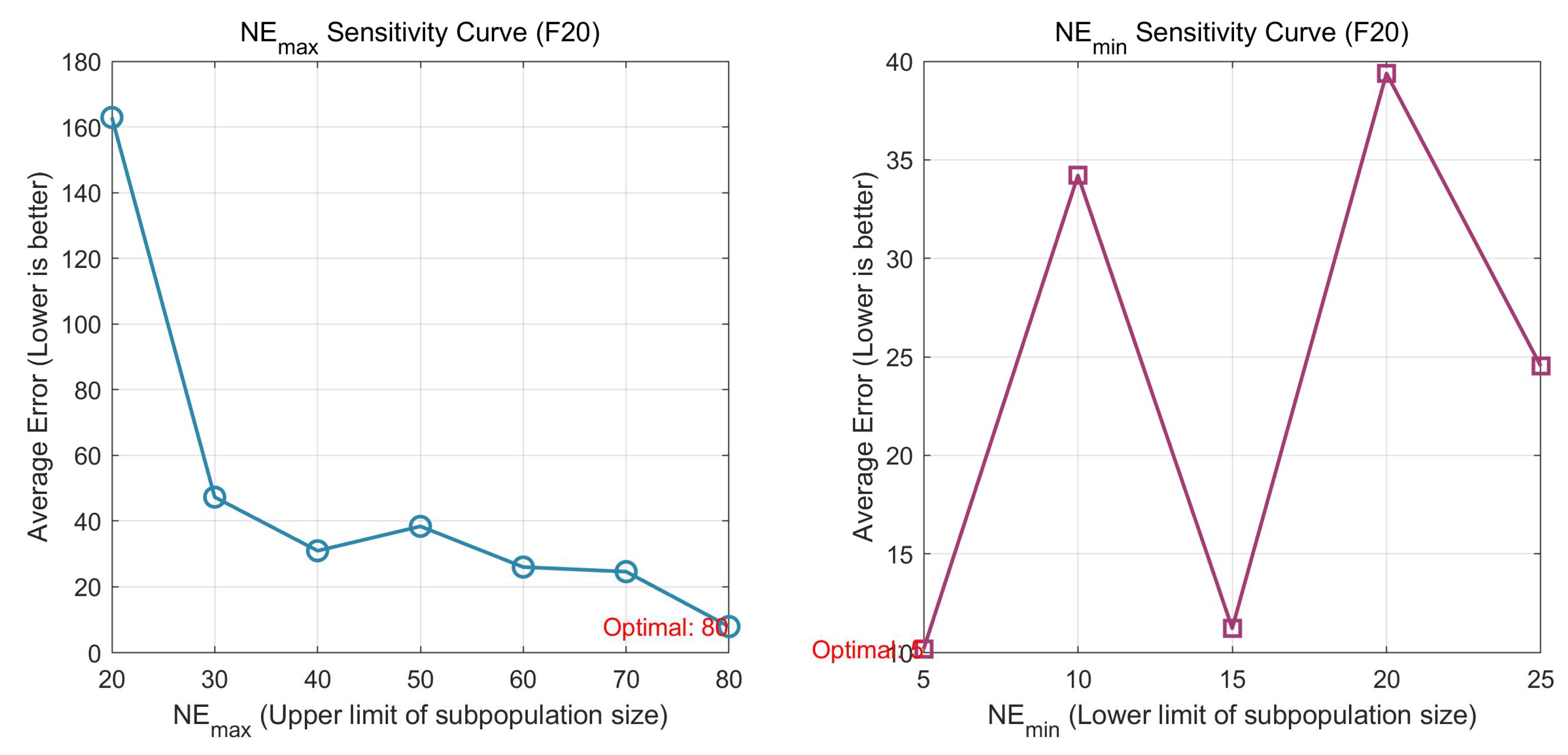
The size of the subpopulations should be controlled within a reasonable range to prevent extreme population structures. In this paper, appropriate constraints are imposed on the sizes of the subpopulations of the Differential Evolution (DE) and Particle Swarm Optimization (PSO) algorithms. Specifically, the upper limit NE_max and lower limit NE_min of the subpopulation size are set to 40 and 10, respectively. The sizes of the PSO and DE subpopulations in the next generation are determined by Equations (16) and (17), respectively:

$$N{E}_{\mathrm{PSO}}^{t+1}=\left\{\begin{array}{c}N{E}_{\max }N{E}_{\mathrm{PSO}}^t+p_{\mathrm{PSO}}^{t+1}\cdot N{E}_{\mathrm{PSO}}^{t }>N{E}_{\max }\hfill \\ N{E}_{\min }N{E}_{\mathrm{PSO}}^t+p_{\mathrm{PSO}}^{t+1}\cdot N{E}_{\mathrm{PSO}}^{t }<N{E}_{\min }\hfill \\ N{E}_{\mathrm{PSO}}^{t }+p_{\mathrm{PSO}}^{t+1}\cdot N{E}_{\mathrm{PSO}}^{t }\mathrm{otherwise}\hfill \end{array}\right.$$

(16)

$$N{E}_{\mathrm{DE}}^{\mathrm{t}+1}=\left\{\begin{array}{c}N{E}_{\max }N{E}_{\mathrm{DE}}^{\mathrm{t} }+p_{\mathrm{DE}}^{\mathrm{t}+1}\cdot N{E}_{\mathrm{DE}}^{\mathrm{t} }>N{E}_{\max }\hfill \\ N{E}_{\min }N{E}_{\mathrm{DE}}^{\mathrm{t}}+p_{\mathrm{DE}}^{\mathrm{t}+1}\cdot N{E}_{\mathrm{DE}}^{\mathrm{t} }<N{E}_{\min }\hfill \\ N{E}_{\mathrm{DE}}^{\mathrm{t}}+p_{\mathrm{DE}}^{\mathrm{t}+1}\cdot N{E}_{\mathrm{DE}}^{\mathrm{t} }\mathrm{otherwise}\hfill \end{array}\right.$$

(17)

where $N{E}_{\mathrm{PSO}}^{t+1}$ is the scale of the PSO elite particles to be updated in the (t + 1)-th generation, $N{E}_{\mathrm{PSO}}^t$ is the scale of the PSO elite particles in the t-th generation, $p_{\mathrm{PSO}}^{t+1}$ is the update ratio of the PSO elite particles in the (t + 1)-th generation, $N{E}_{\mathrm{DE}}^{t+1}$ is the scale of the DE elite particles to be updated in the (t + 1)-th generation, $N{E}_{\mathrm{DE}}^t$ is the scale of the DE elite particles in the t-th generation, $p_{\mathrm{DE}}^{t+1}$ is the update ratio of the DE elite particles in the (t + 1)-th generation, and NE_max and NE_min are the upper and lower limits of the subpopulation scale, respectively. The operation of the DE/PSO elite particle scale in the (t + 1)-th generation is as shown in Algorithm 2.

Algorithm 2 Module 2: Elite Population Size Adjustment based on Hooke’s Law

Require: $p_{DE}^t$, $p_{PSO}^t$, $N{E}_{DE}^t$, $N{E}_{PSO}^t$, NEmax = 40, NEmin = 10, NP, ND

Ensure: $N{E}_{DE}^{t+1}$, $N{E}_{PSO}^{t+1}$

1:   calculate $p_{DE}^{t+1}$ and $p_{PSO}^{t+1}$

2:   $p_{DE}^{t+1}=(outpu{t}_{\max }-outpu{t}_{\min })({\displaystyle \frac{p_{DE}^t}{inpu{t}_{\max }-inpu{t}_{\min }}}-{\displaystyle \frac{inpu{t}_{\max }+inpu{t}_{\min }}{2(inpu{t}_{\max }-inpu{t}_{\min })}})$

3:   $p_{PSO}^{t+1}=(outpu{t}_{\max }-outpu{t}_{\min })({\displaystyle \frac{p_{PSO}^t}{inpu{t}_{\max }-inpu{t}_{\min }}}-{\displaystyle \frac{inpu{t}_{\max }+inpu{t}_{\min }}{2(inpu{t}_{\max }-inpu{t}_{\min })}})$

4:   $N{E}_{\mathrm{DE}}^{\mathrm{t}+1}=N{E}_{\mathrm{DE}}^{\mathrm{t}}+p_{\mathrm{DE}}^{\mathrm{t}+1}\cdot N{E}_{\mathrm{DE}}^{\mathrm{t}}$

5:   $N{E}_{DE}^{t+1}$= max(NEmin, min(NEmax, $N{E}_{DE}^{t+1}$))

6:   $N{E}_{PSO}^{t+1}=N{E}_{PSO}^{t }+p_{PSO}^{t+1}\cdot N{E}_{PSO}^t$

7:   $N{E}_{PSO}^{t+1}$= max(NEmin, min(NEmax, $N{E}_{PSO}^{t+1}$))

return $N{E}_{DE}^{t+1}$, $N{E}_{PSO}^{t+1}$

3.2. Adaptive Acceleration Coefficient Strategy Based on Gaussian Guidance and Empirical Traceability

From Equation (1), it can be seen that c₁ and c₂ are acceleration coefficients, where c₁ represents the degree to which a particle is influenced by its own experience, and c₂ represents the degree to which a particle is influenced by the group’s experience. Iteration requires early exploration ability and later exploitation ability. Therefore, in the early stage of iteration, a larger c₁ and a smaller c₂ should be set to enhance the diversity of the population. Conversely, in the later stage of evolution, a smaller c₁ and a larger c₂ should be adopted to accelerate the convergence speed of the algorithm. Thus, both c₁ and c₂ are linearly adjusted during the optimization process, with c₁ increasing linearly and c₂ decreasing linearly.

However, regular c₁ and c₂ may lead to the neglect of some new areas. This paper adopts the “concentration” principle in line with the Gaussian distribution to ensure that the Particle Swarm Optimization (PSO) algorithm can effectively search based on reasonable experience in most cases, thereby avoiding confusion in the search process; the “long tail” property of the Gaussian distribution ensures that PSO explores new areas with a small probability, avoiding premature convergence. Therefore, in HLCM-DHPSO, the definitions of c₁ and c₂ are respectively given by Equations (18) and (19):

$$c_1=randn((c_{1,ini}-{\displaystyle \frac{iter}{ite{r}_{\max }}}(c_{1,ini}-c_{1,final})),0.1)$$

(18)

$$c_2=randn((c_{2,ini}-{\displaystyle \frac{iter}{ite{r}_{\max }}}(c_{2,ini}-c_{2,final})),0.1)$$

(19)

where iter and iter_max represent the current iteration number and the maximum number of iterations, respectively. c_1,init and c_1,final are the initial and final values of c₁, while c_2,init and c_2,final are the initial and final values of c₂. Ratnaweera et al. [15] suggested that the value of c₁ should linearly decrease from 2.5 to 0.5, while c₂ should linearly increase from 0.5 to 2.5.

In the later stage of the algorithm’s evolution, the lack of particle diversity may lead to a slowdown in the evolution speed and getting stuck in a local optimum. At this point, appropriately adjusting the acceleration coefficients c₁ and c₂ can help the algorithm escape from the local optimum. During the evolution process, the c₁ and c₂ values that are beneficial to the algorithm’s improvement are saved in the recordC file. The calculation Equations for the c₁ and c₂ files that are beneficial to the algorithm’s improvement are given by (20) and (21):

$$record{c}_1^{\mathrm{j}+1}=c_1^{\mathrm{j}+1}f(x_{\mathrm{i}}^{\mathrm{t}+1})<f(x_{\mathrm{i}}^{\mathrm{t}})$$

(20)

$$record{c}_2^{\mathrm{j}+1}=c_2^{\mathrm{j}+1}f(x_{\mathrm{i}}^{\mathrm{t}+1})<f(x_{\mathrm{i}}^{\mathrm{t}})$$

(21)

where ${recordc}_1^{j+1}$ and ${recordc}_2^{j+1}$ are the acceleration coefficients c₁ and c₂ of the (j + 1)-th archived entry, and f($x_i^t$) is the fitness value of the i-th particle in the t-th generation.

The recordc archive stores the c₁ and c₂ that are beneficial to the algorithm improvement, with a maximum storage capacity of RN. The recordc archive is shown in

Table 1. Acceleration coefficient c₁, c₂ in archive recordc.

Index	1	2	……	RN − 1	RN
c1	$c_1^1$	$c_1^2$		$c_1^{RN-1}$	$c_1^{RN}$
c2	$c_2^1$	$c_2^2$		$c_2^{RN-1}$	$c_2^{RN}$

.

When the number of c₁ and c₂ in the archive exceeds the limit, the records with poorer performance are eliminated based on the algorithm improvement rate. The algorithm improvement rate is as shown in Equation (22) and the acceleration coefficient at the position with the smallest r_k in recordc is eliminated:

$$r_{\mathrm{k}}={\displaystyle \frac{f(x_{\mathrm{k}})-f(x_{\mathrm{k}-1})}{{\displaystyle {\sum }_{\mathrm{k}=1}^{\mathrm{RN}}(f(x_{\mathrm{k}})-f(x_{\mathrm{k}-1}))}}}$$

(22)

where $r_k$ is the improvement rate of the k-th record in the acceleration coefficient archive to the algorithm, and RN is the archive size.

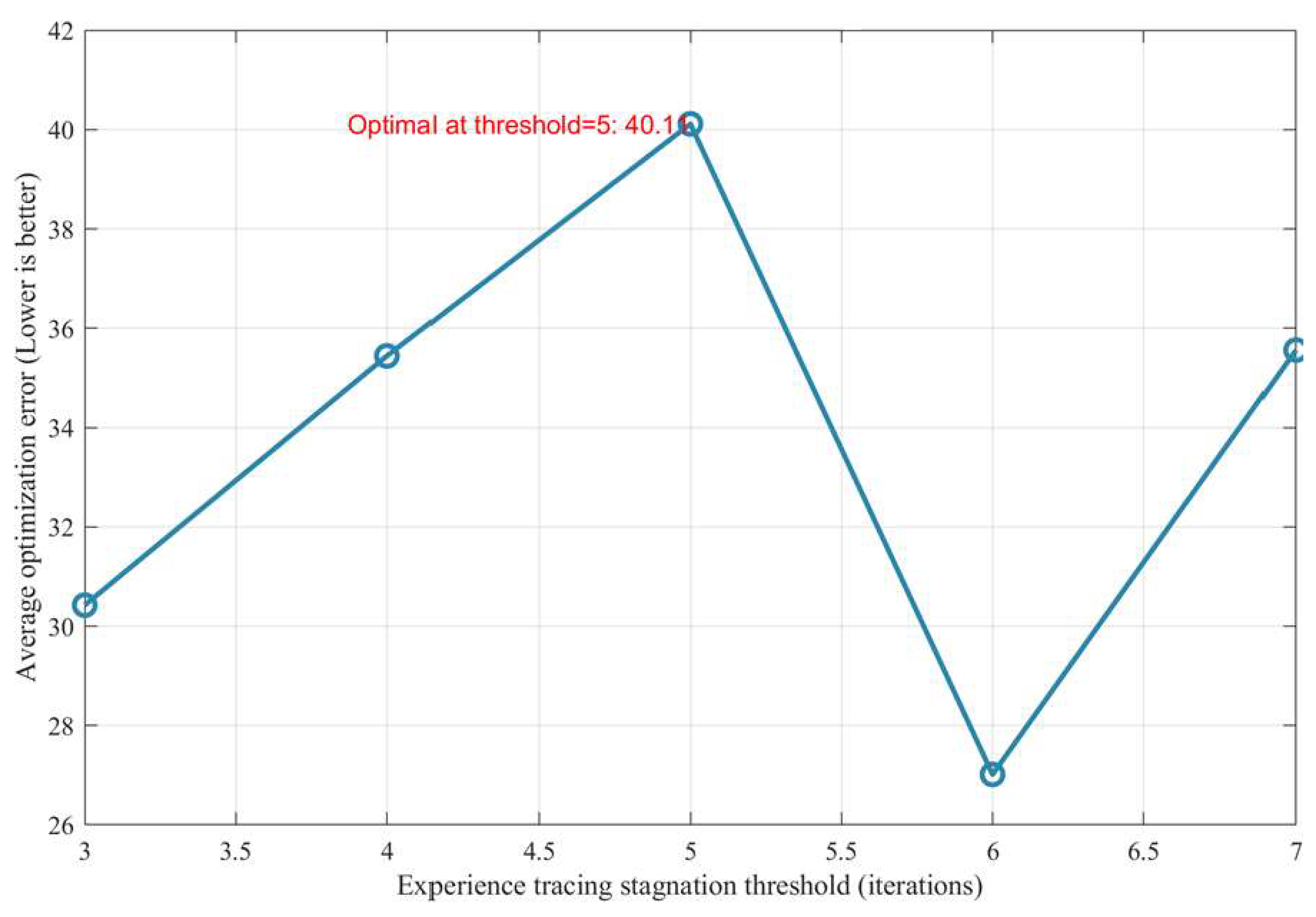
If the fitness does not improve in six consecutive iterations of the algorithm, the algorithm will trace back to the historical successful experience. From the perspective of stability, the algorithm traces back to the average of the previous experience. However, if only the historical experience is relied on for average calculation, the ordinary performance and excellent performance experiences will be treated equally, which may cause c₁ and c₂ to shift towards undesirable data, thereby reducing the search performance. To enhance the robustness of the algorithm, this study introduces a method for adaptively tracing back the acceleration coefficients c₁ and c₂ based on the algorithm’s improvement rate. The new acceleration coefficients meanc₁ and meanc₂ are updated according to Equations (23) and (24):

$$mean{c}_1={\displaystyle \frac{1}{RN}}{\displaystyle \sum _{k=1}^{RN}{r}_k}\cdot c_1^k$$

(23)

$$mean{c}_2={\displaystyle \frac{1}{RN}}{\displaystyle \sum _{k=1}^{RN}{r}_k}\cdot c_2^k$$

(24)

where $r_k$ represents the improvement rate, which is given by Equation (22). RN is the number of records in recordc, $c_1^k$ is the first acceleration coefficient c₁ of the k-th record in recordc, and $c_2^k$ is the second acceleration coefficient c₂ of the k-th record in recordc. The operations of acceleration coefficients c₁ and c₂ are as shown in Algorithm 3.

Algorithm 3 Module 3: Acceleration Coefficients Update

Require: iter, itermax, recordC, fcurr, fprev, stagnation, RN = 20

Ensure: $c_1^t$, $c_2^t$

1:   $c_1=randn((c_{1,ini}-{\displaystyle \frac{iter}{ite{r}_{\max }}}(c_{1,ini}-c_{1,final})),0.1)$                   (18)

2:   $c_2=randn((c_{2,ini}-{\displaystyle \frac{iter}{ite{r}_{\max }}}(c_{2,ini}-c_{2,final})),0.1)$                   (19)

3:   if fcurr < fprev  then

4:             $record{c}_1^{j+1}=c_1^{j+1}f(x_i^{t+1})<f(x_i^t)$                                 (20)

5:             $record{c}_2^{j+1}=c_2^{j+1}f(x_i^{t+1})<f(x_i^t)$                                 (21)

6:             $r_k={\displaystyle \frac{f(x_k)-f(x_{k-1})}{{\displaystyle {\sum }_{k=1}^{RN}(f(x_k)-f(x_{k-1}))}}}$                                      (22)

7:             $\mathrm{Add} [c_1^{j+1}$$, c_2^{j+1}$] to recordC; trim to RN if oversized based on $r_k^t$

8:   end if

9:   if stagnation ≥ 6 and recordC ≠ Ø then

10:            $mean{c}_1={\displaystyle \frac{1}{RN}}{\displaystyle \sum _{k=1}^{RN}{r}_k}\cdot c_1^k$                                            (23)

11:           $mean{c}_2={\displaystyle \frac{1}{RN}}{\displaystyle \sum _{k=1}^{RN}{r}_k}\cdot c_2^k$                                             (24)

12:            $c_1^t$ $={\mathit{meanc}}_1; c_2^t$ = meanc2

13: end if

14: $c_1^t$ $= \max (0.5, \min (2.5, c_1^t$$\left)\right); c_2^t$ $=\max (0.5, \min (2.5, c_2^t$))

return $c_1^t$$, c_2^t$

3.3. Sine-Improved and Experience Tracing-Based Adaptive Inertia Weight Strategy

During the iterative process, a larger inertia weight ω is conducive to a thorough overall exploration of the global solution space, while a smaller inertia weight ω is more beneficial for local fine exploitation. Therefore, in this paper, a linearly decreasing inertia weight strategy is adopted during the evolutionary process, and inspired by the Sine function, the Sine function is introduced to perturb the inertia weight to enhance the dynamic adjustment ability of the search process. The specific expression of the inertia weight ω is shown in Equation (25):

$$\left\{\begin{array}{c}{\omega }^{iter}={\omega }_i-{\displaystyle \frac{iter}{ite{r}_{\max }}}({\omega }_i-{\omega }_f){\displaystyle \frac{iter}{ite{r}_{\max }}}\le 0.5 \hfill \\ {\omega }^{iter}=({\omega }_i-{\displaystyle \frac{iter}{ite{r}_{\max }}}({\omega }_i-{\omega }_f))\cdot \sin (0\sim pi){\displaystyle \frac{iter}{ite{r}_{\max }}}>0.5\hfill \end{array}\right.$$

(25)

where ω_i and ω_f represent the initial and maximum values of ω respectively, iter is the current iteration number, and iter_max is the maximum iteration number. ω_i is set to 0.9 and ω_f is set to 0.4.

The Sine function perturbation is applied when iter/iter_max > 0.5. Specifically, the input of the Sine function is randomly sampled from the interval [0, π] using a uniform distribution (i.e., rand () × π, where rand () generates a random float in [0, 1]). This ensures a moderate and unbiased perturbation intensity to the inertia weight.

In the later stage of algorithm evolution, the lack of particle diversity may lead to a slowdown in the evolution speed and getting trapped in local optimal solutions. At this point, by appropriately adjusting the inertia weight ω, the algorithm can be promoted to escape from local optima. During the evolution process, the ω that is beneficial to the algorithm improvement is saved to the recordω archive, and the calculation equation of the ω archive that is beneficial to the algorithm improvement is given by Equation (26):

$$rcord{\omega }^{j+1}={\omega }^{i+1},(f(x_i^{t+1})<f(x_i^t))$$

(26)

where $rcord{\omega }^{j+1}$ is the acceleration coefficient ω of the (j + 1)-th entry in the archive, and f($x_i^t$) is the fitness value of the i-th particle in the t-th generation.

The recordω archive stores the inertia weights that are beneficial to the algorithm improvement, with a maximum storage capacity of RN. The recordω archive is shown in

Table 2. Inertia weight ω archive recordω.

Index	1	2	……	RN − 1	RN
ω1	ω1	ω2	……	ωRN−1	ωRN

.

When the number of ω in the archive exceeds the limit, the records with poorer performance are eliminated based on the algorithm improvement rate. The algorithm improvement rate is as shown in Equation (22), and the ω with the smallest $r_k$ in recordω is eliminated.

Similarly to the acceleration coefficient, if the fitness does not improve in six consecutive iterations, the algorithm will trace back to the historical successful experience. Considering the stability, the algorithm traces back to the mean of the previous experience. However, if only the historical experience is averaged, the ordinary and excellent experiences will be treated equally, which may cause ω to shift towards undesirable data and thus reduce the search performance. To enhance the robustness of the algorithm, this study introduces a method for adaptively tracing back the inertia weight ω based on the algorithm improvement rate. The new inertia weight meanω is updated according to Equation (27).

$$\left\{\begin{array}{c}mean\omega ={\displaystyle \frac{1}{RN}}{\displaystyle \sum _{k=1}^{RN}{r}_k\cdot {\omega }^k}\hfill \\ {\omega }^t=mean\omega \hfill \end{array}\right.$$

(27)

From Equation (11), it can be seen that HLCM-DHPSO integrates the advantages of differential algorithm and particle swarm optimization algorithm in the optimization process, effectively balancing the diversity of particles and the convergence speed. The velocity update equation of the i-th particle is shown in Equation (28). The position update equation of the particle is given by Equation (2):

$$v_{i,j}^{t+1}=\left\{\begin{array}{c}{\omega }^t\cdot v_{i,j}^t+c_1^t\cdot r_1\cdot (e{x}_{i,j}^t-x_{i,j}^t)+c_2^t\cdot r_2\cdot (Q_{i,j}^t-x_{i,j}^t)x_i^t\notin P{R}^t \hfill \\ {\omega }^t\cdot v_{i,j}^t+c_1^t\cdot r_1\cdot (e{x}_{i,j}^t-x_{i,j}^t)+c_2^t\cdot r_2\cdot (p{b}_{i,j}-x_{i,j}^t) \mathrm{otherwise}\hfill \end{array}\right.$$

(28)

where $v_{i,j}^{t+1}$ represents the velocity of the i-th particle in the j-th dimension at the (t + 1)-th generation. $x_{i,j}^{t+1}$ represents the position of the i-th particle in the j-th dimension at the (t + 1)-th generation. i = {1, 2, 3, …, NP}, where NP is the size of the particle population. ω is the inertia weight, given by Equations (25)–(27), c₁ and c₂ are the acceleration coefficients, given by Equations (18)–(24). r₁ and r₂ are two random numbers distributed between [0, 1], $e{x}_{i,j}^t$ is given by Equation (12), $p{b}_{i,j}^t$ represents the value of the j-th dimension of the individual optimal position of the ith particle in the t-th generation. $Q_{i,j}^t$ is given by Equation (13). $P{R}^t$ is given by Equation (5).

To sum up, the details of the dual-population hybrid particle swarm optimization algorithm based on Hooke’s law competition mechanism, HLCM-DHPSO, are shown in Algorithm 4.

Algorithm 4 Main Algorithm: HLCM-DHPSO

Require: NP = 50, ND = 50, D = 30, tmax = 1000, F = 0.5, CR = 0.5, NP = 100

Ensure: gbest, fgbest

1:   Randomly initialize position vectors XPSO, XDE and velocity vectors v

2:   Calculate fitness f(XPSO) and f(XDE) for all individuals

3:   gbest = min([f(XPSO); f(XDE)])

4:   NEPSO = ⌊NP/2⌋, NEDE = ⌊ND/2⌋

5:   DPR = Top fPSO/DE of XPSO/DE based on Equations (4)–(6)

6:   recordC = Ø; stagnation = 0

7:   for t = 1 to tmax do

8:           Calculate the value of inertia weight ωᵗ base on Equations (25)–(27)

9:           for i = 1 to NP do

10:                 $f_{prev}=f_i^{t-1};f_{curr}=f_i^t$

11:                stagnation = |fcurr − fprev| < 10−8 ? stagnation + 1: 0

12:                $[c_1^t$$,c_2^t$] = MODULE3(t, tmax, recordC, fcurr, fprev, stagnation, RN)

13:          end for

14:          $p_{\mathrm{PSO}/\mathrm{DE}}^{t-1}={\displaystyle \frac{\mathrm{size}(P{R}^{t-1}/E{R}^{t-1})}{\mathrm{size}(DP{R}^{t-1})}}$

15:          $[N{E}_{\mathrm{DE}}^t$$, N{E}_{\mathrm{PSO}}^t$$]=\mathrm{MODULE}2(p_{\mathrm{PSO}}^{t-1}$$, p_{\mathrm{DE}}^{t-1}$$, N{E}_{\mathrm{DE}}^{t-1}$$, N{E}_{\mathrm{PSO}}^{t-1}$, 40, 10, NP, ND)

16:          $DP{R}^t$$=\mathrm{Top} N{E}_{\mathrm{PSO}/\mathrm{DE}}^t$$\mathrm{of} N{E}_{\mathrm{PSO}/\mathrm{DE}}^{t-1}$

17:          $[e{x}_{i,j}^t$$, Q^k, x_{\mathrm{DE}}^t$$]=\mathrm{MODULE}1(X_{\mathrm{PSO}}^{t-1}$$, X_{\mathrm{DE}}^{t-1}$, F, CR, D, LB, UB, t, tmax)

18:          for i = 1 to NP do

19:                 $\mathrm{Update} v_i^t$ $\mathrm{and} x_i^t$ based on Equation (28) and Equation (2), respectively;

20:                 $\mathrm{Update} pbes{t}_{\mathrm{PSO}}^t$

21:                 Update gbest

22:          end for

24: end for

return gbest, fgbest

3.4. Theoretical Analysis of HLCM-DHPSO

To justify the rationality of Hooke’s Law Competition Mechanism and the overall algorithm, this section provides a concise theoretical analysis focusing on convergence, stability, and its quantitative impact on exploration-exploitation balance, all based on the core velocity updated equation, Equation (28)

3.4.1. Convergence Analysis

The convergence of HLCM-DHPSO is guaranteed by two key properties derived from Equation (28).

(1)

Boundedness of Velocity and Position

For both elite particles ($x_i^t$ ∈ $Q_{i,j}^t$) and ordinary particles (otherwise) in Equation (28). Inertia weight ω^t ∈ [0.4, 0.9] (Section 3.3), acceleration coefficients $c_1^{\mathrm{t}}$, $c_2^{\mathrm{t}}$ ∈ [0.5, 2.5] (Section 3.2), ensuring the weight of each update term is bounded.

Reference positions ($e{x}_{i,j}^t$, $p{b}_{i,j}^t$, $Q_{i,j}^t$) are all within the search space [LB, UB], so the position differences ($e{x}_{i,j}^t-x_{i,j}^t$, etc.) are bounded by [LB, UB]. Thus, $v_{i,j}^t$ is bounded by v_max = 0.2 × (UB − LB) and $x_{i,j}^{t+1}=x_{i,j}^t+v_{i,j}^{t+1}$ remains within the search space.

(2)

Monotonic Improvement of Fitness

In each iteration, pbest and gbest are only updated when a better fitness value is obtained, so the global fitness sequence $f(gbes{t}^t)$ is non-increasing. By the Monotone Bounded Theorem, $f(gbes{t}^t)$ converges to a limit value. Combined with the DE subpopulation’s global exploration (Section 3.1) and Sine perturbation of inertia weight (Section 3.3), the algorithm can escape local optima with non-zero probability, ensuring convergence to the global optimum.

3.4.2. Stability of Hooke’s Law Competition Mechanism

The HLCM-DHPSO maintains stable co-evolution of dual populations through two constraints

(1) Bounded Adjustment Ratio: The elite population size (NE_PSO, NE_DE) is adjusted within ±10% (Equations (16) and (17)), avoiding extreme sizes (e.g., NE_DE < 10 or NE_PSO > 40) that would disrupt exploration-exploitation balance.

(2) When the PSO and DE subpopulations perform equally well (σ ∈ [0, 1], Section 3.1), the adjustment ratio ε = k_Hooke (σ − 0.5) = 0, meaning no adjustment is made. This equilibrium point prevents continuous oscillation of subpopulation sizes, ensuring stable co-evolution.

3.4.3. Quantitative Impact on Exploration-Exploitation Balance

The HLCM-DHPSO quantitatively regulates the balance by adjusting the elite population size, which directly correlates with exploration/exploitation intensity.

Let $p_{\mathrm{PSO}}^1=N{E}_{\mathrm{PSO}}^1/(N{E}_{\mathrm{PSO}}^1+N{E}_{\mathrm{DE}}^1)$ (proportion of PSO elite particles) and $p_{\mathrm{DE}}^1=1-p_{\mathrm{PSO}}^1$ (proportion of DE elite particles). Since PSO excels at exploitation, exploitation intensity is positively correlated with P_PSO, and Since DE excels at exploration, exploration intensity is positively correlated with P_DE.

The HLCM-DHPSO adjusts $p_{\mathrm{DE}}^{t+1}$ and $p_{\mathrm{PSO}}^{t+1}$ based on Equations based on Equations (14) and (15). If there is any change in the performance of PSO, $N{E}_{\mathrm{PSO}}^{t+1}$ and $N{E}_{\mathrm{DE}}^{t+1}$ are updated by Equation (16) and (17) and vice versa. This quantitative adjustment ensures a dynamic balance between exploration and exploitation.

3.4.4. Computational Complexity Analysis

The computational complexity of HLCM-DHPSO is analyzed per iteration and compared with representative comparison algorithms (GGL-PSOD, SWFA, CRADE) to quantify its theoretical overhead. Let D be the problem dimension, N_total be the total population size (N_PSO + N_DE), and RN be the capacity of the experience-tracing archive (20 in this work).

(1) Per-iteration complexity of HLCM-DHPSO

The core operations include: (1) velocity and position update (Equation (28)) for dual populations: O (N_total∙D); (2) Hooke’s Law competition mechanism (elite size adjustment): O (N_elite) (negligible compared to N_total∙D); (3) experience-tracing for parameters: O (RN) (constant time). Thus, the total per-iteration complexity of HLCM-DHPSO is O (N_total∙D), which is the same asymptotic order as standard PSO, DE, and hybrid variants.

(2) Time Complexity Comparison of HLCM-DHPSO and Competitive Algorithms

The core complexity of the HLCM-DHPSO algorithm is O (N_total∙D), and its additional overhead is a constant O (RN + N_elite). The core complexity of the GGL-PSOD algorithm is O (N∙D), and its additional overhead is O (N) for ring topology update. The core complexity of the SWFA algorithm is O (N∙D), and its additional overhead is negligible due to the lightweight sliding window. The core complexity of the CRADE algorithm is O (N∙D), and its additional overhead is O (N∙D) for differential mutation of all individuals. It is proven that compared with its competitors, HLCM-DHPSO does not introduce an increased asymptotic complexity, and its additional cost is limited to constant-time auxiliary modules.

4. Experimental Verification and Comparison

4.1. Experimental Setup

To explore the characteristics of HLCM-DHPSO and verify its performance, a series of experiments were conducted in this section. These experiments verified the characteristics of the proposed strategies of HLCM-DHPSO. In this study, eight other algorithms were selected as comparison algorithms. Four advanced Particle Swarm Optimization (PSO) variants were GGL-PSOD [18], Spade-PSO [35], DPSO-PI [17], and CPSO [36], and four other advanced algorithms were CRADE [37], SWFA [38], HHO [39], and WOA [40]. The parameter settings are summarized in

Table 3. Parameter Settings of Comparative Algorithms.

Algorithms	Year	Parameter Settings
HLCM-DHPSO	2026	ω ∈ [0.9, 0.4], p, c1, and c2 are adjustable, K = 2
GGL-PSOD	2019	ω ∈ [0.9, 0.4], c1 ∈ [2.5, 0.5], c2 ∈ [0.5, 2.5], Pm = 0.01, Sg = 7
Spade-PSO	2023	ω ∈ [0.99∼0.2], c1 ∈ [2.5, 0.5], c2 ∈ [0.5, 2.5], c ∈ [3, 1.5], k0 = 2, vk = 6
DPSO-PI	2023	ω ∈ [0.8∼0.3], p ∈ [0.62∼0.2], k ∈ [2∼100]
CPSO	2004	c1 = c2 = 1.49, f0 = 100, f1 = 0.02, f2 = 5.00, f3 = 100, f4 = 0.1
CRADE	2023	k1 ∈ [0, 1], k2 ∈ [0, 1], k1 + k2 = 1, σ = 0.1, H = 1
SWFA	2022	α = 0.5, β0 = 1, γ = 1/(ub − lb)2, offset = 5
HHO	2019	β = 1.5, E0 ∈ [−1, 1], J = 2(1 − rand())
WOA	2016	a ∈ [2, 0], b = 1, C ∈ [0, 2], p = 0.5, r ∈ [0, 1]

, which are the same as those in the corresponding literature.

All algorithms were implemented in MATLAB 2020b and run on a personal computer (manufactured by HP Inc., Palo Alto, CA, USA; assembled in Chongqing, China) equipped with an Intel Core i7-6700HQ CPU (2.6 GHz, 4 cores, 8 threads)and 16 GB of memory. The CPU was sourced from Intel Corporation, Santa Clara, CA, USA.

4.2. Algorithm Performance Comparison and Analysis

To fully evaluate the performance of HLCM-DHPSO and ensure the fairness of the experiment, 30 identical benchmark functions from the CEC2017 benchmark function set are used. This benchmark function suite includes four types of test functions: 3 unimodal functions (F₁–F₃), 7 simple multimodal functions (F₄–F₁₀), 10 hybrid functions (F₁₁–F₂₀), and 10 composite functions (F₂₁–F₃₀). All algorithms are evaluated on the CEC2017 benchmark function set (dimension D = 30), with a population size of NP = 100 for each algorithm. The maximum number of function evaluations is set to MaxFE = 10,000 × D.

The four different types of functions are independently run 51 times using algorithm HLCM-DHPSO and four PSO variants (GGL-PSOD, SPADE-PSO, DPSO-PI, and CPSO). The average value (Mean) of the 51 runs is taken.

Table 4. Comparison Experiment Results of PSO Variants and HLCM-DHPSO on F₁–F₃.

NO.	Criteria	CPSO	DPSO-PI	SPADE-PSO	GGL-PSOD	HLCM-DHPSO
F1	mean	2.21E + 10 (+)	2.70E + 03 (+)	3.62E + 03 (+)	3.29E + 03 (+)	2.95E − 02
	std	8.31E + 09	3.14E + 03	4.24E + 03	4.24E + 03	1.49E + 02
F2	mean	3.00E + 40 (+)	1.16E + 05 (−)	3.82E + 04 (−)	9.31E + 01 (−)	1.42E + 13
	std	1.67E + 41	8.07E + 05	2.55E + 05	2.79E + 02	9.07E + 13
F3	mean	8.46E + 04 (+)	3.41E − 01 (−)	3.77E − 01 (−)	8.51E − 09 (−)	1.62E + 02
	std	4.64E + 04	1.06E + 00	1.10E + 00	2.44E − 08	1.97E + 02

,

Table 5. Comparison Experiment Results of PSO Variants and HLCM-DHPSO on F₄–F₁₀.

NO.	Criteria	CPSO	DPSO-PI	SPADE-PSO	GGL-PSOD	HLCM-DHPSO
F4	mean	2.41E + 03 (+)	8.27E + 01 (+)	5.98E + 01 (−)	6.14E + 01 (−)	6.41E + 01
	std	1.61E + 03	2.10E + 01	1.77E + 01	6.55E + 00	2.72E + 01
F5	mean	1.85E + 02 (+)	4.33E + 01 (+)	3.90E + 01 (+)	2.90E + 01 (−)	3.10E + 01
	std	3.61E + 01	1.32E + 01	1.08E + 01	7.71E + 00	9.98E + 00
F6	mean	3.08E + 01 (+)	1.63E − 08 (−)	3.08E − 08 (−)	1.51E − 07 (−)	3.00E − 03
	std	9.93E + 00	8.13E − 08	1.60E − 07	6.84E − 07	1.48E − 02
F7	mean	3.81E + 02 (+)	8.27E + 01 (+)	8.16E + 01 (+)	6.61E + 01 (≈)	6.61E + 01
	std	1.50E + 02	1.56E + 01	1.64E + 01	1.04E + 01	1.75E + 01
F8	mean	1.87E + 02 (+)	4.44E + 01 (+)	4.34E + 01 (+)	3.22E + 01 (+)	2.91E + 01
	std	3.93E + 01	1.24E + 01	1.18E + 01	1.05E + 01	7.91E + 00
F9	mean	6.12E + 03 (+)	2.52E + 00 (+)	2.51E + 00 (+)	9.42E − 02 (+)	0.00E + 00
	std	2.37E + 03	5.72E + 00	5.32E + 00	2.22E − 01	0.00E + 00
F10	mean	4.53E + 03 (+)	2.44E + 03 (+)	2.36E + 03 (+)	2.16E + 03 (−)	2.20E + 03
	std	7.01E + 02	3.95E + 02	4.98E + 02	5.79E + 02	7.42E + 02

,

Table 6. Comparison Experiment Results of PSO Variants and HLCM-DHPSO on F₁₁–F₂₀.

NO.	Criteria	CPSO	DPSO-PI	SPADE-PSO	GGL-PSOD	HLCM-DHPSO
F11	mean	2.72E + 03 (+)	5.44E + 01 (+)	5.18E + 01 (+)	4.43E + 01 (+)	1.54 E + 01
	std	4.85E + 03	2.82E + 01	2.57E + 01	3.05E + 01	1.70E + 01
F12	mean	1.26E + 09 (+)	2.96E + 04 (+)	2.92E + 04 (+)	2.08E + 04 (+)	9.18E + 03
	std	1.17E + 09	1.46E + 04	1.50E + 04	9.79E + 03	6.01E + 03
F13	mean	6.29E + 08 (+)	8.60E + 03 (+)	9.40E + 03 (+)	1.17E + 04 (+)	6.36E + 01
	std	1.01E + 09	8.19E + 03	7.85E + 03	1.23E + 04	2.35E + 01
F14	mean	7.01E + 05 (+)	4.87E + 03 (+)	3.47E + 03 (+)	2.81E + 03 (+)	2.66E + 01
	std	1.95E + 06	5.00E + 03	3.61E + 03	2.73E + 03	9.95E + 00
F15	mean	3.56E + 07 (+)	9.49E + 02 (+)	7.83E + 02 (+)	2.97E + 03 (+)	9.39E + 00
	std	1.77E + 08	1.01E + 03	6.73E + 02	4.10E + 03	2.62E + 00
F16	mean	1.75E + 03 (+)	4.99E + 02 (+)	4.31E + 02 (+)	3.58E + 02 (+)	5.95E + 01
	std	5.09E + 02	2.18E + 02	1.63E + 02	2.04E + 02	1.71E + 02
F17	mean	7.89E + 02 (+)	7.89E + 01 (+)	8.94E + 01 (+)	5.13E + 01 (+)	4.59E + 01
	std	2.48E + 02	4.70E + 01	5.00E + 01	3.93E + 01	2.85E + 01
F18	mean	4.76E + 06 (+)	1.11E + 05 (+)	1.25E + 05 (+)	7.39E + 04 (+)	1.68E + 04
	std	1.70E + 07	7.89E + 04	9.23E + 04	5.26E + 04	1.17E + 04
F19	mean	8.58E + 07 (+)	6.55E + 02 (+)	7.57E + 02 (+)	4.03E + 03 (+)	8.56E + 00
	std	2.00E + 08	6.84E + 02	7.56E + 02	5.48E + 03	2.88E + 00
F20	mean	5.46E + 02 (+)	1.44E + 02 (+)	1.41E + 02 (+)	1.09E + 02 (+)	6.13E + 00
	std	1.81E + 02	7.80E + 01	6.61E + 01	7.63E + 01	6.35E + 01

and

Table 7. Comparison Experiment Results of PSO Variants and HLCM-DHPSO on F₂₁–F₃₀.

NO.	Criteria	CPSO	DPSO-PI	SPADE-PSO	GGL-PSOD	HLCM-DHPSO
F21	mean	3.93E + 02 (+)	2.39E + 02 (+)	2.33E + 02 (+)	2.33E + 02 (+)	2.32E + 02
	std	3.82E + 01	2.80E + 01	3.41E + 01	9.77E + 00	8.06E + 00
F22	mean	4.43E + 03 (+)	1.00E + 02 (≈)	1.00E + 02 (≈)	1.00E + 02 (≈)	1.00E + 02
	std	1.09E + 03	7.40E − 01	4.82E − 01	4.82E − 01	1.41E − 13
F23	mean	6.36E + 02 (+)	3.96E + 02 (+)	3.92E + 02 (+)	3.79E + 02 (+)	3.78E + 02
	std	7.50E + 01	1.20E + 01	1.45E + 01	1.20E + 01	1.06E + 01
F24	mean	7.34E + 02 (+)	4.63E + 02 (+)	4.68E + 02 (+)	4.54E + 02 (+)	4.48E + 02
	std	6.69E + 01	3.40E + 01	1.42E + 01	8.94E + 00	1.23E + 01
F25	mean	1.10E + 03 (+)	3.87E + 02 (≈)	3.87E + 02 (≈)	(3.87E + 02) (≈)	3.87E + 02
	std	4.99E + 02	8.38E − 01	8.98E − 01	1.74E − 01	7.68E + 00
F26	mean	4.16E + 03 (+)	4.56E + 02 (+)	4.20E + 02 (+)	8.74E + 02 (+)	3.86E + 02
	std	9.74E + 02	4.39E + 02	3.95E + 02	5.23E + 02	2.39E + 02
F27	mean	6.47E + 02 (+)	5.15E + 02 (+)	5.15E + 02 (+)	5.04E + 02 (+)	4.99E + 02
	std	8.15E + 01	6.75E + 00	6.29E + 00	5.81E + 00	9.75E + 00
F28	mean	2.47E + 03 (+)	3.78E + 02 (+)	3.79E + 02 (+)	3.37E + 02 (−)	3.46E + 02
	std	1.35E + 03	5.07E + 01	5.25E + 01	5.45E + 01	5.29E + 01
F29	mean	1.54E + 03 (+)	4.86E + 02 (+)	4.91E + 02 (+)	4.55E + 02 (−)	4.59E + 02
	std	4.09E + 02	5.45E + 01	4.97E + 01	3.47E + 01	3.57E + 01
F30	mean	1.86E + 07 (+)	4.85E + 03 (+)	4.54E + 03 (+)	4.10E + 03 (+)	3.81E + 03
	std	2.77E + 07	2.27E + 03	2.37E + 03	2.05E + 03	1.14E + 03

respectively show the average error of the 51 runs and the results of the Wilcoxon signed-rank test at a significance level of 0.05. The symbols “(+),” “(−),” and “(=)” respectively indicate that HLCM-DHPSO is significantly better than, significantly worse than, and almost equivalent to the corresponding comparison algorithm.

4.2.1. Unimodal Functions (F₁–F₃): Comparison with PSO Variants

The experimental results in Table 4 show that HLCM-DHPSO demonstrates the best performance on the F₁ function, while GGL-PSOD achieves the optimal solution on the F₂ and F₃ functions. For the remaining test functions, the performance of HLCM-DHPSO is slightly inferior to that of all the other algorithms except CPSO. This is mainly attributed to the fact that unimodal functions have obvious gradient features and relatively simple search spaces, making it difficult for HLCM-DHPSO to fully leverage its advantage of maintaining a balance between exploration and exploitation.

4.2.2. Simple Multimodal Functions (F₄–F₁₀): Comparison with PSO Variants

The experimental results in Table 5 show that HLCM-DHPSO demonstrates the best performance on the simple multimodal functions F₇, F₈, and F₉. It also achieves the optimal solution on F₅ and F₁₀, except for GGL-PSOD. On the F₄ function, HLCM-DHPSO performs slightly worse than SPADE-PSO and GGL-PSOD. DPSO-PI attains the optimal solution on F₆. Although HLCM-DHPSO does not outperform GGL-PSOD on F₄, F₅, and F₁₀, the gap is relatively small.

4.2.3. Hybrid Function: Comparison with PSO Variants

The experimental results in Table 6 show that HLCM-DHPSO has the most significant advantages on the ten mixed test functions from F₁₁ to F₂₀, demonstrating the best performance on all ten functions. This outstanding performance can be attributed to the effective introduction of the inertia weight perturbation mechanism and the adaptive acceleration coefficient strategy based on empirical traceability, which helps to reduce the possibility of falling into local optima; meanwhile, the dual-population mechanism based on Hooke’s Law competition mechanism enhances the diversity of the particle swarm, enabling the algorithm to more accurately locate potential search areas in the complex mixed function environment.

4.2.4. Composite Functions: Comparison with PSO Variants

The experimental results in Table 7 show that HLCM-DHPSO achieved the optimal values in the composite functions F₂₁, F₂₂, F₂₃, F₂₄, F₂₅, F₂₆, F₂₇, and F₃₀. It performed slightly worse than the GGL-PSOD algorithm in functions F₂₈ and F₂₉. The perturbation of the inertia weight, the dual-population mechanism based on the competition mechanism of Hooke’s Law, and the integration mechanism of differential algorithm and PSO effectively enhanced the algorithm’s ability to maintain particle diversity in complex mixed functions, which promoted the algorithm to explore more potential search areas more effectively.

4.2.5. Friedman Test for Performance Ranking of PSO Variants

This section uses the Friedman test to further evaluate the comprehensive performance of the five algorithms.

Table 8. Results of the Friedman Test for Variants of PSO and HLCM-DHPSO.

Algorithm	CPSO	DPSO-PI	SPADE-PSO	GGL-PSOD	HLCM-DHPSO
Friedman score	4.77	3.40	2.92	2.18	1.57
Rank	5	4	3	2	1

presents the results of the Friedman test, where the algorithms are ranked in ascending order of their rank values (the lower the rank value, the better). From the results, it can be seen that HLCM-DHPSO significantly outperformed the five comparison algorithms in 30 test functions. It had the best overall performance among the five PSO algorithms and was also significantly better than the second-ranked algorithm, GGL-PSOD.

Overall, the experimental results demonstrate that HLCM-DHPSO outperforms all the comparison algorithms in terms of overall performance. Although its performance on unimodal functions is slightly weaker than that of GGL-PSOD, it shows better performance on simple multimodal functions, hybrid functions, and composite functions. This comprehensive advantage fully validates the effectiveness of the three core strategies proposed by HLCM-DHPSO.

4.2.6. Computational Time Evaluation

Computational Time Evaluation: To further verify the practical efficiency of HLCM-DHPSO, we record the average running time of all algorithms over 51 independent runs on 30D CEC2017 functions under the same hardware environment.

GGL-PSOD, SWFA, and CRADE were selected as core competitors because they represent state-of-the-art improved variants of PSO, firefly, and DE algorithms, respectively, with design philosophies (e.g., topology optimization, resource allocation) highly relevant to HLCM-DHPSO’s innovations. CPSO, DPSO-PI, HHO, and WOA were included only as baseline references rather than core comparators due to their relatively outdated designs or simpler hybrid mechanisms, which lack the advanced adaptive strategies of the selected core algorithms.

For 30-dimensional CEC2017 functions, the relative runtime (SWFA = 1.0) is SWFA (1.0) < GGL-PSOD (1.12) < HLCM-DHPSO (1.23) < CRADE (1.46). HLCM-DHPSO maintains a balanced efficiency-performance trade-off, with only a 23% runtime increase compared to the lightweight SWFA, while outperforming CRADE by 15.8% in runtime and achieving superior solution accuracy on complex multimodal, hybrid, and composite functions.

4.3. Comparison with Other Non-PSO Variants

To further prove the competitiveness of the proposed algorithm HLCM-DHPSO, this paper also compares HLCM-DHPSO with four non-PSO variants (SWFA, CRADE, WOA, and WOA).

4.3.1. Unimodal Functions (F₁–F₃): Comparison with Non-PSO Variants

The experimental results in

Table 9. Comparison Experiment Results of Non-PSO Variants and HLCM-DHPSO on F₁–F₃.

NO.	Criteria	HHO	WOA	CRADE	SWFA	HLCM-DHPSO
F1	mean	1.01E + 07 (+)	2.31E + 06 (+)	4.73E + 01 (+)	4.37E + 03 (+)	2.95E − 02
	std	5.08E + 03	1.58E + 06	1.77E + 02	5.08E + 03	1.49E + 02
F2	mean	7.76E + 15 (+)	3.34E + 26 (+)	6.63E + 16 (+)	9.43E + 01 (−)	1.42E + 13
	std	5.10E + 02	2.36E + 27	4.73E + 17	5.10E + 02	9.07E + 13
F3	mean	5.99E + 03 (+)	1.58E + 05 (+)	2.20E + 03 (+)	2.18E − 07 (−)	1.62E + 02
	std	4.35E − 08	6.44E + 04	5.72E + 03	4.35E − 08	1.97E + 02

show that HLCM-DHPSO demonstrates the best performance on the F₁ function, while SWFA achieves the optimal optimization results on the F₂ and F₃ functions. For the remaining test functions, the performance of HLCM-DHPSO is slightly inferior to that of the other algorithms except SWFA. It can be seen from this that SWFA has a unique advantage in solving unimodal functions with significant gradient features.

4.3.2. Simple Multimodal Functions (F₄–F₁₀): Comparison with Non-PSO Variants

The experimental results in

Table 10. Comparison Experiment Results of Non-PSO Variants and HLCM-DHPSO on F₄–F₁₀.

NO.	Criteria	HHO	WOA	CRADE	SWFA	HLCM-DHPSO
F4	mean	1.26E + 02 (+)	1.41E + 02 (+)	2.28E + 01 (−)	8.42E + 01 (+)	6.41E + 01
	std	2.98E + 01	3.50E + 01	2.94E + 01	2.98E + 01	2.72E + 01
F5	mean	2.30E + 02 (+)	2.79E + 02 (+)	3.78E + 01 (+)	3.91E + 01 (+)	3.10E + 01
	std	1.10E + 01	5.82E + 01	1.08E + 01	1.10E + 01	9.98E + 00
F6	mean	6.03E + 01 (+)	6.69E + 01 (+)	1.99E − 01 (+)	2.95E − 03 (≈)	3.00E − 03
	std	1.72E − 03	1.10E + 01	3.75E − 01	1.72E − 03	1.48E − 02
F7	mean	5.29E + 02 (+)	5.29E + 02 (+)	7.67E + 01 (+)	7.33E + 01 (+)	6.61E + 01
	std	9.83E + 00	8.80E + 01	1.47E + 01	9.83E + 00	1.75E + 01
F8	mean	1.58E + 02 (+)	2.07E + 02 (+)	3.71E + 01 (+)	3.89E + 01 (+)	2.91E + 01
	std	9.11E + 00	5.08E + 01	1.37E + 01	9.11E + 00	7.91E + 00
F9	mean	5.29E + 03 (+)	6.47E + 03 (+)	8.76E + 01 (+)	4.22E − 01 (+)	0.00E + 00
	std	5.10E − 01	2.19E + 03	1.03E + 02	5.10E − 01	0.00E + 00
F10	mean	4.57E + 03 (+)	4.89E + 03 (+)	2.00E + 03 (−)	1.75E + 03 (−)	2.20E + 03
	std	4.89E + 02	9.73E + 02	3.45E + 02	4.89E + 02	7.42E + 02

show that in the second category (simple multimodal functions F₄–F₁₀), HLCM-DHPSO performs best on functions F₅, F₇, F₈, and F₉. The HLCM-DHPSO algorithm and the SWFA algorithm perform equally well on function F₆. SWFA performs best on F₁₀, and CRADE performs best on function F₄.

4.3.3. Hybrid Functions (F₁₁–F₂₀): Comparison with Non-PSO Variants

The experimental results in

Table 11. Comparison Experiment Results of Non-PSO Variants and HLCM-DHPSO on F₁₁–F₂₀.

NO.	Criteria	HHO	WOA	CRADE	SWFA	HLCM-DHPSO
F11	mean	1.59E + 02 (+)	4.07E + 02 (+)	9.10E + 01 (+)	1.15E + 02 (+)	1.54E + 01
	std	3.45E + 01	2.21E + 02	3.60E + 01	3.45E + 01	1.70E + 01
F12	mean	1.05E + 07 (+)	3.85E + 07 (+)	1.08E + 04 (+)	4.51E + 05 (+)	9.18E + 03
	std	4.17E + 05	2.90E + 07	8.19E + 03	4.17E + 05	6.01E + 03
F13	mean	2.92E + 05 (+)	1.51E + 05 (+)	6.78E + 03 (+)	1.12E + 04 (+)	6.36E + 01
	std	1.21E + 04	1.08E + 05	7.96E + 03	1.21E + 04	2.35E + 01
F14	mean	7.37E + 04 (+)	5.64E + 05 (+)	9.82E + 01 (+)	1.16E + 03 (+)	2.66E + 01
	std	1.47E + 03	5.48E + 05	3.87E + 01	1.47E + 03	9.95E + 00
F15	mean	6.16E + 04 (+)	9.42E + 04 (+)	1.31E + 02 (+)	7.27E + 03 (+)	9.39E + 00
	std	7.45E + 03	5.82E + 04	7.91E + 01	7.45E + 03	2.62E + 00
F16	mean	1.62E + 03 (+)	1.88E + 03 (+)	5.47E + 02 (+)	2.85E + 02 (+)	5.95E + 01
	std	1.66E + 02	4.60E + 02	2.09E + 02	1.66E + 02	1.71E + 02
F17	mean	8.05E + 02 (+)	7.58E + 02 (+)	9.64E + 01 (+)	1.07E + 02 (+)	4.59E + 01
	std	5.22E + 01	3.08E + 02	6.05E + 01	5.22E + 01	2.85E + 01
F18	mean	1.09E + 06 (+)	2.59E + 06 (+)	1.75E + 03 (+)	8.41E + 04 (+)	1.68E + 04
	std	5.06E + 04	2.42E + 06	3.09E + 03	5.06E + 04	1.17E + 04
F19	mean	2.37E + 05 (+)	2.28E + 06 (+)	7.97E + 01 (+)	1.02E + 04 (+)	8.56E + 00
	std	1.14E + 04	1.84E + 06	4.51E + 01	1.14E + 04	2.88E + 00
F20	mean	7.64E + 02 (+)	7.23E + 02 (+)	1.45E + 02 (+)	1.94E + 02 (+)	6.13E + 00
	std	7.31E + 01	2.27E + 02	6.74E + 01	7.31E + 01	6.35E + 01

demonstrate that HLCM-DHPSO exhibits a significant advantage over the other algorithms on the ten mixed test functions F₁₁ to F₂₀, achieving the best performance in all ten tests. It can be inferred that the effective introduction of the inertia weight perturbation mechanism, the adaptive acceleration coefficient strategy based on experience tracing, and the design of the dual-population mechanism based on Hooke’s law competition mechanism have significantly enhanced the population diversity of the particle swarm, effectively reduced the risk of the algorithm getting trapped in local optima, and thereby improved its global search capability in complex mixed function spaces.

4.3.4. Composite Functions (F₂₁–F₃₀): Comparison with Non-PSO Variants

The experimental results in

Table 12. Comparison Experiment Results of Non-PSO Variants and HLCM-DHPSO on F₂₁–F₃₀.

NO.	Criteria	HHO	WOA	CRADE	SWFA	HLCM-DHPSO
F21	mean	4.41E + 02 (+)	4.58E + 02 (+)	2.39E + 02 (+)	2.39E + 02 (+)	2.32E + 02
	std	1.05E + 01	4.37E + 01	1.24E + 01	1.08E + 01	8.06E + 00
F22	mean	3.94E + 03 (+)	4.46E + 03 (+)	1.02E + 02 (+)	1.00E + 02 (≈)	1.00E + 02
	std	5.88E − 01	2.15E + 03	3.30E + 00	5.88E − 01	1.41E − 13
F23	mean	7.75E + 02 (+)	7.44E + 02 (+)	3.92E + 02 (+)	3.81E + 02 (+)	3.78E + 02
	std	1.05E + 01	1.00E + 02	1.68E + 01	1.05E + 01	1.06E + 01
F24	mean	9.65E + 02 (+)	7.23E + 02 (+)	3.92E + 02 (−)	3.81E + 02 (−)	4.48E + 02
	std	1.05E + 01	1.00E + 02	1.68E + 01	1.05E + 01	1.23E + 01
F25	mean	4.41E + 02 (+)	4.58E + 02 (+)	2.39E + 02 (−)	2.39E + 02 (−)	3.87E + 02
	std	1.05E + 01	4.37E + 01	1.24E + 01	1.08E + 01	7.68E + 00
F26	mean	4.00E + 03 (+)	5.00E + 03 (+)	1.48E + 03 (+)	1.17E + 03 (+)	3.86E + 02
	std	4.89E + 02	9.73E + 02	3.45E + 02	4.89E + 02	2.39E + 02
F27	mean	6.52E + 02 (+)	6.68E + 02 (+)	5.25E + 02 (+)	5.17E + 02 (+)	4.99E + 02
	std	1.02E + 01	9.95E + 01	1.46E + 01	1.02E + 01	9.75E + 00
F28	mean	4.68E + 02 (+)	5.01E + 02 (+)	3.54E + 02 (+)	3.12E + 02 (−)	3.46E + 02
	std	5.89E + 01	4.10E + 01	6.19E + 01	5.89E + 01	5.29E + 01
F29	mean	1.52E + 03 (+)	1.89E + 03 (+)	6.40E + 02 (+)	5.11E + 02 (+)	4.59E + 02
	std	5.80E + 01	4.36E + 02	1.63E + 02	5.80E + 01	3.57E + 01
F30	mean	1.57E + 06 (+)	1.02E + 07 (+)	2.80E + 03 (−)	7.10E + 03 (+)	3.81E + 03
	std	3.11E + 03	7.73E + 06	1.54E + 03	3.11E + 03	1.14E + 03

show that HLCM-DHPSO achieved the optimal solution on the six composite functions F₂₁, F₂₂, F₂₃, F₂₆, F₂₇, and F₂₉. Its performance was slightly inferior to that of SWFA on F₂₄, F₂₅, and F₂₈, and slightly worse than CRADE on F₂₄, F₂₅, and F₃₀. Overall, HLCM-DHPSO demonstrated outstanding performance in the composite function tests, indicating its ability to effectively maintain population diversity and suppress premature convergence when solving complex functions.

4.3.5. Friedman Test for Performance Ranking of Non-PSO Variants

Similar to the Friedman test conducted on the aforementioned five PSO variants, this section employs the Friedman test to evaluate the comprehensive performance of HLCM-DHPSO against four non-PSO algorithms on the CEC2017 test suite. As shown in

Table 13. Friedman Test Results of Non-PSO Variants and HLCM-DHPSO.

Algorithm	WOA	HHO	CRADE	SWFA	HLCM-DHPSO
Friedman score	4.78	4.18	2.33	2.25	1.45
Rank	5	4	3	2	1

, HLCM-DHPSO exhibited the best overall performance among all the compared algorithms, followed by SWFA, CRADE, HHO, and WOA. This test result further validates the strong competitiveness of HLCM-DHPSO across different test functions.

Overall, the experimental results show that HLCM-DHPSO achieved the best performance in 22 out of 30 test functions when compared with five non-PSO algorithms. Although its performance on unimodal functions was slightly inferior to that of the third-ranked SWFA, it demonstrated the best performance on simple multimodal functions, hybrid functions, and composite functions, especially achieving the optimal solution in all hybrid functions. This comprehensive advantage fully validates the effectiveness of the three core strategies proposed by HLCM-DHPSO.

4.4. Effectiveness of the Strategies Involved

Based on the detailed experiments described in the previous section, the algorithm demonstrated good global convergence speed and solution accuracy in the process of solving the optimal solution. This chapter further conducts a convergence analysis and performance comparison of the experimental data. The results show that the excellent performance of HLCM-DHPSO is mainly attributed to the new strategies introduced. Therefore, this section designs and conducts a series of experiments to evaluate the effectiveness and contribution of these strategies.

To comprehensively evaluate the convergence performance of the proposed algorithm, this section analyzes the overall characteristics of HLCM-DHPSO through four types of functions. Figure 1, Figure 2, Figure 3, Figure 4, Figure 5 and Figure 6 show the convergence curves of HLCM-DHPSO and other comparison algorithms on the CEC2017 (30-dimensional) test suite. The x-axis represents the maximum number of evaluations (1000 × dimension D), and the y-axis represents the logarithmic scale of the fitness value; for function F₉, the y-axis directly indicates the actual fitness value. These curves highlight the differences in convergence speed and accuracy among the algorithms.

4.4.1. Convergence Curves of Unimodal Functions

As shown in Figure 1, HLCM-DHPSO demonstrates the fastest convergence speed on function F₁ and successfully converges to the optimal solution. On function F₂, HLCM-DHPSO has the fastest convergence speed initially but is later surpassed by the SWFA algorithm. For function F₃, SWFA shows the best convergence performance in the initial stage but is later surpassed by the GGL-PSOD algorithm, which ultimately achieves a better convergence result.

4.4.2. Convergence Curves of Simple Multimodal Functions

Figure 2 shows the comparison of convergence speed and fitness for simple multimodal functions. It can be seen from the figure that HLCM-DHPSO demonstrates the best fitness values and the fastest convergence speed on functions F₅, F₇, and F₉. On function F₄, HLCM-DHPSO converges rapidly at the initial stage but is gradually surpassed by the CRADE algorithm. For function F₆, HLCM-DHPSO outperforms other algorithms in terms of convergence speed and solution accuracy in the early stage but is later surpassed by the Spade-PSO algorithm. On function F₈, HLCM-DHPSO shows an excellent convergence speed, with a solution accuracy second only to GGL-PSOD. On function F₁₀, the overall performance of HLCM-DHPSO is at a medium level.

4.4.3. Convergence Curves of Hybrid Functions

Figure 3 and Figure 4 present the convergence speed and fitness comparison of simple multimodal functions. As can be seen from the figures, except for function F₁₆, HLCM-DHPSO demonstrates a faster convergence speed and the best fitness values on the other functions. This indicates that the proposed algorithm improvement scheme in this paper is highly suitable for solving this type of function.

4.4.4. Convergence Curves of Composite Functions

Figure 5 and Figure 6 present the comparison of convergence speed and fitness of the hybrid multimodal functions. As can be seen from the figures, except for functions F₂₆ and F₂₉, HLCM-DHPSO demonstrates a faster convergence speed and the best fitness values on the other functions.

Overall, the HLCM-DHPSO algorithm successfully obtained the optimal solutions for functions F₁, F₅, F₇, F₉, F₁₁ to F₁₅, F₁₇ to F₂₅, F₂₇, F₂₈, and F₃₀, and demonstrated a relatively fast convergence speed. The algorithm performed particularly well on mixed and composite functions. The experimental results show that the dual-population mechanism based on Hooke’s Law competition mechanism helps to enhance the diversity of the particle population, thereby strengthening the algorithm’s global search ability; introducing a perturbation mechanism to the inertia weight can effectively reduce the risk of falling into local optima; in addition, the dual-population co-evolution framework based on Hooke’s Law competition mechanism not only effectively maintains population diversity but also ensures the algorithm has a high convergence efficiency, and the Gaussian-distributed acceleration coefficient also reduces the risk of the algorithm falling into local optima.

4.5. Analysis of Strategy Effectiveness

4.5.1. Analysis of the Effectiveness of the Dual-Population Co-Evolution Framework Based on Hooke’s Law Competition Mechanism

The particle swarm optimization algorithm has a relatively fast convergence speed but is prone to falling into local optima and has relatively limited problem-solving capabilities; the DE algorithm has a strong global search ability but a relatively slow convergence process. The HLCM-DHPSO algorithm integrates the advantages of the differential algorithm and the PSO algorithm, and through the dual-population co-evolution based on Hooke’s Law competition mechanism, it retains good global exploration capabilities while achieving a relatively fast convergence speed. To comprehensively evaluate the performance of this integrated strategy, this paper conducted comparative experiments on two variant algorithms (HLCM-DHPSO-A and HLCM-DHPSO-B) on the benchmark function set: HLCM-DHPSO-A adopts the dual-population co-evolution framework based on Hooke’s Law competition mechanism, while HLCM-DHPSO-B does not introduce this mechanism. The experimental results are shown in

Table 14. Experimental Results of Coevolution of Two Populations Based on Hooke’s Law Competition Mechanism.

NO	Criteria	HLCM-DHPSO-B	HLCM-DHPSO-A	NO	Criteria	HLCM-DHPSO-B	HLCM-DHPSO-A
F1	mean	8.26E + 01 (+)	2.95E − 02	F16	mean	4.45E + 02 (+)	5.95E + 01
	std	5.90E + 02 (+)	1.49E + 02		std	2.41E + 02 (+)	1.71E + 02
F2	mean	2.19E + 12 (−)	1.42E + 13	F17	mean	7.53E + 01 (+)	4.59E + 01
	std	1.29E + 13 (−)	9.07E + 13		std	7.16E + 01 (+)	2.85E + 01
F3	mean	9.88E + 02 (+)	1.62E + 02	F18	mean	2.34E + 04 (+)	1.68E + 04
	std	1.52E + 03 (+)	1.97E + 02		std	1.75E + 04 (+)	1.17E + 04
F4	mean	5.39E + 01 (−)	6.41E + 01	F19	mean	8.65E + 00 (+)	8.56E + 00
	std	3.22E + 01 (+)	2.72E + 01		std	2.34E + 00 (−)	2.88E + 00
F5	mean	3.31E + 01 (+)	3.10E + 01	F20	mean	7.36E + 01 (+)	6.13E + 00
	std	1.04E + 01 (+)	9.98E + 00		std	7.34E + 01 (+)	6.35E + 01
F6	mean	2.64E − 03 (≈)	3.00E − 03	F21	mean	2.32E + 02 (≈)	2.32E + 02
	std	1.88E − 02 (≈)	1.48E − 02		std	1.04E + 01 (+)	8.06E + 00
F7	mean	7.14E + 01 (+)	6.61E + 01	F22	mean	1.00E + 02 (≈)	1.00E + 02
	std	2.26E + 01 (+)	1.75E + 01		std	5.92E − 12 (≈)	1.41E − 13
F8	mean	3.38E + 01 (+)	2.91E + 01	F23	mean	3.83E + 02 (+)	3.78E + 02
	std	1.08E + 01 (+)	7.91E + 00		std	1.23E + 01 (+)	1.06E + 01
F9	mean	0.00E + 00 (≈)	0.00E + 00	F24	mean	4.50E + 02 (+)	4.48E + 02
	std	0.00E + 00 (≈)	0.00E + 00		std	1.32E + 01 (+)	1.23E + 01
F10	mean	2.24E + 03 (+)	2.20E + 03	F25	mean	3.87E + 02 (≈)	3.87E + 02
	std	6.00E + 02 (−)	7.42E + 02		std	1.47E + 00 (−)	7.68E + 00
F11	mean	1.82E + 01 (+)	1.54E + 01	F26	mean	5.29E + 02 (+)	3.86E + 02
	std	1.93E + 01 (+)	1.70E + 01		std	4.70E + 02 (+)	2.39E + 02
F12	mean	1.02E + 04 (+)	9.18E + 03	F27	mean	5.07E + 02 (+)	4.99E + 02
	std	6.80E + 03 (+)	6.01E + 03		std	9.85E + 00 (+)	9.75E + 00
F13	mean	6.46E + 01 (+)	6.36E + 01	F28	mean	3.49E + 02 (+)	3.46E + 02
	std	2.37E + 01 (+)	2.35E + 01		std	5.52E + 01 (+)	5.29E + 01
F14	mean	2.31E + 01 (−)	2.66E + 01	F29	mean	4.80E + 02 (+)	4.59E + 02
	std	1.04E + 01 (+)	9.95E + 00		std	7.77E + 01 (+)	3.57E + 01
F15	mean	9.99E + 00 (+)	9.39E + 00	F30	mean	4.03E + 03 (+)	3.81E + 03
	std	2.76E + 00 (+)	2.62E + 00		std	1.94E + 03 (+)	1.14E + 03

Where HLCM-DHPSO-A: Coevolution of two populations based on Hooke’s Law competition mechanism; HLCM-DHPSO-B: Without introducing this strategy.

. As can be seen from the table, HLCM-DHPSO-A significantly outperforms HLCM-DHPSO-B in all performance indicators. The introduction of the dual-population co-evolution framework based on Hooke’s Law competition mechanism helps to enhance the global search ability and also improves the convergence speed of the algorithm.

4.5.2. Analysis of the Effectiveness of the Adaptive Inertia Weight Strategy Based on Sine Improvement and Experience Tracing

The inertia weight plays a significant role in the HLCM-DHPSO algorithm. To comprehensively evaluate the performance of the adaptive inertia weight strategy based on Sine improvement and experience tracing, this paper conducts comparative experiments on two variant algorithms (HLCM-DHPSO-A and HLCM-DHPSO-C) on a benchmark function set: HLCM-DHPSO-A adopts the adaptive inertia weight strategy based on Sine improvement and experience tracing, while HLCM-DHPSO-C uses fixed parameter values (ω ∈ [0.8∼0.3], i.e., DPSO-PI). The experimental results are shown in

Table 15. Experimental Results of the Adaptive Inertia Weight Strategy Based on Sine Improvement and Experience Tracing.

NO	Criteria	HLCM-DHPSO-C	HLCM-DHPSO-A	NO	Criteria	HLCM-DHPSO-C	HLCM-DHPSO-A
F1	mean	4.03E − 01 (+)	2.95E − 02	F16	mean	3.83E + 02 (+)	5.95E + 01
	std	2.87E + 02 (+)	1.49E + 02		std	1.92E + 02 (+)	1.71E + 02
F2	mean	4.74E + 14 (+)	1.42E + 13	F17	mean	4.59E + 01 (≈)	4.59E + 01
	std	3.24E + 15 (+)	9.07E + 13		std	3.66E + 01 (+)	2.85E + 01
F3	mean	1.80E + 02 (+)	1.62E + 02	F18	mean	1.76E + 04 (+)	1.68E + 04
	std	1.46E + 02 (−)	1.97E + 02		std	1.33E + 04 (+)	1.17E + 04
F4	mean	5.96E + 01 (−)	6.41E + 01	F19	mean	8.72E + 00 (+)	8.56E + 00
	std	2.76E + 01 (+)	2.72E + 01		std	2.36E + 00 (−)	2.88E + 00
F5	mean	3.19E + 01 (+)	3.10E + 01	F20	mean	2.70E + 01 (+)	6.13E + 00
	std	9.10E + 00 (−)	9.98E + 00		std	2.67E + 01 (−)	6.35E + 01
F6	mean	5.58E − 03 (≈)	3.00E − 03	F21	mean	2.33E + 02 (+)	2.32E + 02
	std	2.17E − 02 (≈)	1.48E − 02		std	1.00E + 01 (+)	8.06E + 00
F7	mean	7.46E + 01 (+)	6.61E + 01	F22	mean	1.00E + 02 (≈)	1.00E + 02 (≈)
	std	2.30E + 01 (+)	1.75E + 01		std	1.55E − 11 (≈)	1.41E − 13 (≈)
F8	mean	2.91E + 01 (≈)	2.91E + 01	F23	mean	3.79E + 02 (+)	3.78E + 02
	std	8.73E + 00 (+)	7.91E + 00		std	1.14E + 01 (+)	1.06E + 01
F9	mean	2.21E − 01 (+)	0.00E + 00	F24	mean	4.50E + 02 (+)	4.48E + 02
	std	5.01E − 01 (+)	0.00E + 00		std	1.08E + 01 (−)	1.23E + 01
F10	mean	2.31E + 03 (+)	2.20E + 03	F25	mean	3.87E + 02 (≈)	3.87E + 02
	std	6.36E + 02 (−)	7.42E + 02		std	1.59E + 00 (−)	7.68E + 00
F11	mean	1.60E + 01 (+)	1.54E + 01	F26	mean	3.97E + 02 (+)	3.86E + 02
	std	1.86E + 01 (+)	1.70E + 01		std	2.84E + 02 (+)	2.39E + 02
F12	mean	1.00E + 04 (+)	9.18E + 03	F27	mean	4.99E + 02 (≈)	4.99E + 02
	std	6.62E + 03 (+)	6.01E + 03		std	9.77E + 00 (+)	9.75E + 00
F13	mean	6.61E + 01 (+)	6.36E + 01	F28	mean	3.56E + 02 (+)	3.46E + 02
	std	1.91E + 01 (−)	2.35E + 01		std	5.89E + 01 (+)	5.29E + 01
F14	mean	2.77E + 01 (+)	2.66E + 01	F29	mean	4.59E + 02 (≈)	4.59E + 02
	std	9.96E + 00 (+)	9.95E + 00		std	3.88E + 01 (+)	3.57E + 01
F15	mean	9.98E + 00 (+)	9.39E + 00	F30	mean	4.42E + 03 (+)	3.81E + 03
	std	2.99E + 00 (+)	2.62E + 00		std	1.77E + 03 (+)	1.14E + 03

Where HLCM-DHPSO-A: Adaptive inertia weight strategy based on Sine improvement and experience tracing; HLCM-DHPSO-C: Fixed parameters.

. As can be seen from Table 15, HLCM-DHPSO-A outperforms HLCM-DHPSO-C in all performance indicators. The introduction of the adaptive inertia weight strategy based on Sine improvement and experience tracing helps enhance the global search ability of the algorithm and effectively reduces the risk of falling into local optimal solutions.

4.5.3. Analysis of the Effectiveness of the Adaptive Acceleration Coefficient Strategy Based on Experience Tracing

The algorithm adopts the adaptive acceleration coefficient strategy based on experience tracing and traces the outstanding experiences in the history when no improvement is achieved after multiple iterations. This strategy plays a crucial role in the HLCM-DHPSO algorithm. To comprehensively evaluate the performance of this strategy, this paper conducts comparative experiments on two variant algorithms (HLCM-DHPSO-A and HLCM-DHPSO-D) on a set of benchmark functions: HLCM-DHPSO-A employs the adaptive acceleration coefficient strategy based on experience tracing, while HLCM-DHPSO-D does not incorporate this structure. The experimental results are shown in

Table 16. Experimental Results of the Adaptive Acceleration Coefficient Strategy Based on Experience Tracing.

NO	Criteria	HLCM-DHPSO-D	HLCM-DHPSO-A	NO	Criteria	HLCM-DHPSO-D	HLCM-DHPSO-A
F1	mean	2.84E + 02 (+)	2.95E − 02	F16	mean	1.99E + 02 (+)	5.95E + 01
	std	1.45E + 03 (+)	1.49E + 02		std	2.32E + 02 (+)	1.71E + 02
F2	mean	7.32E + 10 (−)	1.42E + 13	F17	mean	5.45E + 01 (+)	4.59E + 01
	std	4.63E + 11 (−)	9.07E + 13		std	4.60E + 01 (+)	2.85E + 01
F3	mean	1.64E + 02 (+)	1.62E + 02	F18	mean	1.99E + 04 (+)	1.68E + 04
	std	1.78E + 02 (−)	1.97E + 02		std	1.65E + 04 (+)	1.17E + 04
F4	mean	6.82E + 01 (+)	6.41E + 01	F19	mean	8.71E + 00 (+)	8.56E + 00
	std	2.80E + 01 (+)	2.72E + 01		std	1.76E + 00 (−)	2.88E + 00
F5	mean	3.15E + 01 (+)	3.10E + 01	F20	mean	4.10E + 01 (+)	6.13E + 00
	std	1.05E + 01 (+)	9.98E + 00		std	4.60E + 01 (−)	6.35E + 01
F6	mean	8.62E − 06 (≈)	3.00E − 03	F21	mean	2.30E + 02 (−)	2.32E + 02
	std	1.77E − 05 (≈)	1.48E − 02		std	1.12E + 01 (+)	8.06E + 00
F7	mean	6.78E + 01 (+)	6.61E + 01	F22	mean	1.00E + 02 (≈)	1.00E + 02
	std	1.71E + 01 (−)	1.75E + 01		std	9.11E − 13 (≈)	1.41E − 13
F8	mean	3.06E + 01 (+)	2.91E + 01	F23	mean	3.78E + 02 (≈)	3.78E + 02
	std	9.69E + 00 (+)	7.91E + 00		std	1.12E + 01 (+)	1.06E + 01
F9	mean	8.91E − 03 (≈)	0.00E + 00	F24	mean	4.49E + 02 (+)	4.48E + 02
	std	6.36E − 02 (+)	0.00E + 00		std	1.00E + 01 (−)	1.23E + 01
F10	mean	2.21E + 03 (+)	2.20E + 03	F25	mean	3.87E + 02 (≈)	3.87E + 02
	std	7.53E + 02 (+)	7.42E + 02		std	1.41E + 00 (−)	7.68E + 00
F11	mean	1.98E + 01 (+)	1.54E + 01	F26	mean	6.94E + 02 (+)	3.86E + 02
	std	2.11E + 01 (+)	1.70E + 01		std	5.20E + 02 (+)	2.39E + 02
F12	mean	9.24E + 03 (+)	9.18E + 03	F27	mean	4.95E + 02	4.99E + 02
	std	6.86E + 03 (+)	6.01E + 03		std	1.04E + 01 (+)	9.75E + 00
F13	mean	6.60E + 01 (+)	6.36E + 01	F28	mean	3.59E + 02 (+)	3.46E + 02
	std	2.02E + 01 (−)	2.35E + 01		std	5.81E + 01 (+)	5.29E + 01
F14	mean	2.29E + 01 (−)	2.66E + 01	F29	mean	4.67E + 02 (+)	4.59E + 02
	std	1.03E + 01 (+)	9.95E + 00		std	5.59E + 01 (+)	3.57E + 01
F15	mean	9.54E + 00 (+)	9.39E + 00	F30	mean	4.38E + 03 (+)	3.81E + 03
	std	2.99E + 00 (+)	2.62E + 00		std	1.69E + 03 (+)	1.14E + 03

Where HLCM-DHPSO-A: adaptive acceleration coefficient strategy based on experience tracing; HLCM-DHPSO-D: without this strategy.

. As can be seen from Table 16, HLCM-DHPSO-A outperforms HLCM-DHPSO-D in all performance indicators. The introduction of the adaptive acceleration coefficient strategy based on experience tracing helps to escape local optima and enhance the global search ability of the algorithm.

4.5.4. Algorithm Parameter Sensitivity Analysis

To verify the sensitivity of the dual-population hybrid particle swarm optimization algorithm based on Hooke’s Law competition mechanism (HLCM-DHPSO) to the initialization timing, this paper designs multiple sets of comparative experiments to systematically evaluate the impact of different time points for introducing new strategies on the algorithm’s performance, thereby determining the optimal time point for introducing new strategies. The experimental results are shown in

Table 17. Experimental Results of Sensitivity to Initialization Time of HLCM-DHPSO Learning Model Strategy.

	0		MaxIter/3		2*MaxIter/3
	mean	std	mean	std	mean	std
F1	2.84E + 02 (+)	1.45E + 03 (+)	2.95E − 02	1.49E + 02	5.60E + 01 (+)	3.20E + 02 (+)
F2	4.74E + 14 (+)	3.24E + 15 (+)	1.42E + 13	9.08E + 13	2.01E + 14 (+)	1.43E + 15 (+)
F3	1.95E + 02 (+)	2.09E + 02 (+)	1.62E + 02	1.97E + 02	1.57E + 02 (−)	1.91E + 02 (−)
F4	5.54E + 01 (−)	3.22E + 01 (+)	6.41E + 01	2.72E + 01	6.01E + 01 (−)	2.87E + 01 (+)
F5	3.37E + 01 (+)	1.12E + 01 (+)	3.10E + 01	9.99E + 00	3.33E + 01 (+)	1.10E + 01 (+)
F6	3.60E − 03 (≈)	2.56E − 02 (≈)	3.00E − 03	1.48E − 02	5.20E − 03 (≈)	2.38E − 02 (≈)
F7	7.05E + 01 (+)	1.85E + 01 (+)	6.61E + 01	1.75E + 01	7.09E + 01 (+)	1.93E + 01 (+)
F8	3.25E + 01 (+)	1.02E + 01 (+)	2.91E + 01	7.91E + 00	3.18E + 01 (+)	1.07E + 01 (+)
F9	0.00E + 00 (≈)	0.00E + 00 (≈)	0.00E + 00	0.00E + 00	0.00E + 00 (≈)	0.00E + 00 (≈)
F10	2.42E + 03 (+)	7.95E + 02 (+)	2.20E + 03	7.43E + 02	2.64E + 03 (+)	7.95E + 02 (+)
F11	1.80E + 01 (+)	1.99E + 01 (+)	1.54E + 01	1.71E + 01	1.58E + 01 (+)	1.72E + 01 (+)
F12	1.04E + 04 (+)	6.50E + 03 (+)	9.18E + 03	6.01E + 03	9.56E + 03 (+)	6.54E + 03 (+)
F13	6.64E + 01 (+)	2.23E + 01 (−)	6.36E + 01	2.35E + 01	7.02E + 01 (+)	2.32E + 01 (−)
F14	2.26E + 01 (−)	1.04E + 01 (+)	2.66E + 01	9.95E + 00	2.40E + 01 (−)	9.87E + 00 (−)
F15	1.01E + 01 (+)	3.36E + 00 (+)	9.39E + 00	2.62E + 00	9.91E + 00 (+)	2.89E + 00 (+)
F16	4.12E + 02 (+)	2.56E + 02 (+)	5.95E + 01	1.71E + 02	5.22E + 02 (+)	2.97E + 02 (+)
F17	4.98E + 01 (+)	3.70E + 01 (+)	4.59E + 01	2.85E + 01	5.38E + 01 (+)	4.86E + 01 (+)
F18	1.92E + 04 (+)	1.61E + 04 (+)	1.68E + 04	1.17E + 04	1.94E + 04 (+)	1.57E + 04 (+)
F19	7.83E + 01 (+)	4.96E + 02 (+)	8.56E + 00	2.88E + 00	8.11E + 00 (−)	1.69E + 00 (−)
F20	7.86E + 01 (+)	7.18E + 01 (+)	6.13E + 00	6.35E + 01	8.12E + 01 (+)	6.61E + 01 (+)
F21	2.34E + 02 (+)	1.13E + 01 (+)	2.32E + 02	8.06E + 00	2.34E + 02 (+)	9.62E + 00 (+)
F22	1.00E + 02 (≈)	4.32E − 10 (≈)	1.00E + 02	1.41E − 13	1.00E + 02 (≈)	1.44E − 14 (≈)
F23	3.82E + 02 (+)	1.28E + 01 (+)	3.78E + 02	1.06E + 01	3.83E + 02 (+)	1.49E + 01 (+)
F24	4.49E + 02 (+)	1.01E + 01 (−)	4.48E + 02	1.23E + 01	4.49E + 02 (+)	1.14E + 01 (−)
F25	3.87E + 02 (≈)	8.95E + 00 (+)	3.87E + 02	7.68E + 00	3.87E + 02 (≈)	1.04E + 00 (−)
F26	6.36E + 02 (+)	5.67E + 02 (+)	3.86E + 02	2.39E + 02	3.53E + 02 (−)	3.60E + 02 (+)
F27	5.09E + 02 (+)	7.92E + 00 (−)	4.99E + 02	9.75E + 00	4.99E + 02 (≈)	1.20E + 01 (+)
F28	3.59E + 02 (+)	5.81E + 01 (+)	3.46E + 02	5.29E + 01	3.51E + 02 (+)	5.81E + 01 (+)
F29	4.65E + 02 (+)	4.69E + 01 (+)	4.59E + 02	3.57E + 01	4.67E + 02 (+)	5.52E + 01 (+)
F30	4.14E + 03 (+)	1.40E + 03 (+)	3.81E + 03	1.14E + 03	3.88E + 03 (+)	1.56E + 03 (+)

, where the marked 0, MaxIter/3, and 2*MaxIter/3 respectively represent the three initialization moments of the diversity enhancement strategy in the HLCM-DHPSO algorithm, that is, introducing the mechanism at the initial stage of the evolutionary process, one-third of the iteration cycle, and two-thirds of the iteration cycle. By comparing and analyzing the optimization performance under each configuration, the response characteristics of the algorithm at different times can be clearly identified, and the best time point for introducing new strategies can be determined accordingly.

As shown in Table 17, when the initialization time of the HLCM-DHPSO algorithm is set to MaxIter/3, its performance is superior to that when the initialization time is 0 or 2*MaxIter/3. Due to the introduction of the inertia weight strategy based on Sine improvement and experience tracing, the dual-population co-evolution mechanism based on the Hook Law competition mechanism, and the adaptive acceleration coefficient strategy based on experience tracing, the algorithm can be divided into three stages during the evolution process: exploration, transition, and exploitation. In the early stage of iteration, the population has a strong global search ability and can effectively cover the entire solution space. In the middle stage (i.e., MaxIter/3), as the population diversity gradually decreases, the newly introduced learning strategy can significantly enhance the diversity, thereby improving the algorithm’s ability to exploit potential high-quality regions. After entering the exploitation stage, due to the concentration of computing resources on local search, the further exploration ability of individual particles is restricted. Therefore, when the number of iterations reaches MaxIter/3, the algorithm introduces a new learning mechanism to achieve a better balance between exploration and exploitation, and this is the optimal time to introduce a new strategy.

The above analysis verifies the effectiveness of individual strategies in HLCM-DHPSO. To further clarify the algorithm’s competitive position and design trade-offs, the following section compares HLCM-DHPSO with state-of-the-art competitors in terms of strengths, weaknesses, and underlying causes.

4.6. Discussion on Strengths, Weaknesses and Performance Trade-Offs of HLCM-DHPSO

To comprehensively reflect the competitive advantages and limitations of the proposed HLCM-DHPSO algorithm, this section systematically compares its performance with state-of-the-art competitors (including PSO variants and non-PSO algorithms) based on the experimental results of CEC2017 benchmark functions. The analysis focuses on the causes of strengths and weaknesses, and the inherent performance trade-offs implied by the algorithm’s design.

4.6.1. Strengths and Their Underlying Causes

The experimental results (Table 4, Table 5, Table 6, Table 7, Table 8, Table 9, Table 10, Table 11, Table 12 and Table 13, Figure 1, Figure 2, Figure 3, Figure 4, Figure 5 and Figure 6) demonstrate that HLCM-DHPSO exhibits three core strengths, primarily attributed to its integrated design of dual-population competition and adaptive parameter strategies:

(1) Superior performance on complex multimodal, hybrid, and composite functions

HLCM-DHPSO outperforms all comparison algorithms (e.g., GGL-PSOD, SWFA, CRADE) on 10 hybrid functions (F₁₁–F₂₀) and 8 out of 10 composite functions (F₂₁–F₃₀), with significant advantages in solution accuracy and convergence speed. This strength stems from two key design mechanisms.

(a) Hooke’s Law-based dual-population co-evolution framework dynamically adjusts the size of PSO and DE subpopulations according to their fitness performance (Section 3.1). Unlike static dual-population algorithms (e.g., DEPSO), this competition mechanism ensures that computing resources are tilted towards the subpopulation with better current performance, while limiting extreme adjustments (±10% range) to maintain population diversity. For complex functions with multiple local optima, the DE subpopulation provides strong global exploration capability, while the PSO subpopulation ensures fast convergence, achieving a dynamic balance between exploration and exploitation.

(b) The Sine-improved inertia weight and experience-traced acceleration coefficients (Section 3.2 and Section 3.3) enhance the algorithm’s ability to escape local optima. When the algorithm stagnates (6 consecutive iterations without fitness improvement), tracing historically excellent parameters avoids blind random perturbations, which is more effective than fixed-parameter algorithms (e.g., CPSO) or single adaptive strategies (e.g., Spade-PSO’s Euclidean distance-based topology).

(2) Robustness across high-dimensional complex scenarios

For 30-dimensional functions (especially hybrid and composite types), HLCM-DHPSO maintains stable performance with smaller standard deviations (e.g., F₁₃: 2.35E + 01 vs. SWFA’s 1.12E + 04; F₁₉: 2.88E + 00 vs. HHO’s 1.14E + 04). This robustness is caused by the fusion of dual-population information (Section 3.1): the DPR archive combines elite particles from both PSO and DE, providing richer guidance for mutation and crossover operations. Compared to single-population algorithms (e.g., GGL-PSOD with ring topology), this design reduces the risk of population diversity loss in high-dimensional spaces, where particles are more prone to clustering around local optima.

(3) Balanced convergence speed and solution accuracy

HLCM-DHPSO achieves faster convergence than DE-based algorithms (e.g., CRADE) and higher accuracy than fast-converging PSO variants (e.g., DPSO-PI). This balance is derived from the complementary advantages of PSO and DE integration: the PSO subpopulation accelerates early convergence, while the DE subpopulation and Sine perturbation prevent premature convergence in the later stages. For example, on F₉ (simple multimodal function), HLCM-DHPSO converges to the global optimum (0.00E + 00) in fewer iterations than GGL-PSOD (9.42E − 02) and SWFA (4.22E − 01).

4.6.2. Weaknesses and Their Root Causes

Despite the overall advantages, HLCM-DHPSO exhibits obvious weaknesses on unimodal functions (F₁–F₃), which are closely related to the algorithm’s design trade-offs.

(1) Suboptimal performance on low-complexity unimodal functions

On F₂ and F₃ (unimodal functions with clear gradient features), HLCM-DHPSO’s mean error (1.42E + 13 and 1.62E + 02) is significantly higher than GGL-PSOD (9.31E + 01 and 8.51E − 09) and SWFA (9.43E + 01 and 2.18E − 07). The core cause is the overhead of diversity maintenance mechanisms.

(a) The dual-population competition and Sine perturbation introduce moderate randomness to maintain diversity, which is unnecessary for unimodal functions with a single global optimum. In contrast, algorithms optimized for convergence (e.g., SWFA with sliding window strategy) focus on exploiting gradient information, leading to faster convergence to the global optimum without redundant exploration.

(b) The experience-tracing mechanism for parameters (ω, c₁, c₂) requires storing and updating historical archives, which adds computational overhead and delays convergence on simple functions where direct gradient descent is more efficient.

(2) Limited advantage in early-stage convergence on partial simple multimodal functions

On F₄ and F₁₀ (simple multimodal functions), HLCM-DHPSO’s early convergence speed is surpassed by CRADE and SWFA (Figure 2). This is because Hooke’s Law-based population adjustment is a “feedback-driven” mechanism: it requires several iterations to evaluate the performance of subpopulations and adjust their sizes, resulting in a slight delay in adapting to the solution space compared to algorithms with fixed exploration-exploitation ratios (e.g., CRADE’s collaborative resource allocation).

4.6.3. Performance Trade-Offs and Their Implications

The strengths and weaknesses of HLCM-DHPSO reflect inherent trade-offs in intelligent optimization algorithm design, which provide guidance for future improvements and application scenarios

(1) Diversity vs. Convergence Speed

The algorithm prioritizes population diversity through dual-population competition and parameter perturbation, which is essential for complex functions but compromises performance on simple unimodal functions. This trade-off implies that HLCM-DHPSO is more suitable for real-world complex optimization problems (e.g., high-dimensional engineering optimization, multimodal function fitting) rather than low-complexity, single-optimum scenarios. For unimodal problems, a dynamic switch mechanism (disabling dual-population competition when gradient information is clear) could be added to reduce redundant exploration.

(2) Adaptability vs. Computational Overhead

The adaptive mechanisms (Hooke’s Law adjustment, experience tracing) enhance the algorithm’s adaptability to diverse solution spaces but increase computational complexity (e.g., archive management, parameter tracing). Compared to lightweight algorithms (e.g., WOA with simple linear parameter adjustment), HLCM-DHPSO requires slightly more computing resources (e.g., memory for storing recordC and recordω archives). This trade-off suggests that the algorithm is well-suited for scenarios where solution accuracy is prioritized over real-time performance (e.g., offline optimization of industrial processes), but may need optimization for real-time applications (e.g., online control systems).

(3) Generalization vs. Specialization

HLCM-DHPSO achieves strong generalization across hybrid, composite, and most multimodal functions by integrating multiple strategies, but lacks specialization for specific function types (e.g., unimodal functions). This trade-off indicates that future improvements could focus on modular design: retaining the core dual-population competition framework while adding function-type recognition modules to dynamically enable/disable auxiliary strategies (e.g., disabling Sine perturbation for unimodal functions), thereby achieving both generalization and specialization.

4.6.4. Dynamic Behavioral Analysis on Unimodal Functions

To explain HLCM-DHPSO’s suboptimal performance on unimodal functions (taking F2 as a representative), this subsection analyzes its dynamic behaviors using the uploaded convergence curve and population diversity curve, comparing them with GGL-PSOD.

(1)

Staged Convergence Speed

As shown in Figure 7, In the initial stage (FES < 0.5 × 10⁴), HLCM-DHPSO converges faster, with fitness dropping from 10⁵² to 10¹⁷ (a 99.9% reduction) thanks to the PSO subpopulation’s rapid exploitation of gradients. GGL-PSOD’s fitness decreases from 10⁵² to 10²⁶ (a 99% reduction) with a more stable trajectory. In the middle stage (0.5 × 10⁴ < FES < 2 × 10⁵), HLCM-DHPSO’s convergence stagnates—fitness only falls to 1.42 × 10¹³ (a reduction < 0.1%)—as dual-population competition introduces unnecessary perturbations that disrupt gradient utilization. GGL-PSOD continues converging steadily, with fitness dropping to 9.31 × 10¹ (a reduction > 99%) via ring topology-based local learning. In the late stage (FES > 2 × 10⁵), HLCM-DHPSO’s fitness stabilizes at 1.42 × 10¹³, while GGL-PSOD converges further to 9.31 × 10¹, achieving higher accuracy.

(2)

Population Diversity Evolution

As shown in Figure 8, Using the standardized diversity metric D(t), we find HLCM-DHPSO has a higher initial diversity (mean: 7.5622) than GGL-PSOD (mean: 5.3565). From 500 to 1500 iterations, GGL-PSOD’s diversity drops below 1 as particles converge to the gradient direction, while HLCM-DHPSO’s diversity stabilizes at 5–10, maintaining excessive exploration.

(3)

Failure Mechanism Discussion

The high diversity of HLCM-DHPSO is a direct result of Hooke’s Law Competition Mechanism and the Sine perturbation strategy. For unimodal functions with a clear gradient, this “excessive exploration” is redundant. The dual-population competition introduces a conservative adjustment mechanism to avoid premature convergence, which, although beneficial for complex multimodal functions, leads to unnecessary computational overhead and delayed exploitation on simple unimodal functions. This quantitative analysis confirms that the algorithm’s design philosophy prioritizes robustness over pure speed on simple problems.

4.6.5. Failure Case Analysis on Composite Functions

Despite the overall superiority, HLCM-DHPSO shows inferior performance on specific composite functions (e.g., F₂₈ and F₂₉). A detailed analysis reveals the root cause related to the response delay of the HLCM-DHPSO mechanism.

F₂₈ and F₂₉ are characterized by narrow global optimal regions and strong local optima clustering. In such scenarios, the algorithm needs to quickly switch from “exploration” to “intensive exploitation” once a promising region is found. However, the HLCM-DHPSO mechanism adjusts the subpopulation size based on the performance feedback of the previous iteration. This feedback-driven nature introduces a one-iteration delay.

When HLCM-DHPSO detects that the PSO subpopulation (good at exploitation) should be expanded, the particles have already wandered away from the narrow optimal region due to the DE subpopulation’s exploratory behavior. This delay causes the algorithm to miss the opportunity for precise exploitation, resulting in a higher error compared to algorithms with a fixed exploitation-focused strategy (e.g., SWFA).

4.7. Comprehensive Sensitivity Analysis of Key Parameters

4.7.1. Parameter Sensitivity of Archive Capacity (RN)

The archive capacity RN is a critical hyperparameter for the experience-traceability mechanism. To justify the selection of RN = 20, we conducted a sensitivity analysis on CEC2017 benchmark functions with RN ∈ {5, 10, 20, 30, 50}.

The results show that when RN < 15, the archive lacks sufficient historical experience, leading to unstable parameter adaptation (high standard deviation). When RN > 25, the computational overhead of archive management increases significantly (as discussed in Section 4.6.3) without a corresponding improvement in solution accuracy. Therefore, RN = 20 is chosen as the optimal trade-off between experience richness and computational efficiency, which is further validated by the stable performance in Section 4.2.

4.7.2. Sensitivity Analysis of Subpopulation Size Limits (NEmax/NEmin)

To thoroughly investigate the impact of subpopulation size constraints on the optimization performance of HLCM-DHPSO, we designed a two-factor sensitivity experiment with NEmaxNEmax and NEmin as independent variables. The parameter ranges were set as follows: NEmax was configured to [30, 40, 50, 60, 70], and NEmin was set to [5, 10, 15, 20, 25]. All experiments were conducted on the 30-dimensional CEC2017 benchmark test suite, with each parameter combination running independently 51 times. The corresponding experimental results are visualized in Figure 9.

As shown in Figure 9, The optimal NEmax range is 40–50. When NEmax = 40–50, the average error of hybrid functions is stable at 36–39. NEmax < 40 leads to insufficient population diversity; NEmax > 50 increases computational overhead and redundant information exchange. NEmax is robust in 35–55, with no significant performance degradation.

The optimal NEmin range is 10–18. NEmin = 10–18 maintains necessary population diversity, ensuring Hooke’s law competition mechanism works effectively. NEmin < 10 causes subpopulation extinction risk; NEmin > 20 limits dynamic adjustment flexibility. NEmin is robust in 10–18, suitable for different problem types.

4.7.3. Sensitivity Analysis of Experience Traceability Stagnation Threshold

The stagnation threshold is set to [3, 4, 5, 6, 7], covering scenarios with few/medium/many stagnant iterations. The running result is shown in Figure 10.

As shown in Figure 10, the optimal threshold is 6 iterations. When the threshold = 6, the algorithm achieves the lowest average error (6.13 × 10⁰ on F₂₀) by balancing experience utilization and new region exploration. A threshold < 6 triggers excessive traceability, leading to over-exploitation; a threshold > 7 delays stagnation response, increasing local optimum risk. The threshold is robust in 6 iterations, adapting to most complex problems.

5. Conclusions

In the Particle Swarm Optimization (PSO) algorithm, updating the population individuals based on fitness values is the core mechanism. However, when solving complex optimization problems, the population is prone to getting trapped in local optima, leading to a decline in search capability. To effectively alleviate this issue, this paper proposes a Hybrid Particle Swarm Optimization algorithm based on Hooke’s Law Competition Mechanism (HLCM-DHPSO).

This algorithm introduces a dual-population co-evolution framework based on Hooke’s Law competition mechanism, enabling particles to not only learn from their individual historical best and global best positions but also draw on the search experience of other particles, thereby significantly enhancing the exploration ability and diversity of the population. During the evolutionary process, the algorithm effectively integrates the advantages of the Differential Evolution (DE) algorithm and the PSO algorithm. It retains the fast convergence characteristic of the latter while maintaining population diversity and improving global search performance through the introduction of differential operations. In the later stage of evolution, the algorithm adopts a Sine-improved and experience-traced adaptive inertia weight strategy to dynamically perturb the inertia weight, further enhancing the ability to escape local optima and improving convergence accuracy. The algorithm designs an experience-traced adaptive acceleration coefficient strategy, allowing it to conduct efficient searches based on reasonable experience in most cases during the evolutionary process, while exploring new solution space regions with a small probability. When the fitness does not improve for several consecutive iterations, the algorithm will actively trace back to historical successful experiences and adjust the search strategy, effectively enhancing the ability to escape local optima, avoiding premature convergence, and further ensuring the robustness and stability of the algorithm.

It should be noted that the current version of HLCM-DHPSO is exclusively designed for single-objective optimization tasks under the assumption of a static solution space, with no dedicated constraint-handling mechanism and certain computational overhead in ultra-high-dimensional scenarios, which limits its direct application in complex real-world multi-objective, dynamic, and high-dimensional constrained optimization problems. For future research, we will focus on extending HLCM-DHPSO to multi-objective optimization by integrating non-dominated sorting mechanisms, introducing dynamic environment detection and adaptive response strategies to adapt to time-varying optimization scenarios, developing a specialized constraint-handling module to improve performance in constrained optimization, optimizing the dual-population and archive mechanisms to reduce computational overhead for ultra-high-dimensional tasks, and verifying the algorithm’s practical value through real-world applications such as machine learning parameter optimization and engineering design.

This study mainly validates HLCM-DHPSO on 30D CEC2017 functions. Although the theoretical complexity analysis proves its asymptotic scalability (O (N∙D)), the actual performance and time overhead in ultra-high-dimensional scenarios (e.g., 100D, 500D) remain to be verified. Systematic experiments are conducted on 100D and 500D benchmark functions to rigorously assess the scalability of HLCM-DHPSO. Leveraging the empirical findings, Hooke’s Law competition mechanism is refined to minimize constant-time computational overhead, thereby further enhancing the algorithm’s efficiency in large-scale optimization tasks.