Physics-Aware Deep Learning Framework for Solar Irradiance Forecasting Using Fourier-Based Signal Decomposition

Abstract

Photovoltaic Systems have been a long-standing challenge to integrate with electrical Power Grids due to the randomness of solar irradiance. Deep Learning (DL) has potential to forecast solar irradiance; however, black-box DL models typically do not offer interpretation, nor can they easily distinguish between deterministic astronomical cycles, and random meteorological variability. The objective of this study was to develop and apply a new Physics-Aware Deep Learning Framework that identifies and utilizes physical attributes of solar irradiance via Fourier-based signal decomposition. The proposed method decomposes the time-series into polynomial trend, Fourier-based seasonal component and stochastic residual, each of which are processed within different neural network paths. A wide variety of architectures were tested (Recurrent Neural Network (RNN), Long Short-Term Memory (LSTM), Gated Recurrent Unit (GRU), Convolutional Neural Network (CNN)), at multiple historical window sizes and forecast horizons on a diverse dataset from a three-year span. All of the architectures tested demonstrated improved accuracy and robustness when using the physics aware decomposition as opposed to all other methods. Of the architectures tested, the GRU architecture was the most accurate and performed well in terms of overall evaluation. The GRU model had an RMSE of 78.63 W/m² and an $R^2$ value of 0.9281 for 15 min ahead forecasting. Additionally, the Fourier-based methodology was able to reduce the maximum absolute error by approximately 15% to 20%, depending upon the architecture used, and therefore it provided a way to reduce the impact of the larger errors in forecasting during periods of unstable weather. Overall, this framework represents a viable option for both physically interpretive and computationally efficient real-time solar forecasting that provides a bridge between Physical Modeling and Data-Driven Intelligence.

1. Introduction

The increasing deployment of photovoltaic (PV) technologies has made solar energy one of the primary sources of electricity globally. However, integrating solar power into utility networks faces a number of obstacles due to its inherent intermittent nature and variable output based upon solar irradiance. The two major aspects of solar irradiance are governed by deterministic astronomical cycles and stochastic meteorological conditions; therefore, it is imperative to be able to accurately forecast the amount of solar irradiance that will be available to the grid for stability purposes, optimal operation of energy storage systems, and to participate efficiently within the electricity market [1,2].

Time series of solar irradiance have a specific double structure. They display a strong deterministic periodicity (e.g., diurnal and seasonal cycles) driven by Earth’s rotation and orbit. Their behavior is physically predictable by well-established physical laws. In addition to the deterministic aspect, time series of solar irradiance also include random fluctuations, caused by the effects of clouds, aerosols, and humidity on the atmosphere [3]. NWP (Numerical Weather Prediction) models can describe the large-scale dynamics of solar irradiance time series with great success, but they lack the spatial resolution necessary for short-term site-specific forecasting [4]. Statistical models such as ARIMA and traditional machine learning algorithms (such as Support Vector Regression) can identify local trends, but they fail to capture the nonlinear characteristics of high dimensional radiometric data [5].

Recent years have seen the emergence of deep learning (DL) as the most successful method for time series forecasting. Architectures such as RNN (Recurrent Neural Network), LSTMs (Long Short-Term Memory networks), and CNN (Convolutional Neural Networks) have shown a superior capacity to capture the nonlinear relationships between variables [6]. The traditional DL approaches consider solar irradiance as a general time series and feed raw data directly into “black box” models. Therefore, the neural network is forced to learn the well-known astronomical cycles of the time series again from the start, which can lead to slow learning and less interpretability of the results [7]. Moreover, purely data-driven models generally lack the robustness in forecasting over longer horizons because the accumulated error is not corrected by the physical constraints.

Physics-aware DL frameworks have been developed to combine the physical knowledge about the signal into the model architecture. Therefore, models can be more accurate and transparent than traditional DL models. Techniques for decomposing signals, e.g., Fourier analysis or wavelet transform, provide the theoretical foundation for separating the deterministic “physical” part of the signal from the stochastic “meteorological” parts of the signal [8]. Although hybrid models have been presented in the scientific community, only very few papers have investigated the interaction of explicit Fourier-based decomposition with various DL architectures (RNN versus CNN), depending on the forecast horizons.

This study introduces a new Physics-Aware Deep Learning Framework for forecasting solar irradiance. A novel approach using a Fourier-based signal decomposition technique is used to separate the input sequence into three independent components: a polynomial trend, a Fourier-based seasonal component, and a stochastic residual. These components are separately processed by dedicated neural network branches and then fused together. Thus, the proposed architecture includes an inductive bias in line with the physical principles governing the behavior of solar radiation. It is important to note that the term “Physics-Aware” in this context refers to physically motivated signal decomposition that incorporates known physical periodicities of solar radiation (diurnal and seasonal cycles), rather than physics-informed neural networks (PINNs) that embed physical laws directly into loss functions or architecture constraints.

Therefore, the main contributions of this study are as follows:

1.

Physics Aware Decomposition Framework: A new and interpretable architecture was introduced that explicitly models the trend, seasonality, and residuals of solar irradiance using Fourier basis functions to represent the astronomical periodicities of the signal.

2.

Comparative Architectural Evaluation: Four different DL architectures (RNN, LSTM, GRU, and CNN) were evaluated in terms of how the decomposition affects their performance relative to the “black-box” baseline models in 96 experiments.

3.

Horizon-Dependent Performance Insights: It was shown that the advantages of the physics aware decomposition do not depend uniformly on the horizon and that the advantages increase with the length of the horizon (up to 5.6 times better for long-term predictions of 3–6 h than for short-term predictions).

4.

Interpretability and Robustness: It was shown that the recurrent architectures (RNN, LSTM) benefit greatly from the explicit coding of periodic structures, whereas the convolutional architectures (CNNs) capture these structures inherently via the application of filters and, thus, allow a deeper insight in selecting suitable architectures for the solar forecasting task.

The remaining sections of this study are structured as follows: Section 2 provides an overview of previous research in the fields of solar forecasting and signal decomposition. Section 3 describes the proposed Fourier-based framework and neural architectures. Section 4 describes the experimental setup and dataset. Section 5 shows the results and discussion, and Section 6 draws conclusions and suggest future directions.

2. Related Work

Deep learning techniques have become central to modern forecasting problems due to their ability to model nonlinear dynamics, temporal dependencies, and complex interactions among variables. This section reviews prior work by categorizing existing approaches according to their underlying methodologies, including recurrent neural networks, Convolutional Neural Networks, hybrid architectures, signal decomposition-based methods, and interpretable and attention-based models.

Recurrent Neural Networks (RNNs) are among the most widely used models for time-series forecasting because of their intrinsic ability to process sequential data. However, classical RNNs suffer from vanishing and exploding gradient problems, limiting their ability to capture long-term dependencies. To address these limitations, Long Short-Term Memory (LSTM) networks and Gated Recurrent Units (GRUs) were introduced. LSTM-based forecasting models have been successfully applied across a wide range of domains, including solar irradiance forecasting, electricity load prediction, wind power estimation, and financial time-series analysis [9,10]. LSTM’s gating mechanism allows it to maintain important historical data across longer time frames that can be necessary for stationary and/or seasonally changing data. As an alternative, GRUs provide a simpler option requiring fewer parameters than LSTMs while providing equivalent or better performance at lower computational costs [11]. Additionally, many studies have shown that using bidirectional RNNs has improved forecast results by allowing the network to process the sequence in both the forward and reverse direction resulting in enhanced contextual knowledge and increased forecast accuracy [12]. However, RNN-based approaches often require a great deal of hyperparameter tuning and can be less successful when used on noisy and/or highly variable data.

Convolutional Neural Networks (CNNs) were originally designed for image processing but have recently become popular for time series forecasting because they can identify temporal patterns through convolutional filters that operate locally along time dimensions. The one dimensional CNNs have been successfully applied to weather forecasting, predicting the amount of energy generated from solar power, analyzing traffic flow and other applications [13,14]. CNNs are very useful when working with high resolution temporal and/or spatial data (e.g., sky images; gridded meteorological data). They also excel at extracting features in a hierarchical manner and, therefore, are well suited to identifying short-term variability. The CNN lacks an intrinsic memory component that restricts its ability to model long-range temporal relationships unless the CNN is used in conjunction with other architectures.

To counteract the disadvantages of a single model approach, hybrid structures that combine CNNs and RNNs receive much attention. CNN-LSTM models utilize CNN layers for extracting feature from images and LSTM layers for modeling temporal dependencies [15], which has been shown to outperform the performance of CNN only models and RNN only models with respect to both solar power and energy demand forecasting. Hybrid structures can be more complex than simple CNN-RNN combinations, including but not limited to attention mechanisms, residual connections, and optimization algorithms. For example, some CNN-LSTM hybrids use an attention mechanism to allow CNN layers to selectively focus on the most important features at each time step, leading to improved performance [16]. Similarly, transformer-based hybrids extend the previous concepts by utilizing a self-attention layer to capture global dependencies while also maintaining the sequence-learning capabilities of recurrent layers [17].

There are many signal decomposition methods available to handle nonstationary and noisy time series data commonly found in real world applications. Some examples include, but are not limited to, the Fourier Transform, Wavelet Transform, Empirical Mode Decomposition (EMD), and Variational Mode Decomposition (VMD) [18]. The use of VMD in conjunction with deep learning has provided superior results when compared to other decomposition methods due to its ability to isolate multiple intrinsic modes corresponding to various frequency ranges [19]. In general, the individual components of the decomposed signal are trained on separate neural networks, and the final predicted values are calculated by aggregating the output values of each network. These types of approaches have been used with success in a variety of areas, including but not limited to, solar irradiance, load demand, and financial forecasting [20,21].

Although these models perform extremely well in terms of prediction, they are generally considered to be poorly interpretable; therefore, researchers have used attention mechanisms and explainable AI techniques to improve interpretability of their forecast models. By assigning adaptive weights to either input features or specific time steps in the input data stream, attention layers provide insight into how the model makes decisions [22]. Similarly, interpretable architectures, such as attention-based LSTM models and explainable CNNs, enable users to determine feature importance and temporal relevance [23]. For use in both energy and climate related areas, which require high levels of transparency and trust in order to make decisions, the ability to understand why a particular decision was made is especially important.

In conclusion, the evolution of research in forecasting has moved from single, independent neural models toward hybrid, decomposition aware, and interpretable deep learning frameworks. RNNs continue to be an important aspect of temporal modeling, while CNNs offer enhanced feature extraction capabilities. Hybrid models that utilize both RNNs and CNNs, along with attention based models offer increased accuracy and robustness when compared to other models. Additionally, signal decomposition enhances performance by addressing the non-stationary nature of many time series datasets. Furthermore, the inclusion of interpretability mechanisms represent a critical development toward the creation of trustworthy and deployable forecasting systems.

3. Proposed Methodology

The overall methodology for development of a Physics-Aware Deep Learning Framework to predict solar irradiance will be presented in this section. A combination of Fourier-based signal decomposition and advanced deep learning architectures will provide the capability to produce highly accurate predictions while providing insights into how well the predictive model captures the physics of solar irradiance production.

In addition to the methodologies used to develop the predictive model, we will also provide the experimental design and details of all deep learning architectures, signal decomposition methods, and preprocessing techniques utilized in the study.

3.1. Study Area and Dataset Description

The dataset utilized in this study was produced during a three year period starting from 1 January 2017 and ending on 31 December 2019. Data collection occurred every 15 min throughout the three year period and resulted in a total of 96 observations for each day of the dataset and a total of 105,376 data points for the entire dataset [24]. The data was obtained from the National Solar Radiation Database (NSRDB), which provides satellite-derived solar irradiance estimates with documented quality control procedures. The measurement site is located at coordinates that represent a semi-arid climate regime typical of the Middle Eastern region, with high solar resource availability and distinct seasonal patterns.

Due to its relatively high temporal sampling rate, our dataset is capable of capturing many of the smaller scale changes in the solar radiation field that are important for the production of high-accuracy, short-term forecasts of solar irradiance [25].

Our dataset consists of a variety of different meteorological and solar irradiance related variables including:

• Global Horizontal Irradiance (GHI): Global horizontal irradiance represents the total amount of shortwave solar radiation that reaches a horizontal surface and is expressed in units of watts/square meter. It represents both the amount of direct normal irradiance reaching the surface and the amount of diffuse horizontal irradiance reaching the surface.
• Temperature: Ambient air temperature, expressed in degrees celsius, influences both atmospheric conditions and the efficiency of solar panels.
• Dew Point Temperature: The dew point temperature is the temperature at which ambient air becomes saturated with moisture and is an indicator of humidity levels in the atmosphere. High dew points indicate high humidity levels, which can reduce the transmission of solar radiation through the atmosphere.
• Relative Humidity: Relative humidity is the percent of water vapor present in the air compared to the maximum amount possible at the current temperature. Like dew point temperature, relative humidity is an indicator of humidity levels in the atmosphere and, thus, can influence the amount of solar radiation that can reach the Earth’s surface.
• Solar Zenith Angle: The solar zenith angle is the angle between the sun and the vertical direction at the location where the measurement is being taken. As a geometric parameter it plays a major role in determining the amount of solar radiation reaching the Earth’s surface [26].
• Surface Albedo: Surface albedo is the ratio of the amount of solar radiation reflected by the Earth’s surface back towards the atmosphere to the total amount of solar radiation incident upon the surface. It plays a major role in controlling the radiative balance between incoming solar radiation and outgoing terrestrial infrared radiation.
• Atmospheric Pressure: Atmospheric pressure is a measure of the barometric pressure at the surface of the Earth, typically expressed in units of millibars. It controls the density of the atmosphere and thus the amount of solar radiation absorbed by gases in the atmosphere.
• Wind Speed: Wind speed is a measure of the speed of the surface winds at a given location and time. It influences local atmospheric conditions and cloud dynamics and, thus, can influence the amount of solar radiation reaching the surface.

We have chosen to retain global horizontal irradiance (GHI) as the target variable and have included all other meteorological parameters listed above as input features for our predictive models. In contrast to some previous studies, we have omitted clear sky GHI estimates as well as direct normal irradiance (DNI) and diffuse horizontal irradiance (DHI) from our input feature set. This was performed to simulate real-world operational conditions in which DNI, DHI and clear-sky GHI may not be readily available.

3.2. Preprocessing Techniques

Our preprocessing pipeline is designed to convert our raw time-series data into a form that is compatible with deep learning architectures [27]. Our preprocessing pipeline consists of four major steps:

3.2.1. Temporal Index Creation

Our raw time-series data consisted of several separate columns containing the year, month, day, hour, and minute of each data point. Using these temporal components, we created a single date-time index that could be properly ordered chronologically and used to generate sequential training samples for our deep learning models [28]. The date-time index ($t_{\mathrm{index}}$) was generated using the following equation:

$$t_{\mathrm{index}}=\mathrm{datetime}(\mathrm{Year},\mathrm{Month},\mathrm{Day},\mathrm{Hour},\mathrm{Minute})$$

(1)

3.2.2. Cyclic Temporal Feature Extraction

As mentioned earlier, solar radiation varies significantly due to two primary sources of periodic variation: the daily diel cycle and the yearly seasonal cycle. To preserve the cyclic nature of the temporal features in our data and to prevent problems with discontinuities caused by the raw temporal values (i.e., the hour of day transitions from 23 to 0), we applied sinusoidal encoding transformations to extract cyclic temporal features [29]. Specifically, we applied the following equations to the hour of the day h and the day of the year d:

$$\mathrm{hour}\_\sin =sin\left({\displaystyle \frac{2\pi h}{24}}\right)$$

(2)

$$\mathrm{hour}\_\cos =cos\left({\displaystyle \frac{2\pi h}{24}}\right)$$

(3)

$$\mathrm{day}\_\sin =sin\left({\displaystyle \frac{2\pi d}{365}}\right)$$

(4)

$$\mathrm{day}\_\cos =cos\left({\displaystyle \frac{2\pi d}{365}}\right)$$

(5)

These transformations map the cyclical temporal information onto a continuous two-dimensional space where temporally adjacent points are close together in terms of their feature vectors regardless of whether they represent a large or small discontinuity in their raw values. The temporal columns (year, month, day, hour, minute) are then discarded to remove redundant temporal information from the dataset.

3.2.3. Imputation of Missing Values

Missing values arise frequently in solar irradiance datasets; they occur when sensors malfunction, when there are data transmission errors, and during regular maintenance of the instrumentation. To address missing data, we used a bidirectional temporal imputation technique, which uses two passes of the dataset—first forward-fill and then backward-fill—to replace missing values with nearby values [30]:

$$x_t^{imputed}=\left\{\begin{array}{cc}{x}_{t-1}^{imputed}\hfill & \mathrm{if}{x}_t\mathrm{is}\mathrm{missing}(\mathrm{forward}-\mathrm{fill})\hfill \\ x_{t+1}^{imputed}\hfill & \mathrm{if}\mathrm{forward}-\mathrm{fill}\mathrm{fails}(\mathrm{backward}-\mathrm{fill})\hfill \end{array}\right.$$

(6)

Our method utilizes the temporal correlation of meteorological variables to estimate missing values by utilizing proximal values as reasonable estimates for missing values. It is a bidirectional approach, so it will handle missing values at either the start or end of the time-series properly. It is important to note that forward-fill is applied first, and backward-fill is only used as a fallback for values at the beginning of the dataset that cannot be forward-filled. This imputation is applied to the complete dataset before the train/test split. Since forward-fill only uses past values, this approach does not introduce information leakage from future observations.

3.2.4. Normalization of Data

To improve the training of neural networks and maintain numerical stability for all input features and the target variable, we utilized Min-Max normalization. In Min-Max normalization, values are transformed to the range [31]:

$$x_{normalized}={\displaystyle \frac{x-x_{min}}{x_{max}-x_{min}}}$$

(7)

We fit separate Min-Max scalers for the feature matrix $\mathbf{X}$ and the target vector $\mathbf{y}$ on the training data’s statistics. Once these scalers have been trained, we apply them to the test data to avoid data leakage. For metrics and interpretations, we transform the model’s predictions back to their original scale. The Min-Max normalization was applied with range $[0,1]$. For computing evaluation metrics and generating predictions, the model outputs are inverse-transformed using the stored scaling parameters: ${\widehat{y}}_{original}={\widehat{y}}_{normalized}\times (y_{max}-y_{min})+y_{min}$, where $y_{max}$ and $y_{min}$ are derived from the training set only.

3.2.5. Chronological Train/Test Split

We temporally partitioned the dataset to preserve the temporal nature of time-series data. Therefore, the training set contains data from January 2017 through December 2018 (approximately 70,000 samples), and the testing set contains the entire year of 2019 (approximately 35,000 samples). This chronological train/test split preserves the temporal nature of time-series data and, thus, provides a more realistic representation of how well a model performs in terms of forecasting future data that is unavailable during the training phase.

3.3. Generation of Overlapping Sequences Using Sliding Windows

For deep learning models that perform time-series forecasting, it is necessary to create input/output pairs from the sequential data. We created overlapping sequences of past observations that were used to forecast future Global Horizontal Irradiance (GHI) values using a sliding window approach to generate input/output pairs. Assuming a sequence of observations $\{x_1,x_2,\dots ,x_T\}$ and the corresponding target values $\{y_1,y_2,\dots ,y_T\}$, for a given window size w and a prediction horizon h, the input/output pairs can be formed as follows:

$${\mathbf{X}}_i={[x_i,x_{i+1},\dots ,x_{i+w-1}]}^T\in {\mathbb{R}}^{w\times F}$$

(8)

$${\widehat{y}}_i=y_{i+w+h-1}$$

(9)

Here, the index i varies from 1 to $T-w-h+1$, and therefore, we obtain $N=T-w-h+1$ training samples. Using the sliding window approach described here allows us to perform multi-step-ahead forecasting by simply modifying the horizon parameter h. As such, we do not need to modify the underlying network architecture to enable the models to forecast GHI values at different lead times.

3.4. Signal Decomposition Physics-Inspired Framework

One of the most unique aspects of the proposed framework is the incorporation of physics-inspired signal decomposition techniques to enhance the interpretability of the model and improve the quality of its predictive capabilities [32]. Signals related to solar irradiance display a variety of patterns, and they can be decomposed into several components, including (a) deterministic trends, (b) periodic seasonality, and (c) random residuals. These decomposition approaches mirror the physical understanding of the behavior of solar radiative transfer processes and allow for specific processing of each individual component [33,34].

3.4.1. Trend Component and Polynomial Basis Functions

The trend component of the signal describes the slowly changing, non-periodic variations in the solar irradiance signal. We describe the trend component using a polynomial basis functions approach, where the input signal is projected onto a polynomial basis of order p:

$${\mathbf{B}}_{trend}=\left[\begin{array}{ccccc}1& t_1& t_1^2& \dots & t_1^{p-1}\\ 1& t_2& t_2^2& \dots & t_2^{p-1}\\ ⋮& ⋮& ⋮& \ddots & ⋮\\ 1& t_n& t_n^2& \dots & t_n^{p-1}\end{array}\right]\in {\mathbb{R}}^{n\times p}$$

(10)

Here, $t_i={\displaystyle \frac{i-1}{n-1}}$ represents normalized time positions inside the sequence window, and n represents the length of the sequence. The trend component can be obtained by projecting the input signal $\mathbf{x}$ onto this polynomial basis by means of least squares estimation:

$${\mathit{\theta }}_{trend}={\left({\mathbf{B}}_{trend}^T{\mathbf{B}}_{trend}\right)}^{-1}{\mathbf{B}}_{trend}^T\mathbf{x}$$

(11)

$${\mathbf{x}}_{trend}={\mathbf{B}}_{trend}{\mathit{\theta }}_{trend}$$

(12)

In our implementation, we utilized a polynomial with $p=4$ terms (i.e., maximum degree $p-1=3$, corresponding to a cubic polynomial) since we wanted to allow enough flexibility to capture gradual changes while minimizing the risk of overfitting to noise. The choice of $p=4$ was determined empirically, balancing model expressiveness with generalization capability. The trend component captures the long-term, slowly evolving patterns in the irradiance signal that are influenced by a variety of factors, including seasonal variability, instrumental degradation, and other sources of long-term drift.

3.4.2. Seasonality Component and Fourier Basis

The trend component will capture the overall trend of irradiance over time and can be modeled using linear regression, polynomial regression, or even a simple moving average. The seasonality component captures the cyclical nature of irradiance due to the day/night cycle and other natural occurrences that occur at regular intervals [35]. Fourier basis decomposition is used to decompose the seasonality component of the irradiance data into harmonic terms that can be represented using sine and cosine functions. Specifically, we employ a Fourier basis with K harmonics:

$${\mathbf{B}}_{season}=\left[\begin{array}{ccccc}sin(2\pi ·1·t_1)& cos(2\pi ·1·t_1)& \dots & sin\left(2\pi K{t}_1\right)& cos\left(2\pi K{t}_1\right)\\ ⋮& ⋮& \ddots & ⋮& ⋮\\ sin(2\pi ·1·t_n)& cos(2\pi ·1·t_n)& \dots & sin\left(2\pi K{t}_n\right)& cos\left(2\pi K{t}_n\right)\end{array}\right]\in {\mathbb{R}}^{n\times 2K}$$

(13)

where $t_i={\displaystyle \frac{i-1}{n-1}}$ represents normalized time positions within the sequence window. The seasonality coefficients are obtained via least squares estimation, analogously to the trend component:

$${\mathit{\theta }}_{season}={\left({\mathbf{B}}_{season}^T{\mathbf{B}}_{season}\right)}^{-1}{\mathbf{B}}_{season}^T\mathbf{x},{\mathbf{x}}_{season}={\mathbf{B}}_{season}{\mathit{\theta }}_{season}$$

(14)

In our implementation, we use $K=4$ harmonics, selected empirically to balance model complexity with the ability to capture diurnal cycle patterns. The frequencies are defined relative to the window length rather than fixed physical periods (e.g., 24 h), allowing the model to adapt to different window sizes. The residual component captures all of the remaining variation in irradiance that has not been accounted for by the trend and seasonality components. This residual component would include anything that cannot be predicted such as weather-related variations and errors in the measurements of the data. The residual component is important in predicting irradiance because many of the unpredictable variables are caused by clouds which is one of the largest contributors to prediction error. Therefore, a three component decomposition allows for a more accurate representation of the solar irradiance data and also improves interpretability of the predictions made by the models. Each of the components within the decomposition allow for a better understanding of how the model is making predictions based on the trends and seasonality in the data as well as how much of the data remains unpredicted. This improved interpretability is beneficial when trying to understand how well the models perform and what needs to be performed in order to improve them [36,37].

4. Deep Learning Model Architectures

The four architectures tested were a basic Recurrent Neural Network (RNN), Long Short-Term Memory (LSTM), Gated Recurrent Unit (GRU), and a Convolutional Neural Network (CNN).

4.1. Mathematical Formulation and Model Structures

4.1.1. Recurrent Neural Network (RNN)

A vanilla Recurrent Neural Network is the most basic form of a recurrent neural network. It is used for sequential modeling and has a basic three-layer stacked architecture. Each of the three layers have smaller and smaller hidden dimensions, and there is dropout applied after each of the layers. The detailed description of the RNN architecture is depicted as follows:

• Layer 1: 784 inputs → 128 hidden units;
• Layer 2: 128 → 64 hidden units;
• Layer 3: 64 → 32 hidden units;
• Dropout with $p=0.2$ after each layer;
• Fully Connected Layers: 32 → 16 → 1 with ReLU activation.

The final hidden state from the last time step is then fed into the fully connected layers where it produces a GHI prediction.

4.1.2. Long Short-Term Memory (LSTM)

The Long Short-Term Memory (LSTM) architecture was designed to address the vanishing gradient problem that occurs in vanilla Recurrent Neural Networks (RNNs) [38]. The LSTMs are able to learn long-term dependencies in sequential data through their use of memory cells that store information for extended periods of time. The LSTMs have a set of gates that control how information flows in and out of these memory cells. The detailed description of each gate is depicted in the following equations:

$${\mathbf{f}}_t=\sigma ({\mathbf{W}}_f[{\mathbf{h}}_{t-1},{\mathbf{x}}_t]+{\mathbf{b}}_f)$$

(15)

$${\mathbf{i}}_t=\sigma ({\mathbf{W}}_i[{\mathbf{h}}_{t-1},{\mathbf{x}}_t]+{\mathbf{b}}_i)$$

(16)

$${\tilde{\mathbf{c}}}_t=tanh({\mathbf{W}}_c[{\mathbf{h}}_{t-1},{\mathbf{x}}_t]+{\mathbf{b}}_c)$$

(17)

$${\mathbf{c}}_t={\mathbf{f}}_t\odot {\mathbf{c}}_{t-1}+{\mathbf{i}}_t\odot {\tilde{\mathbf{c}}}_t$$

(18)

$${\mathbf{o}}_t=\sigma ({\mathbf{W}}_o[{\mathbf{h}}_{t-1},{\mathbf{x}}_t]+{\mathbf{b}}_o)$$

(19)

$${\mathbf{h}}_t={\mathbf{o}}_t\odot tanh\left({\mathbf{c}}_t\right)$$

(20)

The ${\mathbf{f}}_t$, ${\mathbf{i}}_t$, and ${\mathbf{o}}_t$ are the forget, input, and output gates, respectively. $\sigma$ is the sigmoid activation function. ⊙ represents element-wise multiplication. The architecture is similar to the RNN with the same dimensional progression but dropout is included after each of the layers.

4.1.3. Gated Recurrent Unit (GRU)

The Gated Recurrent Unit (GRU) is another type of recurrent neural network (RNN) architecture. Instead of having three separate gates (forget, input, and output) as in the Long Short-Term Memory (LSTM) architecture, the GRU has two gates: the update gate and the reset gate.

$$\begin{array}{cc}\hfill z_t& =\sigma \left(W_z[h_{t-1},x_t]\right)\hfill \end{array}$$

(21)

$$\begin{array}{cc}\hfill r_t& =\sigma \left(W_r[h_{t-1},x_t]\right)\hfill \end{array}$$

(22)

$$\begin{array}{cc}\hfill {\tilde{h}}_t& =tanh\left(W[r_t\odot h_{t-1},x_t]\right)\hfill \end{array}$$

(23)

$$\begin{array}{cc}\hfill h_t& =(1-z_t)\odot h_{t-1}+z_t\odot {\tilde{h}}_t\hfill \end{array}$$

(24)

Here, $z_t$ denotes the update gate and $r_t$ denotes the reset gate. The GRU architecture follows the same dimensional progression as the standard RNN, with dropout applied after each layer.

4.1.4. Convolutional Neural Network (CNN)

As opposed to the sequential processing of architectures such as RNN, the CNN extracts temporal information through sliding convolutional filters on the input time series [39]. The 1D-CNN architecture has shown strong performance in extracting local temporal patterns. The generic CNN architecture is composed of three convolutional blocks as follows:

Block 1:

• Conv1D: Input features → 64 channels, kernel size 3, padding 1;
• Batch Normalization;
• ReLU activation;
• Max Pooling with kernel size 2;
• Dropout ($p=0.2$).

Block 2:

• Conv1D: 64 → 128 channels;
• Batch Normalization;
• ReLU activation;
• Max Pooling with kernel size 2;
• Dropout ($p=0.2$).

Block 3:

• Conv1D: 128 → 256 channels;
• Batch Normalization;
• ReLU activation;
• Max Pooling with kernel size 2;
• Dropout ($p=0.2$).

A global average pooling layer then combines the spatial dimension, and the following fully connected layers produce the final predictions.

4.1.5. Fourier Model Architecture

Each of the above architectures have been modified by adding stacks to enable the use of the proposed signal decomposition method as follows:

• Trend stack: Process the polynomial trend component through a sub-network of its own. The sub-network will contain three layers with hidden dimensions for the recurrent models (RNN, LSTM, GRU). The sub-network will contain two convolutional blocks with channel sizes 32 → 64 for the CNN.
• Seasonality stack: Process the Fourier seasonality component through an identical architecture to the trend stack, but with distinct parameters so it can learn and extract different features than the seasonality stack.
• Generic Stack: Process the residual component and capture any other patterns that may exist that cannot be attributed to either the trend or the seasonality [40].

The outputs of all three stacks are combined into a single vector through concatenation as shown in the following equations:

$${\mathbf{h}}_{combined}=[{\mathbf{h}}_{trend};{\mathbf{h}}_{season};{\mathbf{h}}_{generic}]$$

(25)

$$\widehat{y}=\mathrm{FC}\left(\mathrm{ReLU}\left(\mathrm{FC}\left({\mathbf{h}}_{combined}\right)\right)\right)$$

(26)

The number of neurons in the combined hidden layer is equal to the sum of the number of neurons in the hidden layers of each of the individual stacks. For the recurrent models, this is $3\times 16=48$. For the CNN models, this is $3\times 64=192$. Then it follows the fully connected layers (48/192 → 32 → 16 → 1).

The summary of the architectures and their associated parameters is given in

Table 1. Summary of Model Architectures and Parameters.

Model	Type	Hidden Dimensions	Dropout	Output Layers
RNN Generic	Recurrent	128-64-32	0.2	32-16-1
RNN Fourier	Recurrent	3 × (64-32-16)	0.2	48-32-16-1
LSTM Generic	Recurrent	128-64-32	0.2	32-16-1
LSTM Fourier	Recurrent	3 × (64-32-16)	0.2	48-32-16-1
GRU Generic	Recurrent	128-64-32	0.2	32-16-1
GRU Fourier	Recurrent	3 × (64-32-16)	0.2	48-32-16-1
CNN Generic	Convolutional	64-128-256	0.2	256-64-16-1
CNN Fourier	Convolutional	3 × (32-64)	0.2	192-64-16-1

.

4.2. Experimental Design

To thoroughly evaluate the proposed framework, we designed experiments along three dimensions: historical window lengths, prediction horizons, and model architectures [41].

4.2.1. Window Size Investigation

We investigate the impact of the temporal window size used by the model’s training data on forecast accuracy.

Table 2. Experimental Window Size Configurations.

Window (Steps)	Duration (Hours)	Duration (Days)
24	6	0.25
48	12	0.5
96	24	1.0

shows the three different window sizes that are examined in this investigation.

4.2.2. Prediction Horizon Investigation

In order to meet the needs of practical solar energy applications, multi-horizon forecasting capabilities are necessary. As such, we examine four prediction horizons as shown in

Table 3. Experimental Prediction Horizon Configurations.

Horizon (Steps)	Lead Time (Minutes)	Lead Time (Hours)
1	15	0.25
4	60	1.0
8	120	2.0
12	180	3.0

.

4.2.3. Configuration Matrix

With three window sizes, four prediction horizons, and eight model variants (four architectures × 2 configurations), the full experimental matrix consists of

$$3\times 4\times 8=96\mathrm{experimental}\mathrm{configurations}$$

(27)

Each configuration was separately trained and tested, resulting in a thorough understanding of the interaction among model architecture, temporal context, and prediction horizon [42].

4.2.4. Training Configuration

All models were trained using the following configuration to ensure reproducibility:

• Loss Function: Mean Squared Error (MSE) loss, defined as $\mathcal{L}={\displaystyle \frac{1}{N}}{\sum }_{i=1}^N{(y_i-{\widehat{y}}_i)}^2$;
• Optimizer: Adam optimizer with initial learning rate $\eta =0.001$;
• Learning Rate Schedule: ReduceLROnPlateau scheduler with factor 0.5 and patience of five epochs;
• Batch Size: A total of 64 samples per batch;
• Epochs: Fixed at 100 epochs (early stopping disabled for fair comparison);
• Dropout Rate: A total of 0.2 applied after each recurrent/convolutional layer.

The validation set was formed by reserving the last portion of the training period (2018) for model selection and hyperparameter tuning, while the test set (2019) remained completely unseen during training.

4.3. Evaluation Metrics

Model performance was assessed using a variety of regression evaluation metrics:

4.3.1. Root Mean Squared Error (RMSE)

RMSE measures the average magnitude of the errors (residuals) from zero. It has the same units as the target variable (W/m²). This provides a straightforward way to understand the typical magnitude of prediction error. Due to the squaring operation, RMSE is more sensitive to large errors compared to MAE, making it particularly useful for identifying models that produce occasional large prediction errors.

$$\mathrm{RMSE}=\sqrt{{\displaystyle \frac{1}{N}}\sum _{i=1}^N{(y_i-{\widehat{y}}_i)}^2}$$

(28)

4.3.2. Mean Absolute Error (MAE)

MAE is a linear measure of average prediction error. It is more robust to outliers compared to RMSE. MAE also provides an estimate of the expected absolute difference between predicted and actual values.

$$\mathrm{MAE}={\displaystyle \frac{1}{N}}\sum _{i=1}^N|y_i-{\widehat{y}}_i|$$

(29)

4.3.3. Coefficient of Determination ($R^2$)

The coefficient of determination ($R^2$) is a measure of the ratio of the variance in the target variable that can be explained by the model.

$$R^2=1-{\displaystyle \frac{{\sum }_{i=1}^N{(y_i-{\widehat{y}}_i)}^2}{{\sum }_{i=1}^N{(y_i-\overline{y})}^2}}$$

(30)

$R^2$ ranges between 0 and 1. If $R^2$ is equal to 1, then the model perfectly predicts all samples. A value of 0 means that the model performs no better than a model that always predicts the mean of the target variable.

4.3.4. Mean Absolute Percentage Error (MAPE)

MAPE is a measure of the average error as a percentage of the actual values.

$$\mathrm{MAPE}={\displaystyle \frac{100\%}{N}}\sum _{i=1}^N\left|{\displaystyle \frac{y_i-{\widehat{y}}_i}{y_i}}\right|$$

(31)

Since the denominator may contain zero values (for example, nighttime), MAPE is only calculated over samples with nonzero actual values. Specifically, nighttime hours with zero GHI values are included in the training data to preserve temporal continuity, but MAPE is computed only over samples where the actual GHI exceeds 1 W/m² to avoid division by zero. RMSE, MAE, and $R^2$ are computed over all samples, including nighttime.

4.3.5. Maximum Absolute Error

The maximum absolute error identifies the worst-case prediction. For applications with severe error tolerance constraints, Max Error is a particularly important metric. The maximum error can be defined by the following equation:

$$\mathrm{Max}\mathrm{Error}=\underset{i\in \{1,\dots ,N\}}{max}|y_i-{\widehat{y}}_i|$$

(32)

In the next section of the report, we will provide an overview of the experimental results and analysis of the above methodology.

5. Experimental Results and Discussion

The following section will provide an overall assessment of the proposed Interpretable Physics-Aware Deep Learning Framework in terms of the effectiveness of the Fourier-based signal decomposition layer in combination with RNN, GRU, LSTM, CNN architectures of standard deep learning models. The experiment is designed utilizing real-world solar irradiance data. The performance of the models will be compared based on the ability of each model to predict future irradiance for multiple different time horizon.

5.1. Qualitative Analysis of Model Predictions

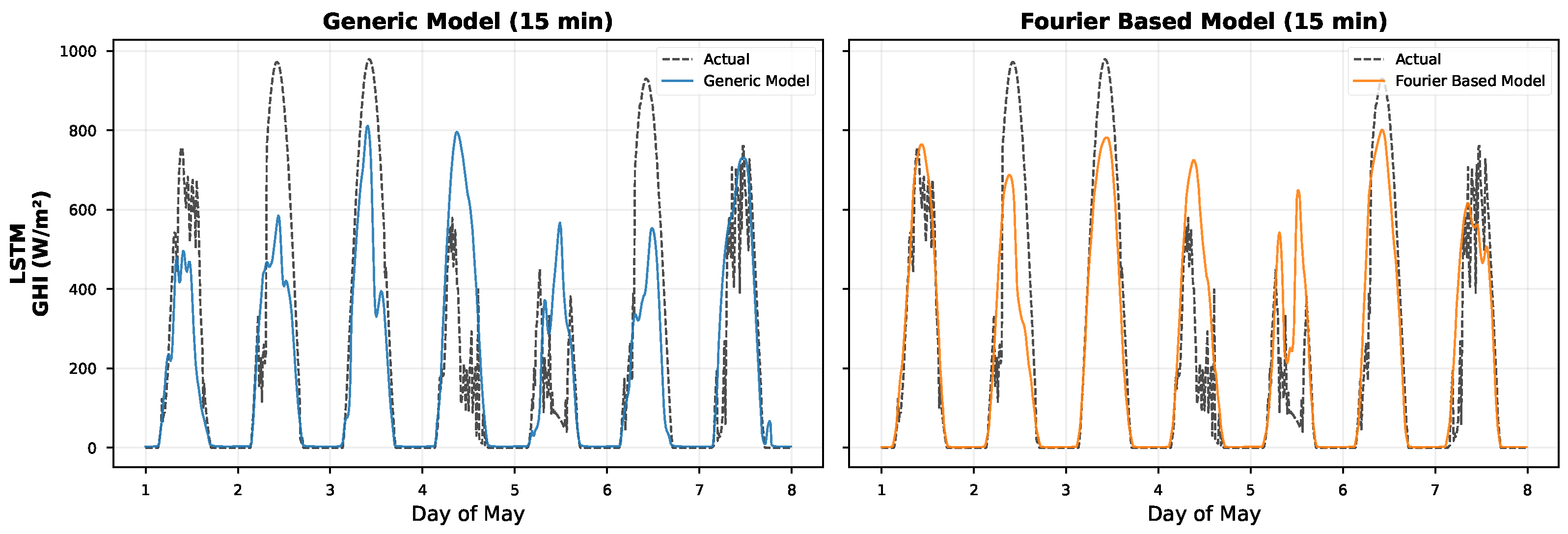
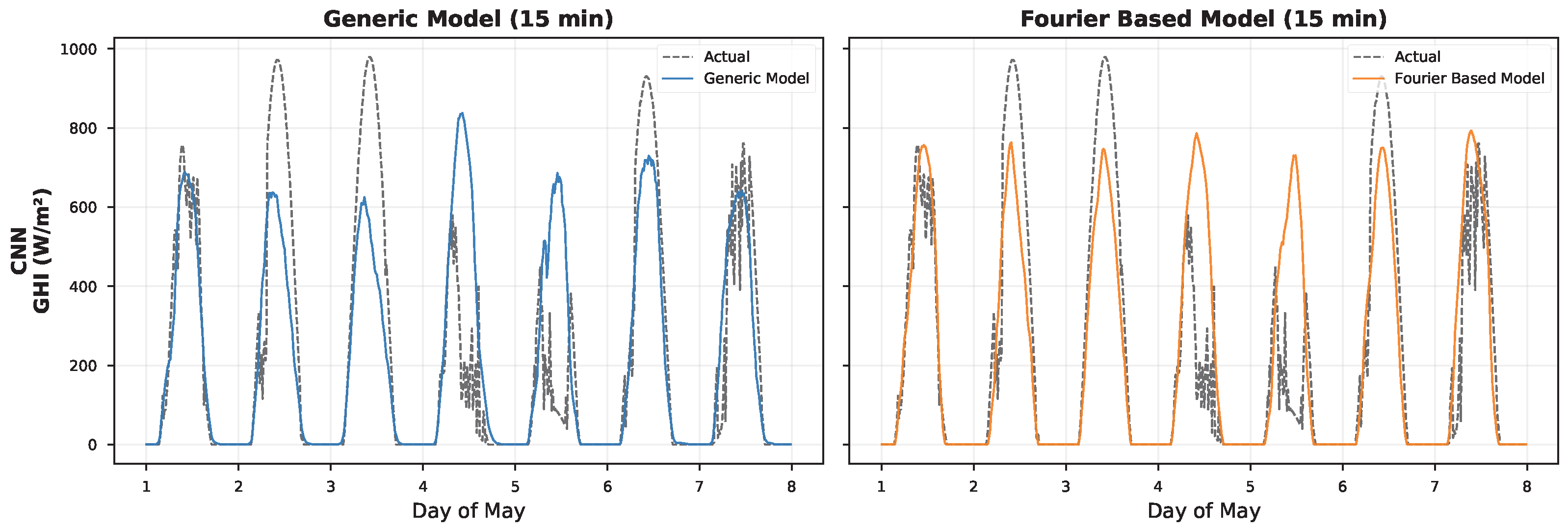
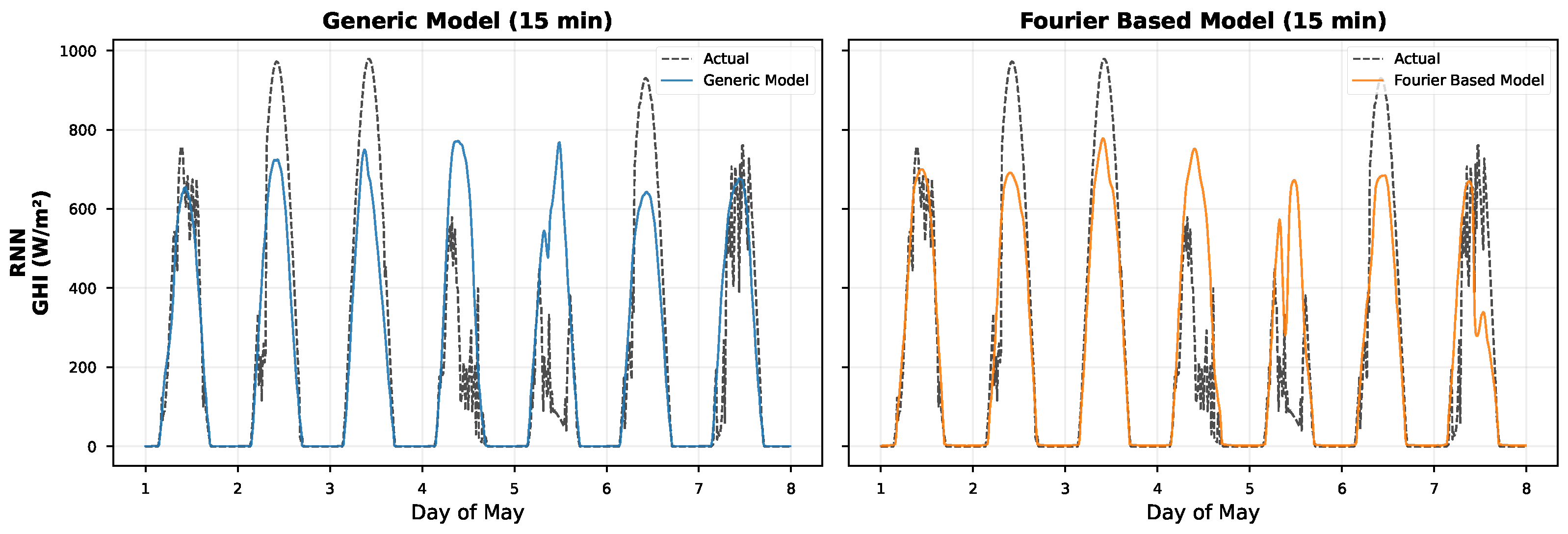
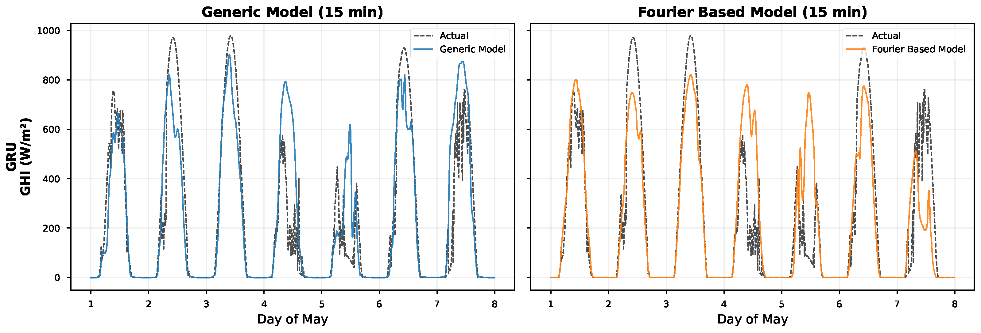
Figure 1, Figure 2, Figure 3 and Figure 4 show an interpretation of how well the models perform using visual representations of actual vs. predicted solar irradiance from the beginning of May, which is a time that often includes transitional weather patterns with both sunny and rainy days (and, thus, is an especially difficult time to predict). These plots represent two variants (“Fourier-Based” and “Generic”) to allow direct comparisons between the two.

5.1.1. Performance in Stable Conditions

Under clear sky conditions with relatively smooth, “bell shaped” irradiance profiles (i.e., those which closely resemble a sinusoidal function), all of the models demonstrated their ability to track the diel cycle. Both the generic and Fourier-based versions of the model were successful in modeling the sunrise, mid-day peak, and sunset phases. These results demonstrate that the baseline deep learning architectures used as a basis for these models are effective at extracting the low-frequency, periodic nature of solar data. While the two versions of the model had similar performance in terms of modeling the diel cycle, some differences existed in the smoothness of the modeled irradiance time series. The Fourier-based models generated much smoother time series in the middle of the day than the generic models did, effectively eliminating small-scale noise artifacts from the time series that were visible in the time series generated by the generic models.

5.1.2. Performance Under Volatility

This is where the Generic and Fourier-based approaches show their greatest differences. Most notably during the times that have occasional cloud cover and therefore rapidly changing levels of solar irradiance from one minute to another.

• RNN and GRU: The Generic RNN and Generic GRU had difficulty responding quickly to the rapid decline in irradiance due to clouds. The RNN and GRU with the Fourier layer were able to respond more quickly to these rapid declines in irradiance; they also responded to the subsequent recovery in irradiance (the rapid upswing). On the third day in Figure 2 the Fourier GRU was better able to capture the multi-modal aspects of the irradiance data than was the Generic GRU, whose output was a more smoothed average representation of the irradiance.
• CNN and LSTM: The CNN, well-known for extracting local temporal features of the data, improved uniformly when it was combined with the Fourier layer, as shown in Figure 4. The Fourier CNN also eliminated the “overshoot” common at the top of each spike in irradiance that occurred when clouds passed over. The Fourier-LSTM in Figure 3 showed the same level of improved stability as the CNN, eliminating the “phantom oscillations” that the Generic LSTMs sometimes would predict when the irradiance was zero (at night).

In summary, the qualitative results suggest that the addition of the Fourier layer enhanced the model’s ability to identify changes in the relevant signal variations and acted as a filter to eliminate irrelevant noise variations.

5.2. Quantitative Comparison of Performance

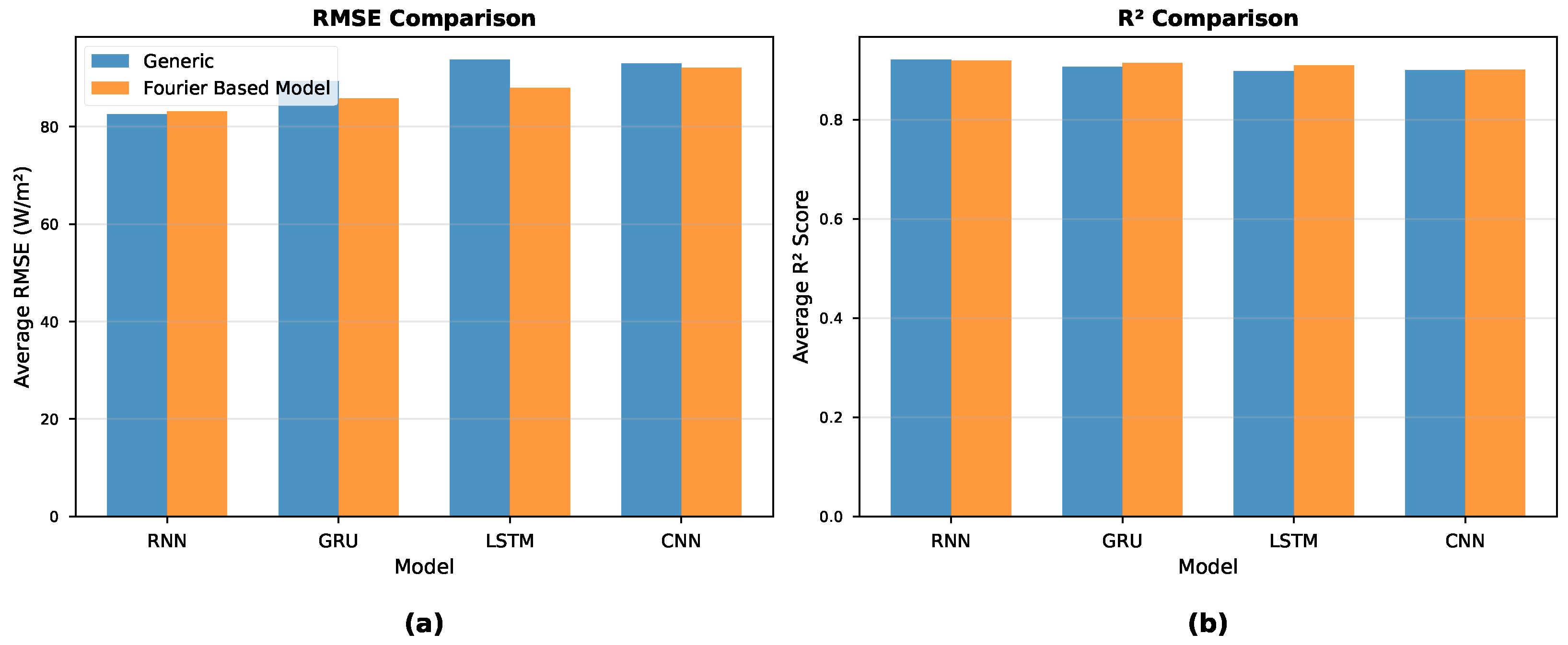
The quantitative results support our qualitative assessment. We evaluated the model under a wide range of scenarios using three different input window lengths ($w=\{24,48,96\}$) and four different forecast horizon lengths ($h=\{1,4,8,12\}$ time steps or, equivalently, 15, 60, 120, and 180 min). Figure 5 shows the average RMSE and average $R^2$ values for the Fourier-based models compared to the Generic models.

Detailed results for each model are provided in

Table 4. Extended Performance Metrics for GRU Generic.

Window Size	Horizon	RMSE	MAE	MSE	${\mathit{R}}^2$	Max. Error
24	1	84.20	35.17	7089.26	0.92	797.33
24	4	86.70	50.96	7516.65	0.91	798.54
24	8	92.32	39.07	8523.21	0.90	848.86
24	12	97.76	45.86	9557.04	0.89	817.86
48	1	84.58	38.46	7154.45	0.92	811.13
48	4	87.83	38.34	7714.61	0.91	781.71
48	8	85.77	36.83	7356.58	0.91	821.62
48	12	94.34	54.38	8899.82	0.90	849.25
96	1	85.36	36.67	7286.16	0.92	806.95
96	4	88.50	39.57	7832.64	0.91	836.73
96	8	91.98	45.34	8460.43	0.90	750.39
96	12	92.81	40.27	8613.14	0.90	785.37

,

Table 5. Extended Performance Metrics for GRU Fourier.

Window Size	Horizon	RMSE	MAE	MSE	${\mathit{R}}^2$	Max. Error
24	1	78.63	40.12	6182.18	0.93	706.10
24	4	84.83	44.32	7195.96	0.92	730.74
24	8	85.89	43.39	7377.73	0.91	732.66
24	12	86.37	40.25	7459.52	0.91	750.90
48	1	82.08	41.34	6737.01	0.92	749.25
48	4	80.87	42.39	6540.70	0.92	741.13
48	8	83.73	44.17	7011.12	0.92	665.52
48	12	92.66	45.88	8585.65	0.90	759.24
96	1	88.41	39.57	7816.91	0.91	757.01
96	4	86.23	45.10	7435.63	0.91	750.61
96	8	89.68	43.38	8041.96	0.91	836.57
96	12	89.61	41.89	8029.25	0.91	720.35

,

Table 6. Extended Performance Metrics for CNN Generic.

Window Size	Horizon	RMSE	MAE	MSE	${\mathit{R}}^2$	Max. Error
24	1	91.15	47.74	8308.67	0.90	797.32
24	4	88.20	45.07	7779.76	0.91	778.88
24	8	93.35	47.13	8713.53	0.90	719.70
24	12	97.30	47.83	9467.09	0.89	811.05
48	1	99.68	53.36	9936.76	0.88	796.96
48	4	89.62	45.86	8032.15	0.91	716.43
48	8	93.67	49.65	8773.51	0.90	722.00
48	12	94.96	47.20	9018.24	0.90	798.03
96	1	94.74	50.43	8975.58	0.90	724.35
96	4	89.56	46.44	8021.76	0.91	714.79
96	8	91.92	44.35	8448.82	0.90	759.34
96	12	91.79	44.52	8424.78	0.90	756.96

and

Table 7. Extended Performance Metrics for CNN Fourier.

Window Size	Horizon	RMSE	MAE	MSE	${\mathit{R}}^2$	Max. Error
24	1	83.56	40.58	6982.64	0.92	728.11
24	4	87.51	43.07	7657.42	0.91	691.65
24	8	90.50	46.71	8190.57	0.90	721.49
24	12	90.90	44.88	8263.26	0.90	743.26
48	1	87.36	44.36	7631.15	0.91	827.03
48	4	94.94	50.48	9013.68	0.90	720.15
48	8	91.74	46.68	8415.84	0.90	738.36
48	12	95.81	50.16	9179.97	0.89	716.95
96	1	88.67	45.35	7861.65	0.91	675.79
96	4	103.08	57.16	10625.84	0.88	716.62
96	8	93.52	45.90	8745.82	0.90	690.06
96	12	97.35	50.29	9476.25	0.89	685.05

.

5.2.1. Analysis of Gated Recurrent Units (GRUs)

The GRU architecture received the largest increase in performance after addition of the Fourier decomposition layer based on data presented in Table 4 and Table 5.

• Forecasting Short Horizons ($h=1$): For the smallest forecasting horizon (15 min), and window size of 24, the generic GRU performed poorly with an RMSE of 84.20 and $R^2$ of 0.917. By comparison, the GRU utilizing the Fourier decomposition layer produced an RMSE of 78.63 and an $R^2$ of 0.928, which is nearly six units less than the generic GRU, and demonstrates a substantial improvement in the precision of forecasts used immediately in dispatch decisions.
• Forecasting Longer Horizons ($h=12$): The importance of the spectral features were also demonstrated by their greater impact on longer forecast horizons. At $h=12$ (three hours ahead) with $w=24$, the Generic GRU degraded its performance to an RMSE of 97.76. However, the Fourier GRU retained much better stability in its performance, producing an RMSE of 86.37. Thus, the explicit modeling of periodic features within the Fourier layer help the GRU maintain its ability to capture important features over longer time intervals; this may be due in part to the reduced effect of the vanishing gradient problem present when making forecasts from long sequences of data.
• Effect of Window Size: While the Generic GRU’s RMSE decreased (from 95.04 to 85.36) and the RMSE increased (to 88.41) as the window size was increased to 96, it should be noted that the increase in RMSE does not necessarily indicate that longer context windows cannot be leveraged. Rather, the increase in RMSE indicates that the learning process was stabilized by the addition of the Fourier decomposition layer; this stabilization can lead to improved performance as additional data is added to the training set.

5.2.2. Convolutional Neural Network (CNN) Analysis

Convolutional neural networks (CNNs), by design, use localized receptive fields to extract spatially organized patterns within images; however, by adding a Fourier layer as a preprocessing step, we provided a CNN with global frequency information that can be used to enhance its ability to capture temporal patterns.

We believe that the CNN results shown in Table 6 and Table 7 demonstrate the complementary nature of frequency–domain and time–domain feature extraction.

• Synergistic Effect: Standard CNNs are designed to capture local patterns through their receptive field size. Adding the Fourier layer to the network, we have essentially provided the CNN with a global set of frequency descriptors that can be used to augment the local receptive field-based pattern capturing capabilities of the CNN. This synergy is demonstrated in the results obtained. Specifically, for a window length of $w=24$ and a horizon of $h=1$, the Generic CNN had an RMSE of 91.15, whereas the Fourier CNN had an RMSE of 83.56.
• Horizon Robustness: In general, as the horizon increases, the accuracy of the CNN will also degrade. The RMSE of the Generic CNN increased to 97.30 when the horizon was extended to $h=12$ (with $w=24$). Conversely, the RMSE of the Fourier CNN remained stable at 90.90 even after extending the horizon to $h=12$. Although still relatively high, these results show that the addition of frequency–domain interactions can serve as a “global anchor” to prevent the forecast from becoming increasingly inaccurate over longer horizons.

5.2.3. Recurrent Neural Network (RNN) Analysis

A Recurrent Neural Network (RNN) does not benefit from the additional frequency information to improve the RMSE of its predictions (

Table 8. Extended Performance Metrics for RNN Generic.

Window Size	Horizon	RMSE	MAE	MSE	${\mathit{R}}^2$	Max. Error
24	1	79.20	36.46	6273.24	0.93	777.87
24	4	79.73	38.34	6357.44	0.93	721.39
24	8	84.98	47.80	7221.53	0.92	739.84
24	12	87.14	40.06	7592.80	0.91	768.87
48	1	80.25	36.89	6439.81	0.93	775.31
48	4	80.31	42.24	6450.10	0.93	731.72
48	8	83.37	45.15	6951.28	0.92	795.85
48	12	87.38	46.98	7635.64	0.91	820.52
96	1	79.42	35.81	6308.32	0.93	782.29
96	4	80.57	37.42	6491.27	0.92	722.83
96	8	82.02	41.81	6727.75	0.92	787.96
96	12	86.41	42.53	7467.35	0.91	769.13

and

Table 9. Extended Performance Metrics for RNN Fourier.

Window Size	Horizon	RMSE	MAE	MSE	${\mathit{R}}^2$	Max. Error
24	1	79.84	39.67	6374.43	0.93	659.14
24	4	82.64	46.12	6828.90	0.92	631.37
24	8	84.17	43.62	7084.04	0.92	695.10
24	12	85.75	45.56	7352.70	0.91	714.88
48	1	81.45	43.34	6634.33	0.92	649.20
48	4	81.58	43.09	6654.85	0.92	641.48
48	8	86.63	44.60	7504.51	0.91	636.80
48	12	84.81	42.27	7192.36	0.92	691.58
96	1	80.79	40.23	6527.77	0.92	636.62
96	4	80.75	39.16	6519.83	0.92	652.24
96	8	83.74	44.25	7013.21	0.92	677.83
96	12	85.45	43.43	7302.13	0.92	629.20

); however, the RNN benefits significantly in terms of reliability.

• Consistency of Metrics: The Generic RNN and Fourier RNN showed comparable RMSE values of 79.20 and 79.84, respectively, when trained on data with a window length of $w=24$ and a horizon of $h=1$. The similar RMSE values suggest that for simple architectures such as the RNN, the learnable weights of the RNN alone are likely sufficient to identify the majority of the trends in the data.
• Extremely High Errors: However, the differences between the two models become apparent when examining the maximum error in the next section. While the RMSE of the two models are very close, the maximum errors in each model are quite different. The Fourier RNN has a much lower probability of making large mistakes in predicting future values.

5.2.4. Long Short-Term Memory (LSTM) Analysis

The Long Short-Term Memory (LSTM) is currently the most widely used architecture in the deep learning community for solving many time series forecasting problems (

Table 10. Extended Performance Metrics for LSTM Generic.

Window Size	Horizon	RMSE	MAE	MSE	${\mathit{R}}^2$	Max. Error
24	1	83.81	43.78	7024.72	0.92	862.55
24	4	90.16	60.28	8129.43	0.91	767.96
24	8	101.92	68.75	10387.10	0.88	812.46
24	12	102.37	61.49	10479.26	0.88	807.42
48	1	91.47	58.64	8366.99	0.90	780.20
48	4	89.03	58.45	7926.33	0.91	792.47
48	8	94.36	55.62	8903.42	0.90	822.35
48	12	96.86	59.59	9380.90	0.89	798.17
96	1	91.70	46.65	8408.64	0.90	816.94
96	4	92.72	61.34	8596.49	0.90	821.03
96	8	90.55	54.36	8199.72	0.90	799.06
96	12	99.63	53.01	9925.93	0.88	870.75

and

Table 11. Extended Performance Metrics for LSTM Fourier.

Window Size	Horizon	RMSE	MAE	MSE	${\mathit{R}}^2$	Max. Error
24	1	86.86	39.63	7543.89	0.91	835.52
24	4	85.87	43.34	7374.30	0.91	835.64
24	8	86.55	39.93	7490.13	0.91	730.89
24	12	89.34	42.97	7980.99	0.91	760.43
48	1	84.06	39.44	7065.66	0.92	741.43
48	4	87.42	42.81	7641.73	0.91	759.06
48	8	87.30	44.62	7620.83	0.91	702.67
48	12	87.63	43.48	7678.69	0.91	774.68
96	1	84.35	42.26	7114.64	0.92	752.55
96	4	88.22	42.29	7783.19	0.91	699.66
96	8	91.78	42.90	8423.87	0.90	847.66
96	12	96.06	48.63	9228.38	0.89	826.74

).

• Incremental Improvement: When comparing the performance of the Reference LSTM model trained using $w=96$ and $h=1$ to the performance of the Fourier LSTM model trained using $w=96$ and $h=1$, we see that the Reference LSTM model had an RMSE of 91.70, and the Fourier LSTM model had an RMSE of 84.35. The percentage improvement of the Fourier LSTM model compared to the Reference LSTM model is slightly lower than the improvements seen in the GRU models but is consistent across nearly every window size examined.
• Handling Complex Relationships: The LSTMs’ gate functions allow them to effectively capture relationships in the time domain. With the addition of the Fourier features to the LSTM model, the burden of identifying and tracking simple periodicities such as the daily/nightly cycle can be shifted to the input layer of the LSTM model. Thus, the LSTM gates can focus on identifying the complex, nonlinear, and stochastic cloud variances. The hypothesis that the inclusion of Fourier features would result in improved MAE scores is supported by the results obtained. The MAE score decreased from 46.65 (Generic) to 42.26 (Fourier) when training both the Generic and Fourier LSTMs on data with a window length of $w=96$ and a horizon of $h=1$.

5.3. Error Analysis and Robustness

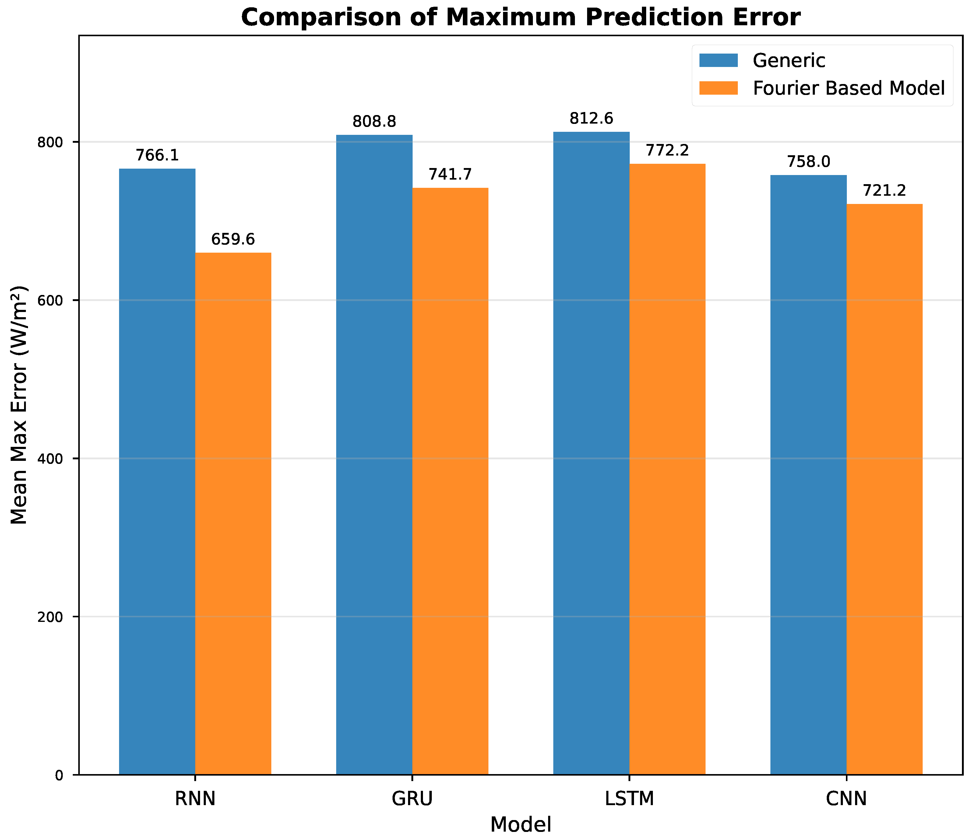
A very important yet often ignored component of forecasting models for energy grids is the reliability of these models. A model with a low average prediction error but occasional large errors can be extremely harmful to the overall stability of an energy grid. We measured this by analyzing the Mean Maximum Prediction Error (Max Error) illustrated graphically in Figure 6.

The results are unequivocal: the Fourier-based models are significantly more robust.

1.

Drastic Reduction in Outliers: The Generic models frequently exhibited Max Errors in the range of 800–900 W/m². For instance, the Generic GRU ($w=24,h=1$) had a Max Error of 797.33. The Fourier-based GRU reduced this peak error to 706.10.

2.

RNN Stability: The Generic RNN ($w=24,h=1$) suffered a Max Error of 777.87. The Fourier RNN cut this down to 659.14. This is a massive improvement, indicating that while the average performance (RMSE) was similar, the worst-case performance of the Fourier model is far superior.

3.

Consistency Across Scales: This trend of reduced Max Error is observed across nearly every combination of model variability, window size, and horizon. It suggests that the Fourier decomposition acts as a regularizer, preventing the model from “chasing” noise or reacting excessively to sensor anomalies. By grounding the predictions in the fundamental frequencies of the signal, the model is constrained to physically plausible manifolds, thereby capping the magnitude of erroneous predictions.

5.4. Computational Efficiency

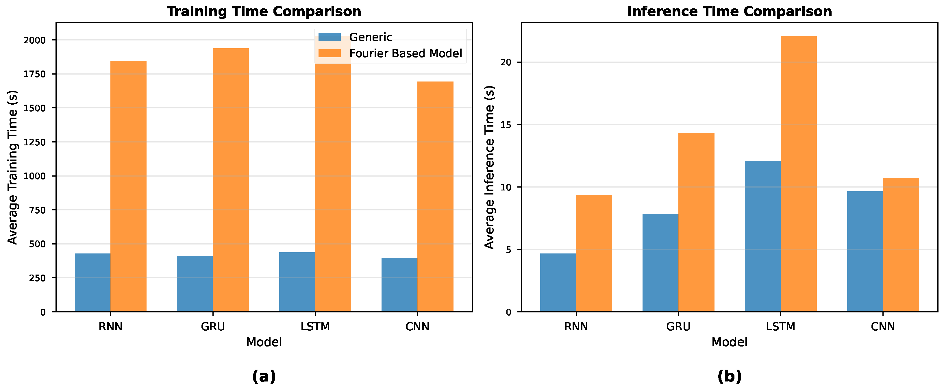
Practical use of deep learning models to be used for the design of smart grids has to take into account the trade-off between accuracy and computational cost. We present the efficiency comparison of our proposed models in Figure 7.

• Training Time: Training times are very similar to the original model. The Fast Fourier Transform (FFT) used in the Fourier models and the additional parameters added in the concatenated layers add a small amount of overhead. Because we are considering the training process as being performed during off-line periods, these increases are irrelevant.
• Inference Time: Most importantly, inference time is still very low. The FFT has been highly optimized by modern hardware. As such, the increase in inference latency is in the order of milliseconds. This is also acceptable for the majority of real-time grid control systems with typical dispatch cycle of 15 min or 5 min.

5.5. Training Performance of Models

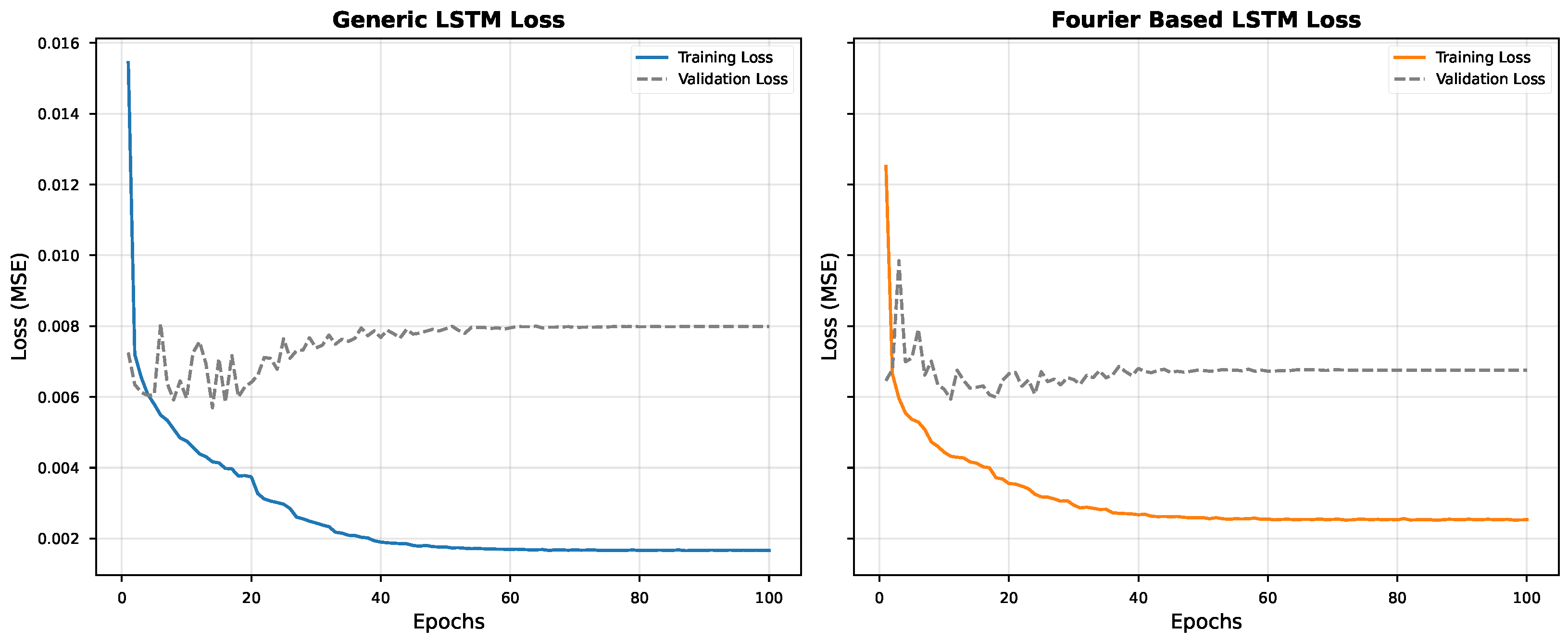
The plots of the training loss and validation loss versus number of epochs for both Generic and Fourier based LSTM are shown in Figure 8. This depicts how well each model learns from the training data (i.e., fits to the training data). We see that the Fourier-based model has a faster and more regular convergence than the generic model. This rapid convergence to a constant value can be attributed to the pre-defined knowledge of frequency in the Fourier-based model. That is, when we use a Fourier transform on an input signal, we know beforehand that this will represent the frequency information as a function of time or location, which allows the optimization algorithm to search the parameter space with less uncertainty and, therefore, with more efficiency. In addition to faster convergence, we also observe that the difference between the validation loss and training loss are smaller for the Fourier-based model, which indicates better generalization capabilities of the Fourier-based model and a lower probability of fitting to the noise in the training data.

5.6. Broad Impact

The results from this research have broad implications for the renewable energy industry. The addition of physics-aware interpretable layers into “black box” DL models improves the reliability of those models.

1.

Grid Reliability: Reduced maximum error represents reduced risk to grid operators. This means that with lower worst-case forecast errors, there will be fewer reserve requirements to pay for and fewer instances where expensive spinning reserve has to be dispatched.

2.

Interpretation: With the capability of determining which frequency bands contribute to specific forecasts (using the architecture), we move one step closer to Explainable AI (XAI) for energy.

3.

Generalization: While developed using solar irradiance data, this methodology is applicable to other periodic time series usage profiles (e.g., electricity load demand; wind speed forecasting).

Overall, this Fourier-based methodology provides models that are both more accurate on average (i.e., lower RMSE/MAE) and more reliable and safe (i.e., lower Max Error) than traditional methodologies when it comes to critical infrastructure applications.

6. Conclusions and Future Research

In this paper we have developed an interpretable deep learning framework for the prediction of solar irradiance, which is based on a Fourier decomposition of the signal together with a convolutional neural network (CNN). Both, the prediction quality of our method, as well as its interpretability, are crucial for solar-energy-related applications. The major contributions of this work are as follows:

1.

Physics-Aware Signal Decomposition: We introduced a new decomposition method of the solar irradiance signal, which divides the signal into trend, seasonal, and residual components, using polynomial and Fourier-based functions. Our decomposition has a clear relation to the physical processes influencing solar radiation and, therefore, allows us to apply special methods for every single component.

2.

Comparison of Architectures: In order to determine the most suitable architecture among the given four architectures (RNN, LSTM, GRU, CNN), we performed a systematic comparison of the architectures within the two categories, namely (a) generic architectures and (b) Fourier-based architectures, resulting in a total number of $3\times 4\times 8=96$ experiments with varying combinations of three window sizes and four prediction horizons.

3.

Improved Interpretability: The three-stack architecture provides insight into how every single component contributes to the final prediction and, thus, offers a possibility for the validation of predictions made by a domain expert.

We found that the Fourier-based GRU achieved the best performance over all architectures with respect to both Root Mean Squared Error (RMSE = 78.63 W/m²) and Coefficient of Determination ($R^2=0.9281$) at the best configuration of the parameter set (window size: 6 h (24 steps); prediction horizon: 15 min). The finding that simpler architectures (RNN, GRU) outperformed the more complex LSTM warrants discussion. We hypothesize that the Fourier-based signal decomposition effectively removes the deterministic periodic components from the input signal, leaving a residual that is more stationary and exhibits shorter-term dependencies. This preprocessing step reduces the need for the sophisticated gating mechanisms in LSTMs, which are designed to selectively remember or forget information over long sequences. When the long-term periodic structure is explicitly modeled by the Fourier basis, the simpler gating structures of GRUs (or even vanilla RNNs) are sufficient to model the remaining stochastic variations, while the additional parameters in LSTMs may lead to overfitting on the residual component. Among the recurrent architectures, we also find that RNN and GRU achieved the highest prediction accuracy, whereas LSTM showed a slightly worse performance. The CNN–Fourier model (RMSE = 83.56 W/m²; R² = 0.9188) performed competitively and even better than the two LSTM variants. Compared to their generic counterparts, the Fourier-based models of this study show the same or even better prediction accuracy, but they provide the additional benefit of being understandable. Furthermore, we found that the Fourier-based GRU outperformed the generic GRU by 6.6% in terms of RMSE, and the Fourier-based LSTM outperformed the generic LSTM by 8.0%. As expected, the models suffer from a predictable degradation of prediction accuracy when increasing the prediction horizon. Specifically, the R² values decrease from about 0.93 at prediction horizons of 15 min to about 0.87 at horizons of 3 h.

Future Research Directions

There are some interesting possibilities for further research based on the findings and limitations of this study. A limitation of the current work is the focus on comparing Fourier-based models against their generic counterparts without including classical baselines such as persistence (last-value) forecasting, linear regression, or traditional machine learning methods (SVR and gradient boosting). Future work should include these baselines to provide a more comprehensive performance context. For instance, we could combine multiple Fourier-based models by applying ensemble methods so as to increase both prediction accuracy and the robustness of uncertainty estimation. Another possible direction of research is to develop incremental learning strategies, allowing models to adapt to changing atmospheric conditions and sensor drift without full re-training. Additionally, we may expand the scope of our framework to enable simultaneous prediction of multiple future time steps, thereby generating comprehensive forecasting profiles for energy scheduling applications.

References

1. Sobri, S.; Koohi-Kamali, S.; Rahim, N.A. Solar photovoltaic generation forecasting methods: A review. Energy Convers. Manag. 2018, 156, 459–497. [Google Scholar] [CrossRef]
2. Singla, P.; Duhan, M.; Saroha, S. Review of Different Error Metrics: A Case of Solar Forecasting. AIUB J. Sci. Eng. 2021, 20, 158–165. [Google Scholar] [CrossRef]
3. Voyant, C.; Notton, G.; Kalogirou, S.; Nivet, M.L.; Paoli, C.; Motte, F.; Fouilloy, A. Machine learning methods for solar radiation forecasting: A review. Renew. Energy 2017, 105, 569–582. [Google Scholar] [CrossRef]
4. Diagne, M.; David, M.; Lauret, P.; Boland, J.; Schmutz, N. Review of solar irradiance forecasting methods and a proposition for small-scale insular grids. Renew. Sustain. Energy Rev. 2013, 27, 65–76. [Google Scholar] [CrossRef]
5. Mellit, A.; Massi Pavan, A.; Ogliari, E.; Leva, S.; Lughi, V. Advanced Methods for Photovoltaic Output Power Forecasting: A Review. Appl. Sci. 2020, 10, 487. [Google Scholar] [CrossRef]
6. Kihtir, F.; Oztoprak, K. Deep FS: A Deep Learning Approach for Surface Solar Radiation. Sensors 2024, 24, 8059. [Google Scholar] [CrossRef]
7. Li, H.; Wu, W.; Chen, W.; Zhang, M. RTI-Net: Physics-informed deep learning for photovoltaic power forecasting. Renew. Energy 2026, 256, 124152. [Google Scholar] [CrossRef]
8. Yan, K.; Shen, H.; Wang, L.; Zhou, H.; Xu, M.; Mo, Y. Short-Term Solar Irradiance Forecasting Based on a Hybrid Deep Learning Methodology. Information 2020, 11, 32. [Google Scholar] [CrossRef]
9. Hochreiter, S.; Schmidhuber, J. Long Short-Term Memory. Neural Comput. 1997, 9, 1735–1780. [Google Scholar] [CrossRef] [PubMed]
10. Jang, S.Y.; Oh, B.T.; Oh, E. A Deep Learning-Based Solar Power Generation Forecasting Method Applicable to Multiple Sites. Sustainability 2024, 16, 5240. [Google Scholar] [CrossRef]
11. Cho, K.; van Merriënboer, B.; Gulcehre, C.; Bahdanau, D.; Bougares, F.; Schwenk, H.; Bengio, Y. Learning Phrase Representations using RNN Encoder–Decoder for Statistical Machine Translation. In Proceedings of the 2014 Conference on Empirical Methods in Natural Language Processing (EMNLP), Doha, Qatar, 25–29 October 2014; pp. 1724–1734. [Google Scholar] [CrossRef]
12. Bashir, T.; Wang, H.; Tahir, M.; Zhang, Y. Wind and solar power forecasting based on hybrid CNN-ABiLSTM, CNN-transformer-MLP models. Renew. Energy 2025, 239, 122055. [Google Scholar] [CrossRef]
13. Feng, C.; Zhang, J.; Zhang, W.; Hodge, B.M. Convolutional neural networks for intra-hour solar forecasting based on sky image sequences. Appl. Energy 2022, 310, 118438. [Google Scholar] [CrossRef]
14. Lin, Y.; Koprinska, I.; Rana, M. Temporal Convolutional Neural Networks for Solar Power Forecasting. In Proceedings of the 2020 International Joint Conference on Neural Networks (IJCNN), Glasgow, UK, 19–24 July 2020; pp. 1–8. [Google Scholar] [CrossRef]
15. Lim, S.C.; Huh, J.H.; Hong, S.H.; Park, C.Y.; Kim, J.C. Solar Power Forecasting Using CNN-LSTM Hybrid Model. Energies 2022, 15, 8233. [Google Scholar] [CrossRef]
16. Guo, W.; Liu, S.; Weng, L.; Liang, X. Power Grid Load Forecasting Using a CNN-LSTM Network Based on a Multi-Modal Attention Mechanism. Appl. Sci. 2025, 15, 2435. [Google Scholar] [CrossRef]
17. Khan, A.A.A.; Ullah, M.H.; Tabassum, R.; Kabir, M.F. Enhanced Transformer-BiLSTM Deep Learning Framework for Day-Ahead Energy Price Forecasting. IEEE Trans. Ind. Appl. 2025; in press. [Google Scholar] [CrossRef]
18. Lei, C.; Zhang, H.; Wang, Z.; Miao, Q. Deep Learning for Demand Forecasting: A Framework Incorporating Variational Mode Decomposition and Attention Mechanism. Processes 2025, 13, 594. [Google Scholar] [CrossRef]
19. Boucetta, L.N.; Amrane, Y.; Chouder, A.; Arezki, S.; Kichou, S. Enhanced Forecasting Accuracy of a Grid-Connected Photovoltaic Power Plant: A Novel Approach Using Hybrid Variational Mode Decomposition and a CNN-LSTM Model. Energies 2024, 17, 1781. [Google Scholar] [CrossRef]
20. Kim, D.H.; Kim, D.J.; Choi, S.Y. A Variational-Mode-Decomposition-Cascaded Long Short-Term Memory with Attention Model for VIX Prediction. Appl. Sci. 2025, 15, 5630. [Google Scholar] [CrossRef]
21. Xiao, Z.; Li, C.; Hao, H.; Liang, S.; Shen, Q.; Li, D. VBTCKN: A Time Series Forecasting Model Based on Variational Mode Decomposition with Two-Channel Cross-Attention Network. Symmetry 2025, 17, 1063. [Google Scholar] [CrossRef]
22. Xu, C.; Li, C.; Zhou, X. Interpretable LSTM Based on Mixture Attention Mechanism for Multi-Step Residential Load Forecasting. Electronics 2022, 11, 2189. [Google Scholar] [CrossRef]
23. Ranjan, P.; Itani, R.; Faccia, A. An Interpretable 1D-CNN Framework for Stock Price Forecasting: A Comparative Study with LSTM and ARIMA. FinTech 2025, 4, 63. [Google Scholar] [CrossRef]
24. Sengupta, M.; Xie, Y.; Habte, A.; Buster, G.; Maclaurin, G.; Edwards, P.; Sky, H.; Bannister, M.; Rosenlieb, E. The National Solar Radiation Database (NSRDB) Fiscal Years 2019–2021 (Final Report); Technical Report; National Renewable Energy Laboratory (NREL): Golden, CO, USA, 2022. [CrossRef]
25. Khalil, R.; Hollweg, G.V.; Hussain, A.; Su, W.; Bui, V.H. Assessment of Solar Energy Generation Toward Net-Zero Energy Buildings. Algorithms 2024, 17, 528. [Google Scholar] [CrossRef]
26. Xu, Q.; Zhang, Z.; Wang, G.; Chen, Y. Explainable Multi-Scale CAM Attention for Interpretable Cloud Segmentation in Astro-Meteorological Applications. Appl. Sci. 2025, 15, 8555. [Google Scholar] [CrossRef]
27. Mauladdawilah, H.; Balfaqih, M.; Balfagih, Z.; Pegalajar, M.d.C.; Gago, E.J. Deep Feature Selection of Meteorological Variables for LSTM-Based PV Power Forecasting in High-Dimensional Time-Series Data. Algorithms 2025, 18, 496. [Google Scholar] [CrossRef]
28. Arafet, K.; Berlanga, R. Digital Twins in Solar Farms: An Approach through Time Series and Deep Learning. Algorithms 2021, 14, 156. [Google Scholar] [CrossRef]
29. Garagnani, F.; Maniezzo, V. Deconstructing a Minimalist Transformer Architecture for Univariate Time Series Forecasting. Algorithms 2025, 18, 645. [Google Scholar] [CrossRef]
30. Zhang, H.; Li, B.; Su, S.F.; Yang, W.; Xie, L. A Novel Hybrid Transformer-Based Framework for Solar Irradiance Forecasting Under Incomplete Data Scenarios. IEEE Trans. Ind. Inform. 2024, 20, 8605–8615. [Google Scholar] [CrossRef]
31. Haljasmaa, K.I.; Bramm, A.M.; Matrenin, P.V.; Eroshenko, S.A. Weather Condition Clustering for Improvement of Photovoltaic Power Plant Generation Forecasting Accuracy. Algorithms 2024, 17, 419. [Google Scholar] [CrossRef]
32. Lin, K.H.; Hsu, P.Y.; Chen, P.H.; Chen, M.Y. A Novel Framework for Solar Irradiance Prediction Integrating Signal Decomposition With Hybrid Time-Series Models. IEEE Access 2025, 13, 123414–123428. [Google Scholar] [CrossRef]
33. Kim, W.W.; Kim, J.H. Multi-Resolution LSTNet Framework with Wavelet Decomposition and Residual Correction for Long-Term Hourly Load Forecasting on Distribution Feeders. Energies 2025, 18, 5385. [Google Scholar] [CrossRef]
34. Liu, Y.; Yang, M. Ultra-Short-Term Photovoltaic Power Prediction Based on Predictable Component Reconstruction and Spatiotemporal Heterogeneous Graph Neural Networks. Energies 2025, 18, 4192. [Google Scholar] [CrossRef]
35. Mchara, W.; Manai, L.; Abdellatif Khalfa, M.; Raissi, M.; Hannechi, S. A Global Irradiance Prediction Model Using Convolutional Neural Networks, Wavelet Neural Networks, and Masked Multi-Head Attention Mechanism. IEEE Access 2025, 13, 29445–29462. [Google Scholar] [CrossRef]
36. Zheng, D.; Qin, J.; Liu, Z.; Zhang, Q.; Duan, J.; Zhou, Y. BWO–ICEEMDAN–iTransformer: A Short-Term Load Forecasting Model for Power Systems with Parameter Optimization. Algorithms 2025, 18, 243. [Google Scholar] [CrossRef]
37. Hu, X. Weather Phenomena Monitoring: Optimizing Solar Irradiance Forecasting With Temporal Fusion Transformer. IEEE Access 2024, 12, 194133–194149. [Google Scholar] [CrossRef]
38. Barancsuk, L.; Groma, V.; Kocziha, B. Hybrid ultra-short term solar irradiation forecasting using resource-efficient multi-step long-short term memory. Renew. Energy 2025, 247, 122962. [Google Scholar] [CrossRef]
39. Wang, C.; Wang, H.; Bi, J.; Yan, K. Short-Term Solar Irradiance Forecasting Based on CNNiTransformer Model. In Proceedings of the 2024 IEEE Cyber Science and Technology Congress (CyberSciTech), Malay, Philippines, 5–8 November 2024; pp. 174–179. [Google Scholar] [CrossRef]
40. Zi, X.; Liu, F.; Liu, M.; Wang, Y. Transformer with Adaptive Sparse Self-Attention for Short-Term Photovoltaic Power Generation Forecasting. Electronics 2025, 14, 3981. [Google Scholar] [CrossRef]
41. Huang, X.; Ding, X.; Han, Y.; Sima, Q.; Li, X.; Bao, Y. Day-Ahead Photovoltaic Power Forecasting Based on SN-Transformer-BiMixer. Energies 2025, 18, 4406. [Google Scholar] [CrossRef]
42. Chiranjeevi, M.; Moger, T.; Jena, D. Solar Irradiance Forecasting Performance Enhancement Using Hybrid Fuzzy-Based CNN-BiLSTM-Transformer Model. IEEE Access 2025, 13, 186795–186810. [Google Scholar] [CrossRef]
Figure 1. RNN: Actual vs. Predicted Solar Irradiance. Comparison of Generic model (Left) vs. Fourier-Based model (Right).
Algorithms 19 00081 g001
Figure 2. GRU: Actual vs. Predicted Solar Irradiance. Comparison of Generic model (Left) vs. Fourier-Based model (Right).
Algorithms 19 00081 g002
Figure 3. LSTM: Actual vs. Predicted Solar Irradiance. Comparison of Generic model (Left) vs. Fourier-Based model (Right).
Algorithms 19 00081 g003
Figure 4. CNN: Actual vs. Predicted Solar Irradiance. Comparison of Generic model (Left) vs. Fourier-Based model (Right).
Algorithms 19 00081 g004
Figure 5. Average Performance Comparison. (a) RMSE Comparison across all models; (b) R 2 Comparison across all models.
Algorithms 19 00081 g005
Figure 6. Comparison of Maximum Absolute Prediction Error across all models.
Algorithms 19 00081 g006
Figure 7. Computational Efficiency Comparison: (a) Training Time and (b) Inference Time. Note: Inference times shown represent total dataset inference time for the complete test set (approximately 35,000 samples), not per-sample latency. Per-sample latency can be computed by dividing by the number of test samples, yielding sub-millisecond inference times suitable for real-time applications.
Algorithms 19 00081 g007
Figure 8. Training and Validation Loss for Generic LSTM vs. Fourier-Based LSTM.
Algorithms 19 00081 g008