Article

Decision-Time Learning and Planning Integrated Control for the Mild Hyperbaric Chamber

School of Mechanical Engineering, Xi’an Jiaotong University, Xi’an 710049, China
*
Author to whom correspondence should be addressed.
Algorithms 2025, 18(7), 380; https://doi.org/10.3390/a18070380
Submission received: 30 May 2025 / Revised: 18 June 2025 / Accepted: 20 June 2025 / Published: 23 June 2025
(This article belongs to the Special Issue Algorithmic Approaches to Control Theory and System Modeling)

Abstract

Plateau hypoxia represents a type of hypobaric hypoxia caused by reduced atmospheric pressure at high altitudes. Pressurization therapy is one of the most effective methods for alleviating acute high-altitude sickness. This study focuses on the development of an advanced control system for a vehicle-mounted mild hyperbaric chamber (MHBC) designed for the prevention and treatment of plateau hypoxia. Conventional control methods struggle to cope with the high complexity and inherent uncertainties associated with MHBC control tasks, thereby motivating the exploration of sequential decision-making approaches such as reinforcement learning. Nevertheless, the application of sequential decision-making in MHBC control encounters several challenges, including data inefficiency and non-stationary dynamics. The system’s low tolerance for trial-and-error may lead to component damage or unsafe operating conditions, and anomalies such as valve failure can emerge during long-term operation, compromising system stability. To address these challenges, this study proposes a decision-time learning and planning integrated framework for MHBC control. Specifically, an innovative latent model embedding decision-time learning is designed for system identification, separately managing system uncertainties to fine-tune the model output. Furthermore, a decision-time planning algorithm is developed and the planning process is further guided by incorporating a value network and an enhanced online policy. Experimental results demonstrate that the proposed decision-time learning and planning integrated approaches achieve notable performance in MHBC control.

1. Introduction

The environmental conditions of plateau regions are characterized by low air density and reduced oxygen concentration. As altitude increases, atmospheric pressure progressively decreases, leading to a corresponding decline in the partial pressure of oxygen in the air, thereby creating severe hypoxia conditions in high-altitude regions. This hypoxic condition exerts detrimental effects on multiple physiological systems, including the nervous, respiratory, and circulatory systems, and is the primary cause of altitude-related illnesses. When the human body is exposed to high-altitude hypoxia, inadequate oxygen supply can induce acute altitude reactions such as headaches, dizziness, and nausea. In severe cases, it may even lead to life-threatening conditions such as high-altitude pulmonary edema or high-altitude cerebral edema.
Hyperbaric oxygen therapy (HBOT) has emerged as one of the most effective methods for both preventing and treating altitude sickness [1]. By allowing patients to breathe high-concentration oxygen in an environment with pressure higher than one atmosphere, HBOT increases blood oxygen content and improves tissue oxygenation. Compared to oxygen inhalation under atmospheric conditions, the elevated ambient pressure and oxygen partial pressure provided by HBOT can significantly increase the dissolved oxygen content in blood and tissues for several hours after therapy ends, thereby mitigating hypoxic damage. This therapy has achieved promising results in the treatment of hypoxic diseases and emergency intervention for altitude sickness. The core device facilitating HBOT is the hyperbaric chamber, which provides a sealed high-pressure, high-oxygen environment for therapeutic purposes. However, conventional hyperbaric chambers present limitations due to their large-scale, complex, and costly nature, requiring specialized facilities and skilled personnel, thus rendering them unsuitable for widespread use in high-altitude regions.
To address this limitation, we have developed a more practical solution as the mild hyperbaric chamber (MHBC). Evolved from traditional hyperbaric chamber technology, the MHBC represents an innovative pressurized oxygen-enriched device specifically designed to offer accessible and comfortable oxygen therapy for both residents and travelers in high-altitude areas. Unlike hyperbaric chambers in hospital, the operating pressure of an MHBC is relatively slightly elevated above ambient levels (typically less than 0.6 atm). This modest pressure differential significantly reduces structural requirements and associated safety considerations, enabling a more compact and lightweight design. This feature facilitates mobile deployment, including vehicle-mounted configurations, improving portability and usability. As shown in Figure 1, the vehicle-mounted plateau MHBC incorporates an integrated design where the pressurization chamber and auxiliary power system are housed within a single modular enclosure. The chamber is secured onto the vehicle chassis using a bolted frame structure, constituting a mobile oxygen therapy unit. The MHBC establishes a comfortable, efficient, and readily accessible oxygen-enriched environment, effectively mitigating hypoxia-related health issues in high-altitude regions and emerging as one of the most effective approaches for the prevention and treatment of altitude sickness.
This study focuses on the control system design for the MHBC. In the field of medical hyperbaric oxygen chambers, extensive research has been conducted on the development of automated control systems to improve treatment conditions, enhance control accuracy and system stability, and ultimately optimize therapeutic outcomes. For example, Lefebvre et al. designed a novel bench-test ventilator for hyperbaric chambers to accommodate pressure regulation under varying atmospheric conditions [2]. De Paco et al. developed an automated multi-place hyperbaric oxygen therapy system, significantly enhancing patient comfort and safety while reducing the incidence of barotrauma [3]. Wang et al. proposed a hypoxic chamber control system based on a fuzzy adaptive control algorithm, which integrates expert and proportional–derivative control strategies to effectively address time delay and uncertainty in the chamber environment [4]. Gracia et al. achieved the automation of a multi-place hyperbaric chamber using a zero-pole cancellation regulator, ensuring accurate pressure tracking and repeatability, and successfully deployed the system in a clinical setting [5]. Motorga et al. developed an adaptive PID controller based on artificial intelligence for pressure regulation in surgical hyperbaric chambers, significantly improving system responsiveness, although challenges such as pressure overshoot and disturbance rejection remain unresolved [6]. Most existing studies adopt PID or fuzzy control strategies, which generally offer limited control precision and inadequate disturbance rejection capabilities. Furthermore, these approaches often lack a systematic consideration of the various factors influencing pressure variation. With the advent of the era of artificial intelligence, medical devices are increasingly evolving toward intelligent and user-centric systems. In the context of hyperbaric chamber usage, users are becoming increasingly concerned not only with treatment efficacy but also with the comfort and convenience of the therapeutic experience.
Over the past decade, machine learning and deep learning-based technologies have rapidly developed, playing an increasingly significant role in daily life. As a subfield of machine learning, Reinforcement learning (RL) has gained increasing attention due to its ability to handle sequential decision-making problems [7]. RL represents the third category of machine learning, alongside supervised learning and unsupervised learning. Since the 1980s, classical RL methods have been continuously developed. With advancements in deep learning, RL has entered a phase of accelerated growth. In 2016, Google DeepMind leveraged Monte Carlo Tree Search (MCTS) to develop AlphaGo, which ultimately defeated the reigning world champion in Go, generating widespread interest [8]. By 2023, RL had been extensively applied in training large language models such as ChatGPT, where Reinforcement Learning from Human Feedback (RLHF) was used to fine-tune responses based on human evaluations [9]. Currently, RL is widely applied in robotics, game intelligence, smart cities, recommendation systems, and energy optimization, demonstrating immense potential. In recent years, RL has attracted growing interest in process control applications, primarily due to its capability to handle high-dimensional nonlinear systems, time-varying environments, and constraint optimization problems. By interacting with the environment to learn optimal policies, RL enables intelligent agents to maximize cumulative rewards in multi-step decision-making processes. This provides an intelligent control approach that overcomes the limitations of traditional control methods.
However, the primary challenges of applying reinforcement learning methods to the control of MHBC include data efficiency and non-stationary dynamics. On one hand, reinforcement learning methods rely on extensive interaction data and an iterative trial-and-error mechanism to optimize policies. In the control scenario of MHBC, frequent experimental interactions may cause damage to critical components such as control valves. Additionally, due to the high-pressure and enclosed nature of the MHBC environment, entering an abnormal state during the trial-and-error process could pose serious threats to system safety. On the other hand, during long-time operation, MHBC is prone to abnormal conditions such as valve failure. If the controller fails to adjust the control in time, the system pressure may deviate from normal range, jeopardizing the stability and safety of the system. Modern control systems, especially in safety-critical applications, increasingly demand fault-tolerant and adaptive strategies to maintain performance under unexpected conditions [10]. A previous study shows the benefit of blending model-based controls with adaptive learning to handle parameter drift or disturbances [11]. Therefore, model-based planning is considered for MHBC control.
The key contributions of this papaer are as follows:
  • A decision-time learning and planning integrated framework for MHBC control is established.
  • A state context representation learning method is introduced to enable decision-time parameter adaption for modeling environments.
  • The dynamic model’s output is optimized compared to PETS algorithm by separately handling epistemic uncertainty and aleatoric uncertainty.
  • Value network combined with online policy is applied to guide decision-time planning to optimize the control policy.
The remainder of this paper is structured as follows: Section 2 introduces the problem formulation for the MHBC control. Section 3 describes strategies for decision-time model learning. Section 4 discusses decision-time control planning optimizations. Section 5 presents experimental evaluations of the proposed algorithms. Section 6 concludes the study.

2. Problem Formulation

As illustrated in Figure 2, the vehicle-mounted plateau MHBC features a structural layout where the front section of the chamber housing serves as the equipment compartment. This compartment integrates key components including air compressors, air storage tanks, pipelines, valves, gauges, and control valves, collectively enabling the system control of the MHBC. The primary control objectives of the MHBC are the internal chamber pressure and the oxygen concentration.
The control pipeline configuration is illustrated in Figure 3, which includes the pressurization pipeline, depressurization pipeline, oxygen supply pipeline, and oxygen exhaust pipeline. The control system employs two oil-free sliding vane compressors, which are suitable for high-altitude plateau environments, to provide pressurization. A refrigerated air dryer is installed downstream of the compressors to cool and filter the compressed air. After passing through the air dryer, the compressed air is buffered in a storage tank and then divided into two branches: one branch is directed to the chamber for pressure regulation, and the other is fed into the oxygen concentrator to meet oxygen generation requirements. The oxygen concentrator connects to the chamber via the oxygen supply pipeline, while the oxygen exhaust pipeline vents to the atmosphere. The air compressors maintain the storage tank at a predefined pressure. Between the storage tank and the chamber, two pressurization pipelines of different diameters are used to achieve fine-resolution control during the pressurization process. Correspondingly, two depressurization pipelines equipped with differently rated control valves are provided for accurate pressure release to the atmosphere.
The system includes the following safety measures during operation: (1) If the pressure deviates from the target by more than 500 Pa, the system temporarily halts normal operations to correct the pressure. Should the automated correction fail within a predefined period, automatic control is disabled, prompting manual valve control by operators. This protection mechanism remains inactive during training sessions. (2) Mechanical safeguards are installed in the decompression chambers for overpressure protection. These devices automatically activate to relieve excess pressure if internal pressures exceed safety thresholds.
The control of MHBC falls under the category of Stochastic Optimal Control problems, particularly under unknown parameters. A known-parameter problem assumes that the system equations, cost functions, control constraints, and stochastic disturbances follow a specific mathematical model [12]. Such models can be obtained through: explicit mathematical formulations and assumptions, Monte Carlo simulations, or other computational methods implemented via software. It is important to note that there is no fundamental difference between using explicit mathematical expressions and computational simulators to derive a system model. However, in real-world MHBC operations, due to inherent uncertainties, such as chamber leakage, it is difficult to accurately describe gas flow dynamics within the chamber using a precise mathematical model. Consequently, this problem is categorized as a non-stationary, unknown-parameter system. In such cases, achieving stochastic optimal control typically involves two approaches: the first approach ignores parameter variations in system dynamics and designs a controller that is adaptable within the range of parameter uncertainties. A widely used example is the Proportional–Integral–Derivative (PID) controller, which is designed to be robust to moderate variations in system parameters [13].
The second approach involves exploring the environment and identifying its characteristics, a process commonly referred to as System Identification in control theory. During the system identification phase, a model of the dynamic system is constructed to be utilized for performing control. This process is very similar to the concept of RL, which is often regarded as a computational method that learns through interaction with the environment. By employing trial-and-error, RL establishes an effective operational mechanism within a given environment.
As previously discussed, RL algorithms are difficult to apply directly to real-world tasks due to data efficiency issues. The cost of trial-and-error learning in real-world scenarios can be prohibitively high. However, model-based reinforcement learning (MBRL) can mitigate this issue to some extent, as it is similar to human intelligence that construct an imaginary world in their minds and predict the potential consequences of different actions before executing them in reality [14]. In MBRL, there are generally two approaches to utilizing the model. The first approach is to use model-simulated results for data augmentation. The model acts as a substitute for the real environment, generating simulated trajectories that are used to augment the training dataset and improve policy learning. Typical algorithms include Dyna-Q [15] and Model-Based Policy Optimization (MBPO) [16]. The second approach is to assist the learning algorithm in gradient training. White-box models are leveraged to directly optimize the learning process through gradient-based training. Typical algorithms include Guided Policy Search (GPS) [17] and Probabilistic Inference for Learning Control (PILCO) [18].
The dual-system theory in cognitive psychology proposes two distinct modes of thinking in human decision-making, known as System 1 and System 2 [19]. System 1 relies on intuition for fast thinking, characterized by speed, emotion, and unconscious processing. In contrast, System 2 relies on slow thinking for reasoning, characterized by deliberation and logical inference. In sequential decision-making, model-free and model-based reinforcement learning often exhibit characteristics similar to System 1, which we refer to as background planning. For background planning, the objective is to answer the question: “How should I learn to act optimally in any possible situation to achieve my goal?” Conceptually, background planning can be understood as learning reusable behavioral patterns, resembling a fast-thinking process. On the other hand, model-based planning resembles the characteristics of System 2, which we refer to as decision-time planning. Decision-time planning seeks to answer: “Given my current situation, what is the optimal sequence of actions to achieve my goal?”. This approach can be interpreted as real-time conscious decision-making, resembling a slow-thinking process. For MHBC control, we compare advantages and disadvantages with background planning and decision-time planning from perspectives:
  • Decision-time planning generates actions based on the latest state, considering the most up-to-date environmental conditions. In contrast, background planning relies on a pre-trained policy, which may become outdated and require possible retraining upon changing system configuration. In MHBC control, decision-time planning enables adaptive planning based on current conditions, making it more responsive to sudden environmental changes.
  • Decision-time planning does not require prior policy learning to take action. As long as an environment model is available, planning can be conducted immediately. In contrast, background planning relies on a policy trained in advance. In MHBC control, decision-time planning directly leverages the environment model trained from previously collected operational data, eliminating the need for further policy learning, which could possibly introduce extra compounding error.
  • Decision-time planning performs better in environments that are not visited before. If the system encounters a situation that significantly deviates from the training data distribution, the policy network trained for background planning may struggle to execute tasks efficiently, and in extreme cases may make completely incorrect decisions, leading to out-of-distribution generalization failures. In contrast, decision-time planning uses model-based simulation to explore the best action, making it better suited for handling unexpected situations. In MHBC control, decision-time planning allows the system to adapt dynamically to unforeseen situations.
  • While background planning follows a pre-trained policy that does not require significant real-time computation, decision-time planning performs simulation-based optimization at every decision step, which requires more computational resources during deployment. However, computational power in the current computer has improved significantly nowadays, making this concern less relevant in MHBC control scenario.
  • Decision-time planning assumes full observability of the environment, which could raise challenges in partially observable situations. If the system cannot fully observe the state of the environment during planning, decision-time planning may suffer to make sub-optimal decisions. To address this, we introduce a state context representation method that captures unobservable system parameters. Additionally, we incorporate uncertainty into the environment model’s output to better handle ambiguities in the state estimation.
  • Decision-time planning may result in inconsistent behavior. Since each decision is recomputed independently, the system may exhibit variability in execution trajectories over time. In contrast, background planning learns stable behavioral patterns, leading to more consistent behavior. To mitigate this issue, we integrate a value network to provide extra guidance to the decision-time planning for better performance.
In summary, for MHBC control system, we adopt decision-time planning as the preferred approach and address potential challenges that may arise during its application, ensuring robustness and adaptability in MHBC control scenarios.

3. Model Learning

In sequential decision making, environment dynamics are typically formulated as a Markov Decision Process (MDP) [20]. We define MDP in MHBC control as a tuple S ,   A ,   P ,   R ,   γ , where S represents the state space; A represents the action space; and P is the state transition function, describing the probability of transitioning to state s after taking action a in state s. R is the reward function, which depends on the current state s and action a, and γ is the discount factor, determining the importance of future rewards. Given a predefined state space, action space, and discount factor, the core components of the environment model are the state transition function P and the reward function R. In MHBC control, the reward function R is explicitly defined. Therefore, the model learning process focuses on learning the state transition function P.
Previous system identification approaches for MHBC control have primarily relied on physics-based mathematical models. However, in real-world scenarios, fluid dynamics within the chamber are highly complex and influenced by unknown factors. These factors make it challenging to achieve accurate system identification using purely physics-based formulas. With advancements in deep learning, parameterized deep neural networks have demonstrated the ability to approximate complex system dynamics more effectively. In this chapter, we propose a deep neural network-based method that leverages state context representation to enhance model learning. Additionally, we introduce optimizations for model outputs, improving the accuracy and robustness of the learned environment model.

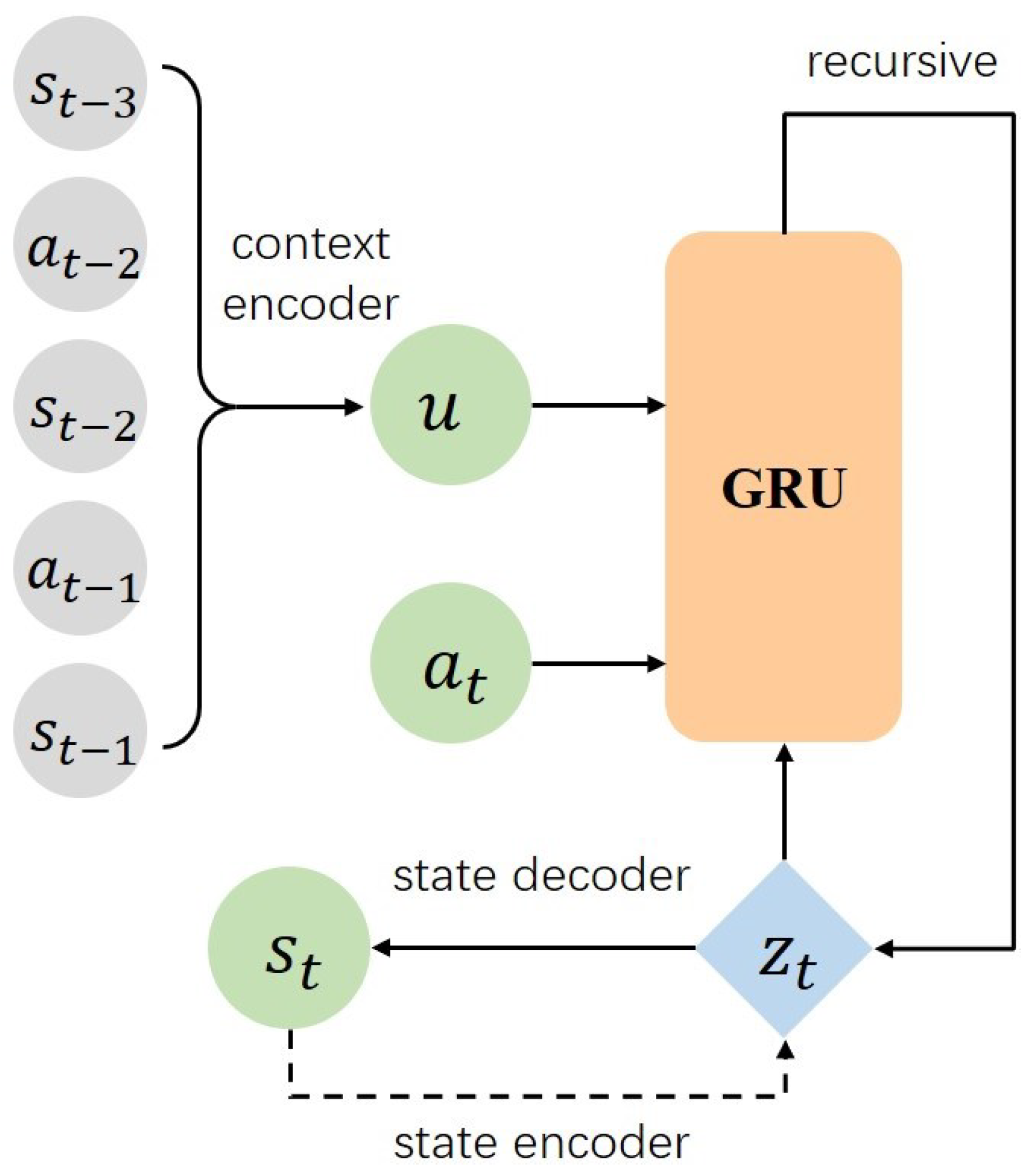
3.1. Decision-Time Learning with State Context Representation

We consider the state transition of the system to be generated by the following parametric MDP model:
s t + 1 = d s t ,   a t   , o + ϵ t
where s t S ,   a t A , and ϵ t N 0 ,   Q t . Here, Q t is the diagonal covariance matrix and o represents unobserved system parameters that actually influence the system state. The process can be treated as a Partially Observable Markov Decision Process (POMDP) [21]. We define T = ( s t ,   a t ,   s t + 1 ,   , a t + T 1 ,   s t + T ) as trajectory segments of length T, and C = s ,   a ,   s + as a set of system state representations, where s + = d ( s ,   a ,   o ) + ϵ . The objective of model learning is to determine a probabilistic context representation model d f s t ) s 0 : t 1 ,   a 0 : t 1 ,   C , which maximizes the expected log-likelihood function:
max θ E log p θ ( T C )
where θ denotes the parameters of the neural network. As we cannot directly observe o, we introduce a latent variable u to encode the context representation through learning:
log p θ ( T C ) = log p θ ( T u ) p θ ( u C ) d u
We use a neural network model d f s ^ t + H s ^ t ,   a t : t + H 1 ,   u to model p θ ( T u ) and apply a context representation encoder d c ( u C ) to model p θ ( u C ) . We construct an encoder to process the input sequence. Given a series of states s 0 : T , actions a 0 : T 1 , and the latent context representation variable u, the likelihood estimation of the predictive model d f is as follows:
p θ ( T u ) t = 0 T d f s ^ t = s t s t · t = 1 T d f s ^ t t 1 = s t s t 1 ,   a t 1 ,   u · t = 2 T d f s ^ t 0 = s t s 0 ,   a 0 : t 1 ,   u
The three terms in the above equation correspond to state reconstruction, single-step prediction, and multi-step prediction likelihood functions, respectively. The transition model d f s ^ t + H s ^ t ,   a t : t + H 1 ,   u is computed using the following equation:
s ^ t + H = h s t ,   a t ,   ,   a t + H 1 ,   u + ϵ
where ϵ is additive Gaussian noise with a mean of zero.
A Recurrent Neural Network (RNN) is a neural network architecture specifically designed to process sequential data, that features parameter sharing along the time dimension [22]. We use Gated Recurrent Units (GRUs) as a special type of RNN to construct the latent environment model, where h s ,   h a , and h u encode the state s t , action a t , and latent context representation vector u into the RNN loop:
z t = h s s t z t + 1 = h GRU z t ,   h a a t ,   h u ( u )
where [ · ,   · ] denotes vector concatenation. The decoders h s , μ and h s , σ 2 map the hidden state representation to a probability distribution over the state space:
s ^ t + H N h s , μ z t + H ,   diag h s , σ 2 z t + H
The context representation encoder d c ( u C ) encodes C as a Gaussian prior distribution over the latent context representation vector:
d c ( u C ) = N u h u , μ z u ,   diag h u , σ 2 z u
The latent space of the context representation encoder is further regularized by constraining the latent variable vector u to follow a unit Gaussian prior N ( 0 ,   I ) and applying KL-divergence loss:
L KL ( C ) = KL d c ( u C = { } ) N ( 0 ,   I )
The architecture of the modeling approach is illustrated in Figure 4.

3.2. Model Output Optimization with Separated Uncertainties

Since the actual operation of MHBC exhibits stochastic characteristics, the environment model should be formulated as a stochastic dynamic system to accurately capture the inherent uncertainties within the process. The uncertainties normally include aleatoric uncertainty and epistemic uncertainty. Aleatoric uncertainty arises from the inherent randomness of the environment, reflecting the system’s intrinsic stochastic nature. Epistemic uncertainty, on the other hand, arises from a lack of information and an insufficient ability to generalize beyond observed data, particularly in regions where data is sparse.
The Probabilistic Ensembles with Trajectory Sampling (PETS) [23] algorithm is a prominent method for incorporating model uncertainty into outputs. PETS leverages ensemble models to quantify both types of uncertainty simultaneously. In this study, we separately express aleatoric uncertainty and epistemic uncertainty, and finally integrate them into the planning process.
We consider using a Bayesian Neural Network (BNN) to capture aleatoric uncertainty. BNNs are based on Bayesian statistics and are trained using prior distribution knowledge [24]. We integrate an α -divergence minimization method to effectively capture aleatoric uncertainty in the BNN function.
The state transition model defined in Equation (1) can be expressed as follows:
y t = f x t ; W + ϵ t
where x t is the system’s input value, y t is the output value, f ( · ; W ) represents the neural network function parameterized by weight matrix W , and ϵ t is an additive noise term.
To enhance the model’s ability to capture aleatoric uncertainty, we introduce input perturbation in the neural network:
y t = f x t ,   z t ; W + ϵ t
where z t N ( 0 ,   γ ) represents random perturbation drawn from a normal distribution. The role of z t is to capture aleatoric uncertainty in the network’s output. The neural network consists of L layers, where the l-th layer contains M l hidden units. The weight matrices W = W l l = 1 L include M l × M l 1 + 1 weight matrices, each containing an additional bias term.
Let X be a T × D matrix containing system input values x t , and Y be a T × K matrix containing system output values y t . The vector z represents a T-dimensional random variable, including random terms z 1 ,   ,   z T . The likelihood function is then defined as follows:
p ( Y W ,   z ,   X ) = t = 1 T p y t W ,   z ,   x t = t = 1 T k = 1 K N y t , k f x t ,   z t ; W ,   Σ
The output is influenced by the additive noise variable ϵ t N ( 0 ,   Σ ) with diagonal covariance matrix Σ . For each z , the prior distribution follows a Gaussian distribution: N ( 0 ,   γ ) . Similarly, each element of the weight matrix W also follows a Gaussian prior distribution:
p ( z ) = t = 1 T N z t 0 ,   γ , p ( W ) = l = 1 L i = 1 M l j = 1 M l 1 + 1 N w i j , l 0 ,   λ
where w i j , l is the i ,   j -th element in the matrix W l , and γ and λ are the variances of the respective prior distributions. According to Bayes theorem, the posterior probability distribution of the weights W and perturbations z is given by the following:
p ( W ,   z D ) = p ( Y W ,   z ,   X ) p ( W ) p ( z ) p ( Y X )
where D is the data formed by input value x t and output value y t . Given a new input vector x ˜ , we can use the predictive distribution p ( y ˜ x ˜ ,   D ) to predict y ˜ :
p ( y ˜ x ˜ ,   D ) = N ( y ˜ f ( x ˜ ,   z ˜ ; W ) ,   Σ ) N ( z ˜ 0 ,   1 ) d z ˜ p ( W ,   z D ) d W d z
We approximate the exact posterior distribution p ( W ,   z D ) using a factorized Gaussian distribution:
q ( W ,   z ) = l = 1 L i = 1 M l j = 1 M l 1 + 1 N w i j , l m i j , l w ,   n i j , l w t = 1 T N z t m t z ,   n t z
The parameters m i j , l w ,   n i j , l w and m t z ,   n t z are determined by minimizing the divergence between p ( W ,   z D ) and q. After approximating q, we substitute p ( W ,   z D ) with q and use the mean values from q to approximate the integral in Equation (15). We adjust the parameters by minimizing the α -divergence between p ( W ,   z D ) and q ( W ,   z ) in Equations (15) and (16):
D α [ p ( W ,   z D ) q ( W ,   z ) ] = 1 α ( α 1 ) 1 p ( W ,   z D ) α q ( W ,   z ) ( 1 α ) d W d z
The α -divergence here is used to adjust the difference between distributions, allowing us to replace the posterior distribution with an approximate distribution q, thereby achieving efficient prediction and parameter optimization. The parameter α controls the properties of q. When α 1 ,   q tends to fit the entire posterior distribution p. When α 0 ,   q tends to fit the local regions of p. Setting α = 0.5 balances these two tendencies. We use the ensemble method to estimate epistemic uncertainty. The core idea is to leverage multiple stochastic models to represent the inherent randomness of the environment. The differences between models, which are constructed in the same manner, reflect the uncertainty caused by insufficient knowledge. We consider using the bootstrap ensemble method. Assume we perform bootstrap ensemble learning with K models, where E ^ k represents the ensemble of estimated parameters, and f k t ,   E ^ k represents the estimate output of the k-th model. Based on the Mean Squared Error (MSE) to evaluate model approximation quality, we assign a computational weight w k for each model k, satisfying the constraint w k = 1 :
w k = 1 M S E k 1 M S E 1 + 1 M S E 2 + + 1 M S E K
where M S E k represents the Mean Squared Error (MSE) of the k-th model, calculated as follows:
M S E k = 1 t j = 1 t f k t j ,   E ^ k y t j 2
Thus, the ensemble model’s average output estimate is given by the following:
f ens ( t ) = k = 1 K w k f k t ,   E ^ k
Assuming that the output probability sequence follows a Gaussian distribution with a mean of f ens ( t ) , we can use a parametric bootstrap ensemble method to construct a 95 % confidence interval. Specifically, suppose the training sample size is T, with time points t 1 ,   ,   t T . To generate bootstrap samples, we draw random variables y k from a Gaussian distribution with a mean of f ens t j . For each bootstrap sample y 1 ,   ,   y t , we can refit each model, compute the weights, and obtain the final ensemble model prediction. By performing this procedure multiple times, we can determine the 2.5 % and 97.5 % quantiles, thereby constructing the 95 % confidence interval.

4. Control Planning

After completing system identification by learning the environment model, the subsequent step is to leverage the learned model for control planning. Decision-time planning offers distinct advantages, as it bypasses the need for pre-trained policies and directly utilizes the environment model for planning at decision-time. However, two primary challenges arise: first, the accuracy of the learned model deteriorates over multi-step rollouts, posing difficulties in ensuring reliable long-term planning. Second, when applied to complex systems, decision-time planning is often conducted from a local perspective, increasing the risk of convergence to suboptimal solutions rather than achieving a globally optimal policy. Addressing these challenges is crucial for enhancing the robustness and effectiveness of decision-time planning.

4.1. Decision-Time Planning with Model Predictive Control

Model Predictive Control (MPC) is an iterative, model-based control method [25]. We apply MPC for decision-time planning, where at each time step, an optimization problem is iteratively solved to obtain an optimal action sequence. The first control input of this sequence is applied to the system, and the process is repeated at the next time step using the system’s updated state. The optimization objective of decision-time planning based on model predictive control is defined as follows:
max a 0 , , a H 1 t = 0 H 1 R s t ,   a t
where s t ,   a t represents the state and control input at time step t ,   H denotes the prediction horizon, and R s t ,   a t is the reward function. The control input a t is constrained within the range a min a t a max , where a min and a max represent the lower and upper bounds of the control input, respectively. These constraints ensure that the mild hyperbaric chamber control valve operates within a permissible range. MPC adopts a receding horizon approach, allowing the controller to dynamically adapt to changing conditions and disturbances at decision time.
The control task is optimized by a sequence reward R s t ,   a ^ . Starting from state s t , we apply an action sequence a ^ to predict the future trajectory over a horizon H. The expected cumulative reward is defined as the sum of the expected rewards of all particles s within the planning horizon H along the trajectory:
R s t ,   a ^ = Δ t = 1 H 1 K k = 1 K R s ˜ t + Δ t k ,   a t + Δ t
For action selection, we employ the Cross-Entropy Method (CEM) [26] to optimize the action sequence a ^ for reward maximization. To account for uncertainty in decision-time planning, the planner must avoid unpredictable regions in the state space, reducing their likelihood of selection.
In the previous chapter, we designed methods to separately model aleatoric uncertainty and epistemic uncertainty for output optimization. Here, we incorporate different uncertainty and define negative feedback penalty of aleatoric uncertainty as follows:
R A s t ,   a ^ = w A · Δ t = 1 H 1 K k = 1 K Σ θ k s ˜ t ,   a t
where Σ θ k s ˜ t ,   a t represents the predicted covariance matrix at the next time step t + 1 . The term w A > 0 is a weighting coefficient, where higher uncertainty will result in lower reward. To guide the exploration, we define the positive feedback reward for epistemic uncertainty as follows:
R E s t ,   a ^ = w E · Δ t = 1 H Var μ θ k s ˜ t ,   a t + Var θ k s ˜ t ,   a t
where Var represents the variance across k = 1 ,   ,   K ensemble models, and w E > 0 is a weighting coefficient.
The overall process of the algorithm is presented in Algorithm 1:    
Algorithm 1: Decision-Time planning with model predictive control
Input: number of samples N; number of particles P; planning horizon H; initial standard deviation σ init ; model output weights w A ,   w E
  1:
   for  t = 1 to T do:
  2:
      Initialize the mean vector μ 0 as a zero vector with dimension of R d × h
  3:
      Initialize the standard deviation vector σ 0 as a constant vector of dimension R d × h , with an initial value σ init
  4:
      for  i = 1 to the number of iterations do:
  5:
         Sample N samples from CEM μ t i , Σ t i , where each sample consists of P particles samples p p = 1 P
  6:
         Compute the cost function of each particle: c ,   c A ,   c E
  7:
         Compute the total cost: c total = c + c A + c E
  8:
         Select the top K samples with the lowest total cost as the elite set
  9:
         Fit a Gaussian distribution to the elite set and update the parameters: μ t i + 1 ,   Σ t i + 1
 10:
      Execute the first action from the final elite sequence

4.2. Policy Strengthening with Value Network

To address the challenge of decision-time planning converging to a local optimum, methods such as MCTS have been successfully employed. For example, AlphaZero, which utilizes decision-time planning, significantly outperforms off-line training by integrating MCTS during the on-line playing phase. However, MCTS is only applicable to discrete control problems, whereas MHBC control is a continuous control problem. In continuous control settings, decision-time planning can be guided by principles of policy iteration and value iteration, similar to model-free reinforcement learning. From this perspective, the objective function of decision-time planning is redefined as follows:
max a 0 , , a H 1 t = 0 H 1 R s t ,   a t + Q s H
where Q s H represents the Return function, which denotes the expected cumulative reward of the system starting from state S H . One of the most advanced methods for optimization from the perspective of value iteration is Temporal-Difference Model Predictive Control (TD-MPC) [27]. TD-MPC integrates the value function from reinforcement learning to address the limitations of traditional MPC, particularly its tendency to converge to locally optimal solutions within a limited planning horizon. The value function captures the expected cumulative reward over the trajectory, extending beyond the immediate planning window. By incorporating the value function, TD-MPC mitigates the risk of suboptimal convergence and enhances the discovery of globally optimal solutions. We consider further extending the TD-MPC method by integrating model-based learning and online model-free reinforcement learning to optimize the distribution of trajectories in decision-time planning control.
Since model-based learning is more sample-efficient, we utilize historical operational data from the mild hyperbaric chamber to rapidly complete the initial training phase. In the early stages, decision-time planning primarily relies on outputs from model-based learning. As planning progresses and online data accumulates, value functions are learned through a temporal difference approach. These value functions serve two key roles: (1) Enhancing model-based planning policies by guiding decision-time planning. (2) Generating online policies aligned with model-free reinforcement learning.
The planning process is presented in Algorithm 2. The more optimal policy is selected between the model-based policy Π θ and the online policy π θ . During the early deployment phase, the system strongly favors the model-based policy, and as long-term operation progresses, the system gradually incorporates more online policy considerations. The selection between these two strategies is regulated by parameter β , which starts at 100 % when the control system is initially deployed and gradually decreases to 25 % in long-term operation. That is, the algorithm selects actions from Π θ with probability β and selects actions from π θ with probability 1 β , prioritizing actions with higher estimated values from π θ .    
Algorithm 2: Value network guided Decision-Time planning (VN-DTP)
Input: learned network parameters θ ; initial parameters μ 0 ,   σ 0 ; number of samples/strategy trajectories N ,   N π ; current state s t ; planning horizon H; data buffer B ; Model-based policy Π θ ; online policy π θ ; selection parameter β
  1:
   Initialize all parameters
  2:
   for each iteration j = 1 J  do:
  3:
      Sample N trajectories of length H from N μ j 1 ,   σ j 1 2 I
  4:
      Sample N π trajectories of length H using π θ ,   d θ
  5:
      for all N + N π trajectories a t ,   a t + 1 ,   ,   a t + H  do:
  6:
            for  t = 0 H 1  do:
  7:
                ϕ Γ = ϕ Γ + γ t R θ ( s t ,   a t )
  8:
                s t + 1 d θ ( s t ,   a t )
  9:
             ϕ Γ = ϕ Γ + γ H Q θ ( s H ,   a H )
 10:
       μ j = i = 1 k Ω i Γ i * i = 1 k Ω i ,   σ j = i = 1 k Ω i ( Γ i * μ j ) 2 i = 1 k Ω i
 11:
      Updating parameter β
 12:
      if random ( 0 ,   1 ) < β  then:
 13:
          a t Π θ ( · h θ ( s t ) )
 14:
      else:
 15:
          a t argmax a t { Π ( s t ) , π ( s t ) } Q θ ( s t ,   a t )
 16:
       s t + 1 = P ( · s t ,   a t )
 17:
       B B ( s t ,   a t ,   r t ,   s t + 1 )

5. Performance Evaluation

5.1. Environment Setup

Main specifications of the MHBC used in the experiment are listed in Table 1.
The system employs a Siemens 200-Smart embedded computer (Munich, Germany) as the primary unit responsible for acquiring sensor readings and valve status data. These collected data are subsequently transmitted to the host computer for further processing. Concurrently, the embedded computer also executes valve control instructions received from the host computer. The host computer is equipped with an Intel i5 9400F CPU (Santa Clara, CA, USA) and an Nvidia RTX 2080Ti GPU (Santa Clara, CA, USA). The training and inference processes are accelerated by leveraging the GPU. To protect the valves, control command execution is separated by at least 1 s. The control system computation takes roughly 670 ms per step, thereby adequately satisfying real-time operation.
The pressures related to the MHBC include four variables: chamber pressure, air storage tank pressure, oxygen source pressure, and vacuum source pressure. The chamber pressure is the average value of multiple pressure sensors located at different positions inside the chamber. The oxygen source pressure and vacuum source pressure are controlled by the configured values of the oxygen concentrator and vacuum pump, respectively. These two pressure values affect system states as action inputs in practice and are, therefore, categorized as action variables. The action variables in the MHBC control system also include: two pressurization control valves in the pressurization pipeline; two depressurization control valves in the depressurization pipeline; one oxygen supply control valve in the oxygen supply pipeline; and one oxygen exhaust control valve in the oxygen exhaust pipeline. As a result, the system consists of two state variables and eight action variables.

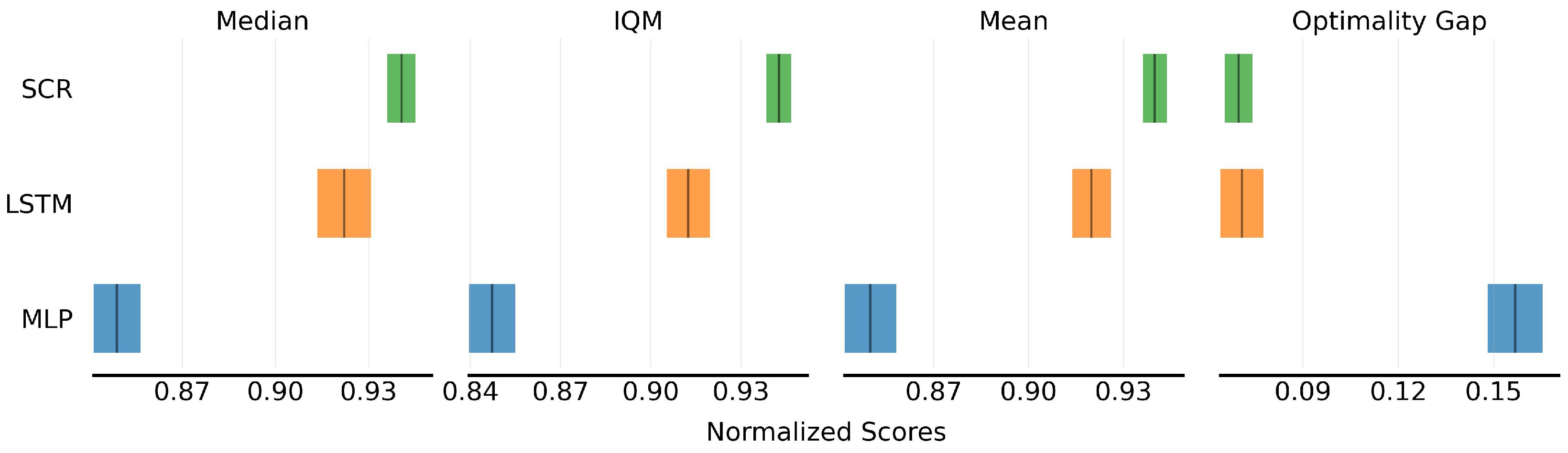
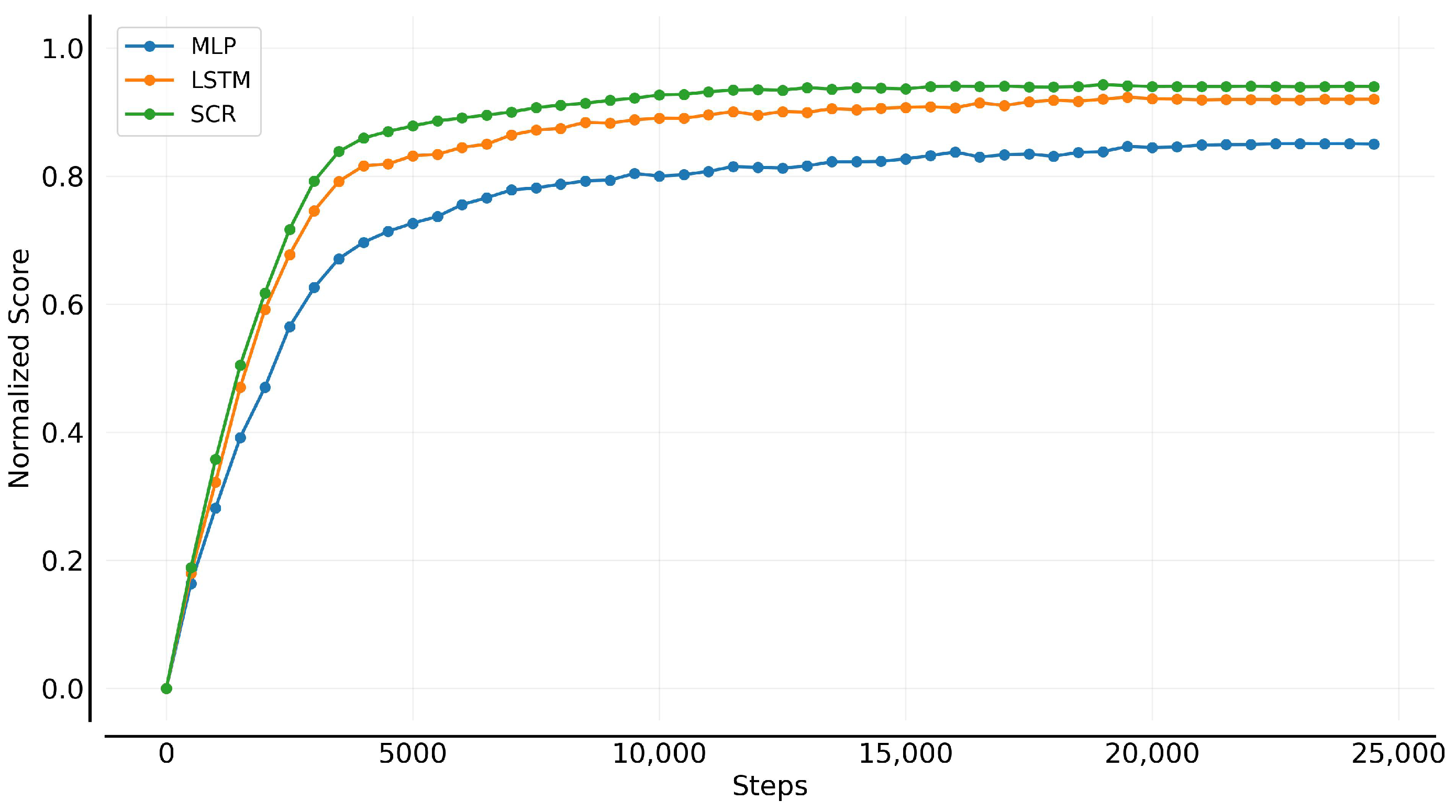
5.2. Model Learning Evaluation

First, we evaluate the effectiveness of state context representation learning in our model. Regarding the neural network architecture, we use Linear ( M ,   N ) to denote linear layer with M input features and N output features, ReLU ( ) to represent the rectified linear unit activation function, Tanh () to indicate the hyperbolic tangent activation function, and Softplus() to denote smoothed rectified linear unit activation function with additive bias. As described in Section 5.1, the system has a state dimension of D S = 2 , and an action dimension of D A = 8 . We define the latent state dimension in GRU as D Z = 20 , and a state context representation dimension as D C = 20 . The proposed neural network architecture is as follows:
State encoder:
Linear D S ,   50 ;   ReLU ( ) ;   Linear 50 ,   D Z ;   Tan h ( )
State decoder:
Linear D Z ,   50 ;   ReLU ( ) ;   Linear 50 ,   D S
Action encoder for GRU:
Linear D A ,   50 ;   ReLU ( ) ;   Linear 50 ,   D Z ;   ReLU ( )
Context representation transformation from the past three states and actions information:
Linear 3 × D S + D A ,   50 ;   ReLU ( ) ;   Linear 50 ,   D C ;   ReLU ( )
Context representation encoder for GRU:
Linear D C ,   50 ;   ReLU ( ) ;   Linear 50 ,   D Z ;   ReLU ( )
We focus on algorithm research rather than investigating variations in the internal structure of neural networks. Therefore, the basic neural network structure remains unchanged across different algorithmic comparisons. The architectures of the Multilayer Perceptron (MLP) network and Long Short-Term Memory (LSTM) network used for comparison are as follows:
MLP:
[ Linear ( D S + D A ,   50 ) ;   ReLU ( ) ;   Linear ( 50 ,   D Z ) ;   ReLU ( ) ;   Linear ( D Z ,   50 ) ;
ReLU ( ) ;   Linear ( 50 ,   D S ) ]
Input and Output of the LSTM:
[ Linear ( D S + D A ,   50 ) ;   ReLU ( ) ;   Linear ( 50 ,   D Z ) ;   ReLU ( ) ;   Linear ( D Z ,   50 ) ;
ReLU ( ) ;   Linear ( 50 ,   D S ) ]
Recursion of the LSTM:
Linear D Z ,   50 ;   ReLU ( ) ;   Linear 50 ,   D Z
Under these neural network architectures, we compare our proposed state context representation (denoted as SCR) method with models learned using MLP and LSTM. The evaluation is conducted on average score and sample efficiency [28]. For the average score, we assess the performance using the following four metrics: (1) Median: The middle value of the performance scores across multiple runs. (2) Interquartile Mean (IQM): The mean score calculated after discarding the lowest 25 % and highest 25 % of results, retaining only the middle 50 % . (3) Mean: The arithmetic average of all performance scores. (4) Optimality Gap: The difference between the algorithm’s performance and the predefined optimal performance threshold. The optimal performance threshold is established based on a predefined criterion for satisfactory control performance, beyond which further improvements yield diminishing effects. Specifically, we define this threshold as pressure control error below 5 Pa. For sample efficiency, we analyze how the objective function value changes during the training process, providing insights into the algorithm’s data requirements.
Figure 5 presents the average scores with 95 % Confidence Interval (CI) of different model predictions. From the metrics, it can be observed that after incorporating LSTM and SCR, the average score of the algorithms are improved by approximately 6.8 % and 9.2 % , respectively, compared to MLP. This improvement is attributed to the ability of recursive structures to capture long-term dependencies in temporal sequences. By effectively retaining hidden state information in partially observable Markov decision processes, these methods enable the model to make more accurate inferences about the current state based on historical observations. The proposed SCR learning approach further enhances the model’s understanding of complex environmental dynamics by extracting intrinsic information and achieves further improvements over LSTM.
Figure 6 illustrates the asymptotic and convergence performance of different environment model architectures. The experimental results indicate that the LSTM and SCR significantly outperform the MLP-based approach in terms of data efficiency and stability. In contrast, the MLP-based approach exhibits a relatively slower convergence rate during training and shows greater fluctuations, suggesting certain limitations in learning complex dynamic environments.
Next, we evaluate the effectiveness of model output optimization from two perspectives: average score and performance profile. For performance profile, we analyze the distribution of scores, which provides insights into the distribution of the algorithm’s performance. We compare four algorithms: (1) RS (Random Shooting): the random shooting search method; (2) CEM (Cross-Entropy Method): standard cross-entropy-based approach; (3) PETS (Probabilistic Ensemble and Trajectory Sampling): CEM method that integrates PETS; amd (4) CEM-SEP (Cross-Entropy Method with separated uncertainty measurement): our proposed method, which separately quantifies epistemic uncertainty and aleatoric uncertainty. The control system operates based on the designed decision-time planning with model predictive control.
Figure 7 compares the performance of the algorithms in model output optimization. In planning score metrics, CEM outperforms RS by approximately 6.1 % . RS relies on uniform random sampling across the entire action space, which struggles to identify optimal policies in complex dynamic environments. In contrast, CEM utilizes an adaptive probability distribution update mechanism to iteratively converge toward high-quality actions, thereby improving decision efficiency. With the introduction of probabilistic ensemble and trajectory sampling, control precision further improves by approximately 4.3 % . PETS enhances model prediction accuracy by training multiple environment models and estimating uncertainty during trajectory sampling. By separately modeling aleatoric and epistemic uncertainty, and then combining both for joint modeling, the CEM-SEP algorithm achieves a 1.2% performance increase compared to the PETS algorithm.
Figure 8 compares the performance distribution of different output optimization methods as the fractions of scores that are greater than its normalized average score. It can be observed that the CEM method, by adaptively adjusting the sampling distribution, more effectively converges to high-quality action sequences compared to the RS method. Building upon the CEM method, further optimization of model output uncertainty results in PETS and CEM-SEP achieving more desirable output distributions.

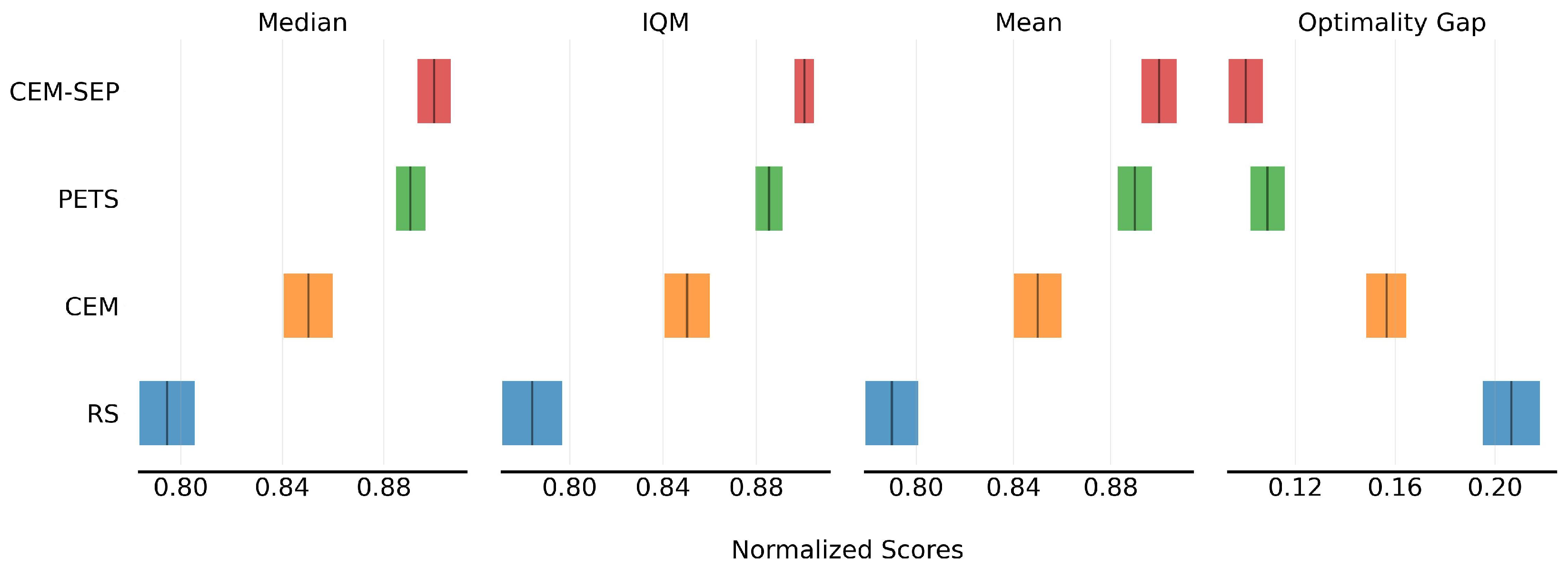
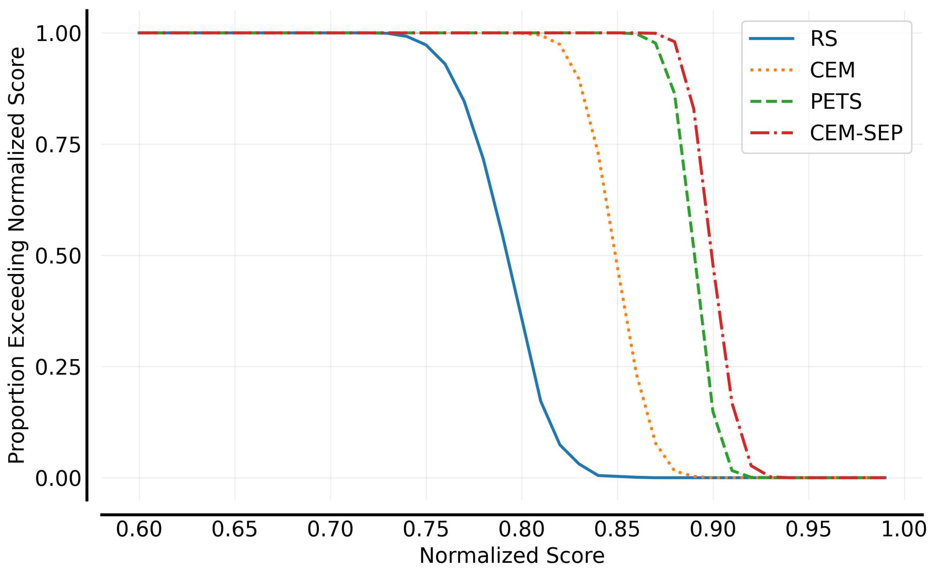
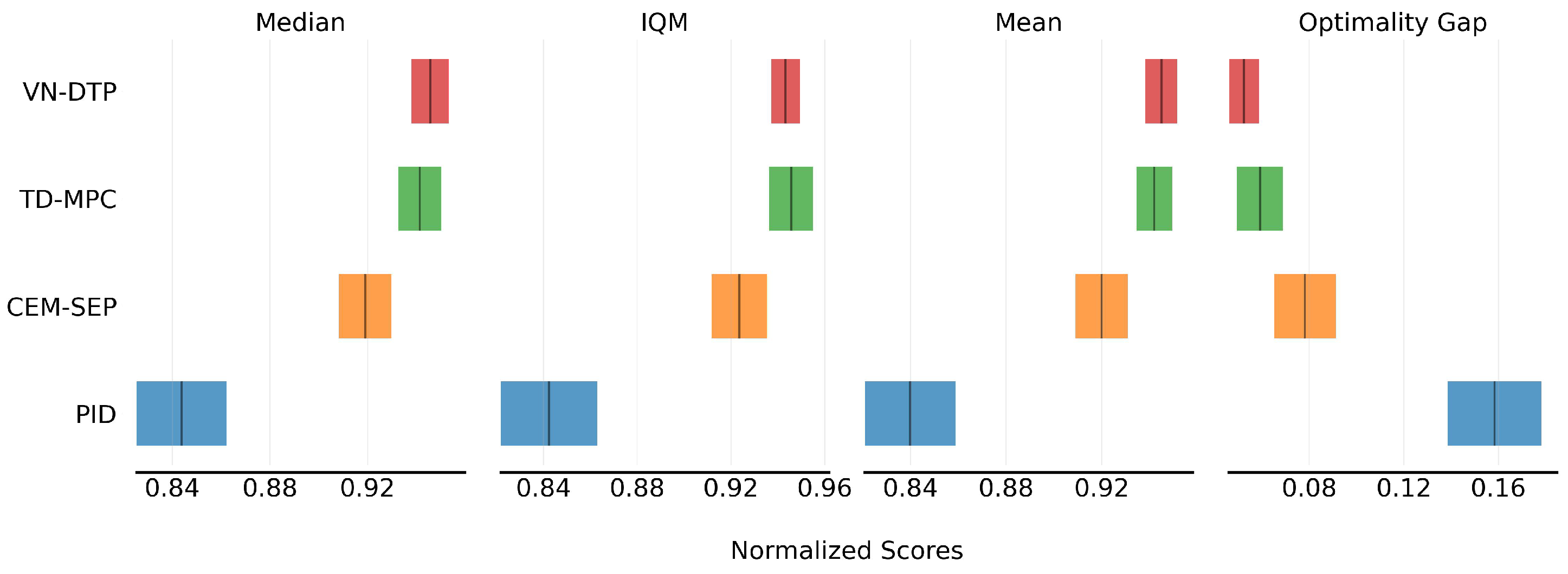
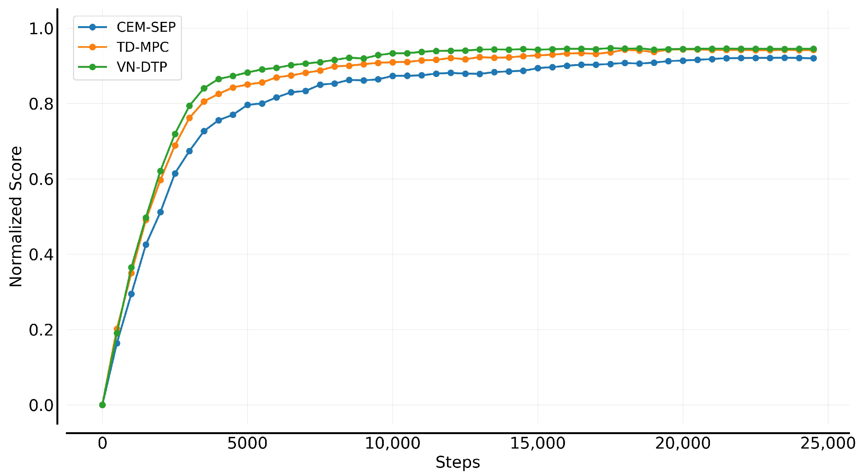
5.3. Control Planning Evaluation

We evaluate the control planning results by comparing the algorithms in terms of average score and sample efficiency. The compared algorithms include: (1) PID: the proportional-integral-derivative control algorithm; (2) CEM-SEP: model-based decision-time planning algorithm using cross-entropy method with separated uncertainty measurement; (3) TD-MPC: extension of CEM-SEP with temporal difference model predictive control; and (4) VN-DTP (Value Network guided Decision-Time Planning): our further proposed approach that utilizes value network and online policy to guide decision-time planning.
The hyperparameter settings of are summarized in Table 2.
Figure 9 presents the average scores of the algorithms. From the metrics, it is evident that applying decision-time planning algorithms results in significant performance improvements compared to the PID control algorithm. Specifically, CEM-SEP outperforms PID by approximately 7.8%. TD-MPC further improves upon CEM-SEP by an additional 2.3% through the incorporation of a value network, which enhances modeling of long-term returns and facilitates better trade-offs between short-term and long-term rewards. VN-DTP achieves the best performance, surpassing TD-MPC by a further 0.4%, attributed to its integration of an online policy during planning. Ultimately, VN-DTP achieved a performance improvement exceeding 10.5% compared to the commercial PID algorithm applied in MHBC.
Figure 10 compares the asymptotic and convergence performance of different decision-time planning algorithms. It can be observed that, compared to the baseline CEM-SEP planning algorithm, incorporating value networks leads to significant improvements in both progression and convergence. The VN-DTP algorithm exhibits a notably faster asymptotic rate within the first 4000 timesteps, followed by a steady convergence in the later stages of training.
We also design experiments to evaluate the algorithm’s performance when the system is facing abnormal conditions. We consider three types of abnormal scenarios:
  • Valve calibration offset: Simulated by introducing small random disturbances into the valve calibration values.
  • Valve failure: Simulated by either setting the valve completely closed or fixing it at a specific opening, with the valve potentially reporting correct or incorrect feedback to the control system.
  • Chamber leakage: Simulated by introducing unexpected additional valve openings.
More specifically, the above abnormal conditions are categorized into the following six scenarios:
  • Valve calibration offset: Originally, the valve opens at a set-point of 5%; due to prolonged usage, it now opens only when the input reaches 6%.
  • Valve permanently closed with correct feedback: Valve remains fully closed regardless of inputs, correctly reporting this closed status.
  • Valve permanently closed with incorrect feedback: Valve remains fully closed regardless of inputs, incorrectly reporting it as open at the commanded position.
  • Valve stuck at fixed opening with correct feedback: Valve remains open at a random fixed opening (2–10%), correctly reporting this actual fixed opening.
  • Valve stuck at fixed opening with incorrect feedback: Valve remains open at a random fixed opening (2–10%), incorrectly reporting it as open at the commanded position.
  • Simulated chamber leakage: Valve maintains a baseline opening of 1–5%, with additional commanded openings added on top, simulating a chamber leak.
Table 3 presents the average score of the algorithms under these abnormal conditions. It can be observed that the PID algorithm experiences a significant performance degradation of about 11.8 % compared to normal conditions in Figure 9. In contrast, the impact of valve failures on CEM-SEP, TD-MPC, and VN-DTP is relatively minor, with performance drops of 10.8 % , 8.3 % , and 7.7 % , respectively, as these model-based algorithms incorporate state context representation within their dynamic models, enabling certain adaptability to system abnormalities.

6. Concluding Remarks

This paper tackles the challenges of data efficiency and non-stationary dynamics in MHBC control by proposing a decision-time learning and planning integrated framework. The framework consists of: (1) decision-time model learning based on state context representation; (2) model output optimization for separated uncertainties; (3) decision-time planning with model predictive control; and (4) trajectory optimization through value network and online policy guidance. Experimental results demonstrate the effectiveness of the proposed algorithms.
As a type of Pressure Vessel for Human Occupancy (PVHO), MHBC shares similarities with diving decompression chambers, tunnel boring machine pressure chambers, hypobaric chambers, and other pressure chambers. The proposed algorithm utilizes historical operational data from an existing system to learn an optimized control policy. By leveraging this data-driven approach, the algorithm can achieve competitive performance as soon as it is deployed on a real-world system, making it applicable to other similar PVHO control systems.
Future research could further explore hybrid architectures incorporating safety shields, control barrier functions, or safe reinforcement learning to enhance system reliability in safety-critical medical applications. Additionally, integrating interpretability tools such as feature attribution, saliency maps, or uncertainty visualization could improve the transparency and trustworthiness of model decisions.

Author Contributions

Conceptualization, N.Z.; methodology, N.Z.; software, N.Z.; validation, N.Z. and Q.L.; formal analysis, N.Z.; investigation, N.Z.; resources, Z.J.; data curation, N.Z.; writing—original draft preparation, N.Z.; writing—review and editing, N.Z. and Q.L.; visualization, N.Z.; supervision, Z.J.; project administration, Z.J. All authors have read and agreed to the published version of the manuscript.

Funding

This research received no external funding.

Data Availability Statement

Dataset available on request from the authors.

Conflicts of Interest

The authors declare no conflicts of interest.

References

  1. Ortega, M.A.; Fraile-Martinez, O.; García-Montero, C.; Callejón-Peláez, E.; Sáez, M.A.; Álvarez-Mon, M.A.; García-Honduvilla, N.; Monserrat, J.; Álvarez-Mon, M.; Bujan, J.; et al. A general overview on the hyperbaric oxygen therapy: Applications, mechanisms and translational opportunities. Medicina 2021, 57, 864. [Google Scholar] [CrossRef] [PubMed]
  2. Lefebvre, J.C.; Lyazidi, A.; Parceiro, M.; Sferrazza Papa, G.F.; Akoumianaki, E.; Pugin, D.; Tassaux, D.; Brochard, L.; Richard, J.C.M. Bench testing of a new hyperbaric chamber ventilator at different atmospheric pressures. Intensive Care Med. 2012, 38, 1400–1404. [Google Scholar] [CrossRef] [PubMed]
  3. de Paco, J.M.; Pérez-Vidal, C.; Salinas, A.; Gutiérrez, M.D.; Sabater, J.M.; Fernández, E. Advanced hyperbaric oxygen therapies in automated multiplace chambers. In Proceedings of the 2012 4th IEEE RAS & EMBS International Conference on Biomedical Robotics and Biomechatronics (BioRob), Rome, Italy, 24–27 June 2012; IEEE: Piscataway, NJ, USA, 2012; pp. 201–206. [Google Scholar]
  4. Wang, B.; Wang, S.; Yu, M.; Cao, Z.; Yang, J. Design of atmospheric hypoxic chamber based on fuzzy adaptive control. In Proceedings of the 2013 IEEE 11th International Conference on Electronic Measurement & Instruments, Harbin, China, 16–19 August 2013; IEEE: Piscataway, NJ, USA, 2013; Volume 2, pp. 943–946. [Google Scholar]
  5. Gracia, L.; Perez-Vidal, C.; de Paco, J.M.; de Paco, L.M. Identification and control of a multiplace hyperbaric chamber. PLoS ONE 2018, 13, e0200407. [Google Scholar] [CrossRef] [PubMed]
  6. Motorga, R.M.; Muresan, V.; Abrudean, M.; Valean, H.; Clitan, I.; Chifor, L.; Unguresan, M. Advanced Control of Pressure Inside a Surgical Chamber Using AI Methods. In Proceedings of the 2023 3rd International Conference on Electrical, Computer, Communications and Mechatronics Engineering (ICECCME), Tenerife, Canary Islands, Spain, 19–21 July 2023; IEEE: Piscataway, NJ, USA, 2023; pp. 1–8. [Google Scholar]
  7. Ladosz, P.; Weng, L.; Kim, M.; Oh, H. Exploration in deep reinforcement learning: A survey. Inf. Fusion 2022, 85, 1–22. [Google Scholar] [CrossRef]
  8. Silver, D.; Schrittwieser, J.; Simonyan, K.; Antonoglou, I.; Huang, A.; Guez, A.; Hubert, T.; Baker, L.; Lai, M.; Bolton, A.; et al. Mastering the game of go without human knowledge. Nature 2017, 550, 354–359. [Google Scholar] [CrossRef] [PubMed]
  9. Wu, T.; He, S.; Liu, J.; Sun, S.; Liu, K.; Han, Q.L.; Tang, Y. A brief overview of ChatGPT: The history, status quo and potential future development. IEEE/CAA J. Autom. Sin. 2023, 10, 1122–1136. [Google Scholar] [CrossRef]
  10. Tutsoy, O.; Asadi, D.; Ahmadi, K.; Nabavi-Chashmi, S.Y.; Iqbal, J. Minimum distance and minimum time optimal path planning with bioinspired machine learning algorithms for faulty unmanned air vehicles. IEEE Trans. Intell. Transp. Syst. 2024, 25, 9069–9077. [Google Scholar] [CrossRef]
  11. Afifa, R.; Ali, S.; Pervaiz, M.; Iqbal, J. Adaptive backstepping integral sliding mode control of a mimo separately excited DC motor. Robotics 2023, 12, 105. [Google Scholar] [CrossRef]
  12. Baillieul, J.; Samad, T. Encyclopedia of Systems and Control; Springer: Cham, Switzerland, 2021. [Google Scholar]
  13. Borase, R.P.; Maghade, D.; Sondkar, S.; Pawar, S. A review of PID control, tuning methods and applications. Int. J. Dyn. Control 2021, 9, 818–827. [Google Scholar] [CrossRef]
  14. Luo, F.M.; Xu, T.; Lai, H.; Chen, X.H.; Zhang, W.; Yu, Y. A survey on model-based reinforcement learning. Sci. China Inf. Sci. 2024, 67, 121101. [Google Scholar] [CrossRef]
  15. Sutton, R.S.; Barto, A.G. Reinforcement Learning: An Introduction. A Bradford Book; The MIT Press: Cambridge, MA, USA, 2018. [Google Scholar]
  16. Janner, M.; Fu, J.; Zhang, M.; Levine, S. When to trust your model: Model-based policy optimization. In Advances in Neural Information Processing Systems, Proceedings of the 33rd Conference on Neural Information Processing Systems (NeurIPS 2019), Vancouver, BC, Canada, 8–14 December 2019; Curran Associates Inc.: Red Hook, NY, USA, 2019; Volume 32. [Google Scholar]
  17. Levine, S.; Abbeel, P. Learning neural network policies with guided policy search under unknown dynamics. In Advances in Neural Information Processing Systems, Proceedings of the 28th International Conference on Neural Information Processing Systems, Montréal, QC, Canada, 8–13 December 2014; MIT Press: Cambridge, MA, USA, 2014; Volume 27. [Google Scholar]
  18. Deisenroth, M.; Rasmussen, C.E. PILCO: A model-based and data-efficient approach to policy search. In Proceedings of the 28th International Conference on Machine Learning (ICML-11), Bellevue, WA, USA, 28 June–2 July 2011; pp. 465–472. [Google Scholar]
  19. Kahneman, D. A perspective on judgment and choice: Mapping bounded rationality. In Progress in Psychological Science Around the World. Volume 1 Neural, Cognitive and Developmental Issues; Psychology Press: Hove, UK, 2013; pp. 1–47. [Google Scholar]
  20. Altman, E. Constrained Markov Decision Processes; Routledge: London, UK, 2021. [Google Scholar]
  21. Kurniawati, H. Partially observable markov decision processes and robotics. Annu. Rev. Control Robot. Auton. Syst. 2022, 5, 253–277. [Google Scholar] [CrossRef]
  22. Bonassi, F.; Farina, M.; Scattolini, R. On the stability properties of gated recurrent units neural networks. Syst. Control Lett. 2021, 157, 105049. [Google Scholar] [CrossRef]
  23. Chua, K.; Calandra, R.; McAllister, R.; Levine, S. Deep reinforcement learning in a handful of trials using probabilistic dynamics models. In Advances in Neural Information Processing Systems, Proceedings of the 32nd International Conference on Neural Information Processing Systems, Montréal, QC, Canada, 3–8 December 2018; Curran Associates Inc.: Red Hook, NY, USA, 2018; Volume 31. [Google Scholar]
  24. Izmailov, P.; Vikram, S.; Hoffman, M.D.; Wilson, A.G.G. What are Bayesian neural network posteriors really like? In Proceedings of the International Conference on Machine Learning, PMLR, Virtual, 18–24 July 2021; pp. 4629–4640. [Google Scholar]
  25. Hewing, L.; Wabersich, K.P.; Menner, M.; Zeilinger, M.N. Learning-based model predictive control: Toward safe learning in control. Annu. Rev. Control. Robot. Auton. Syst. 2020, 3, 269–296. [Google Scholar] [CrossRef]
  26. Zhang, Z.; Jin, J.; Jagersand, M.; Luo, J.; Schuurmans, D. A simple decentralized cross-entropy method. In Advances in Neural Information Processing Systems, Proceedings of the 36th International Conference on Neural Information Processing Systems, New Orleans, LA, USA, 28 November–9 December 2022; Curran Associates Inc.: Red Hook, NY, USA, 2022; Volume 35, pp. 36495–36506. [Google Scholar]
  27. Hansen, N.; Wang, X.; Su, H. Temporal difference learning for model predictive control. arXiv 2022, arXiv:2203.04955. [Google Scholar]
  28. Agarwal, R.; Schwarzer, M.; Castro, P.S.; Courville, A.C.; Bellemare, M. Deep reinforcement learning at the edge of the statistical precipice. In Advances in Neural Information Processing Systems, Proceedings of the 35th International Conference on Neural Information Processing Systems, Online, 6–14 December 2021; Curran Associates Inc.: Red Hook, NY, USA, 2021; Volume 34, pp. 29304–29320. [Google Scholar]
Figure 1. Vehicle-mounted plateau MHBC.
Algorithms 18 00380 g001
Figure 2. Layout diagram of the MHBC.
Algorithms 18 00380 g002
Figure 3. Pipeline diagram of the MHBC.
Algorithms 18 00380 g003
Figure 4. The proposed state context representation model.
Algorithms 18 00380 g004
Figure 5. SCR outperforms other methods in average score with 95 % CI of model prediction.
Algorithms 18 00380 g005
Figure 6. Asymptotic and convergence performance of model prediction.
Algorithms 18 00380 g006
Figure 7. CEM-SEP outperforms other methods in average score with 95% CI of different model outputs.
Algorithms 18 00380 g007
Figure 8. Performance profile of different model outputs.
Algorithms 18 00380 g008
Figure 9. VN-DTP outperforms other methods in average score with 95% CI of different control algorithms.
Algorithms 18 00380 g009
Figure 10. Asymptotic and convergence performance of different control methods.
Algorithms 18 00380 g010
Table 1. Main specifications of the mild hyperbaric chamber.
Technical SpecificationMHBC
Total chamber volume 12.4   m 3
Design pressure0.155 MPa
Maximum operating pressure0.150 MPa
Cabin temperatureWinter: 20 ± 2   ° C Summer: 24 ± 2   ° C
Cabin humidity40–50%
Standard capacity4 persons
Pressurization rate 0.004 0.015   MPa / min
Depressurization rate 0.004 0.01   MPa / min
Oxygen concentration inside21–23%
Air supply pressure0.5 MPa
Air storage tank capacity 3   m 3
Air compressor output rate 0.9   m 3 / min
Table 2. Hyperparameter settings for TD-MPC and VN-DTP.
HyperparameterValue
Discount factor ( γ ) 0.99
Initial steps10
Planning horizon30
Initial parameters ( μ 0 ,   σ 0 ) (0, 2)
Population size128
Elite ratio16
Iterations6
Shrink ratio5%
Number of particles1
Momentum coefficient0.1
Learning rate3 × 10−4
Optimizer ( θ ) Adam ( β 1 = 0.9 ,   β 2 = 0.999 )
Temporal coefficient ( λ ) 0.5
Exploration rate ( ϵ ) 0.5 → 0.05
Planning horizon scheduling 1 5
Batch size128
Momentum coefficient0.99
Gradient updates per step1
θ update frequency2
Table 3. Cumulative score comparison in fault-tolerant control under six cases.
AlgorithmCaseAverage
123456
PID0.7480.7340.6930.7260.7050.7260.722
CEM-SEP0.8390.8230.7850.8160.7970.8120.812
TD-MPC0.8720.8610.8410.8620.8530.8670.859
VN-DTP0.8800.8690.8520.8730.8620.8730.868
Disclaimer/Publisher’s Note: The statements, opinions and data contained in all publications are solely those of the individual author(s) and contributor(s) and not of MDPI and/or the editor(s). MDPI and/or the editor(s) disclaim responsibility for any injury to people or property resulting from any ideas, methods, instructions or products referred to in the content.

