Abstract
The circadian rhythm plays a crucial role in regulating biological processes, and its disruption is linked to various health issues. Identifying small molecules that influence the circadian period is essential for developing targeted therapies. This study explores the use of evolutionary optimization techniques to enhance the classification of these molecules. We applied a genetic algorithm to optimize feature selection and classification performance. Several tree-based learning classification algorithms (Decision Trees, Extra Trees, Random Forest, XGBoost) and a distance-based classifier (kNN) were employed. Their performance was evaluated using accuracy and F1-score, while considering their generalization ability with a validation set. The findings demonstrate that the proposed genetic algorithm improves classification accuracy and reduces overfitting compared to baseline models. Additionally, the use of variance in accuracy as a penalty factor may enhance the model’s reliability for real-world applications. Our study confirms that evolutionary optimization is an effective strategy for classifying small molecules regulating the circadian rhythm. The proposed approach not only improves predictive performance but also ensures a more robust model.
1. Introduction
The circadian rhythm regulates biological processes in 24 h cycles, and its alteration is associated with sleep disorders and can be related to pathologies such as cancer [1]. The circadian clock plays a fundamental role in the regulation of sleep, and its stability is increasingly recognized as a determining factor in various biological processes, which are essential for maintaining good health. To this end, photopharmacological manipulation of a core clock protein, mammalian Cryptochrome 1 (CRY1), is an effective strategy for the regulation of the circadian clock. CRY1 is a protein that influences the circadian period. Supported by the analysis of data and advanced computational modelling techniques, it has been established as an essential tool in the detection and characterization of compounds with an impact on circadian dynamics [2]. Recent studies have applied high-throughput screening and data analysis to identify potential drugs, taking advantage of advanced modelling and machine learning techniques [3].
Structural approaches in drug discovery optimize efficiency and reduce costs, while the incorporation of screening methods allows the elimination of inappropriate molecules, such as toxic or inactive ones. After identifying 171 molecules that target functional domains of the CRY1 protein, using structure-based drug design methods, and experimentally determining that 115 of these molecules were nontoxic, Gul et al. [4] performed a machine learning study to classify molecules by identifying features that make them toxic. They also addressed the classification of the same molecules based on their effect on CRY1. While both problems are considered challenging, only the second has been further investigated in other studies [5].
The problem of learning to determine toxicity from these 171 molecules is complex, characterized by many features and few examples. As a result, it is considered ill-posed, as traditional statistical methods often struggle with insufficient data. In this context, overfitting becomes a significant risk, as models can easily memorize the training data instead of generalizing. Therefore, we classify it as an overfitting-prone problem. Tackling these handicaps constitutes an interesting challenge in machine learning [6]. These handicaps motivate us to apply improved automated feature selection while remaining fully aware of its limitations.
In this paper, we reproduce the machine learning experimentation from [4], revealing its weaknesses and evaluating the use of a more advanced feature selection process based on genetic algorithm meta-heuristic search to achieve improved and more trustworthy results.
The main contributions of this paper are as follows:
- Demonstration of the need for validation: We make evident the importance of incorporating validation after training and feature selection to avoid overfitting. In addition, we provide reliable estimates of the best performance achieved with this dataset.
- Genetic algorithm for automated feature selection: We propose a genetic algorithm (GA)-based framework for automated feature selection, which achieves results comparable to or better than manual Recursive Feature Elimination (RFE), reducing human effort and bias.
- Test variance as a generalization criterion: We propose the use of variance across cross-validation folds as an additional objective during feature selection, promoting models that not only perform well but also generalize better across different data splits.
2. Genetic Algorithm for Feature Selection
Evolutionary algorithms, inspired by natural evolution, are designed to optimize solutions. Among them, genetic algorithms (GAs) are particularly well-suited for feature selection (FS). These algorithms start with a population of individuals, each representing a possible solution. Through processes of selection, crossover, and mutation, successive generations evolve towards better solutions, until the number of generations specified by parameter N is reached (Figure 1). The following subsections describe the main aspects of the algorithm used in this work.
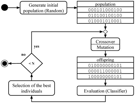
Figure 1.
Genetic algorithm activity diagram.
2.1. Evolution
The framework of the algorithm is based on the evolution of a single population of solutions over multiple generations.
Once the population has been initialized, each evolutionary cycle begins with the application of crossover and mutation operators to generate new solutions. Subsequently, the individuals in the population are evaluated and selected, based on their performance in the target task, to form the next generation with the objective of progressively improving the quality of the solutions. Figure 1 illustrates the main steps of the algorithm.
2.2. Encoding
The encoding of solutions determines how potential solutions to the problem are represented. Each solution is encoded as a genotype, which serves as an abstract representation of the solution. To evaluate its quality, the genotype is decoded into its corresponding phenotype, representing the actual interpretation within the problem domain. The effectiveness of the encoding scheme directly influences the algorithm’s ability to explore and optimize solutions efficiently.
In this work, the chosen encoding scheme is binary. Each individual in the population represents a possible solution to the problem, which is described as a vector of length n. Each value in the vector corresponds to a feature of the problem, with a 1 indicating that the feature is selected and a 0 otherwise.
2.3. Initialization
In an evolutionary algorithm, the initial population is generated randomly, assigning to each individual an initial configuration that represents a possible solution to the problem. However, the nature of the problem significantly influences the optimal configuration of individuals. Depending on the dimensionality of the dataset and the complexity of the problem, the expected number of selected features may vary considerably.
GAs typically initialize individuals with a uniform probability of inclusion or exclusion of each feature, resulting in an expected selection of 50% of the features. However, in high-dimensionality datasets, this strategy can generate overfitted initial solutions, which significantly slows down the evaluation of individuals. Since the GA will naturally adjust the number of features selected based on their impact on performance, a more efficient initialization strategy may be to start with a smaller number of features when working with high-dimensional spaces [7].
To strike a balance between simplicity and generality, the initialization strategy used in our algorithm is based on an adjustable likelihood as parameter [8].
2.4. Crossover Operator
The crossover operation combines coded individuals to explore potentially better solutions. In this work, two-point crossover, a method widely used in GAs, is employed to generate the next generation within the population. This mechanism exchanges a segment of the genotypic vector between two parent individuals, bounded by two randomly selected points. Figure 2 illustrates this process. The probability of selecting segments of different sizes and their location within the genotype is uniform, ensuring a balanced exploration of the search space without introducing biases in the optimization.
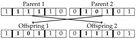
Figure 2.
Crossover operator.
2.5. Mutation Operator
The mutation operation on encoded individuals introduces random modifications in the population to preserve genetic diversity. This mechanism is crucial for preventing premature convergence, allowing the algorithm to explore a broader search space and reducing the risk of getting trapped in local optima. In this study, the bit-flip mutation operator is employed, a widely used technique in binary-encoded GAs. This operator selectively alters certain binary values within the genotype of each individual, flipping them with a predefined probability, which serves as a control parameter for the mutation intensity. Figure 3 illustrates this process.
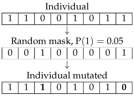
Figure 3.
Mutation operator.
2.6. Fitness Evaluation
Fitness evaluation in a GA is the process of assessing how well each individual in the population solves the given problem. The fitness function quantitatively measures the quality of each solution based on a predefined criterion. In the case of feature selection problems, this criterion is the efficiency of the selected feature subset. The fitness score determines the likelihood of an individual being selected for reproduction, guiding the evolutionary process toward optimal solutions over successive generations.
In this work, we use the wrapper approach with 10-fold cross-validation to evaluate the quality of each individual (feature subset). The fitness of an individual is determined by training a machine learning model using the selected features, represented by the genotype, and evaluating its performance based on the accuracy metric. Furthermore, to encourage compact feature subsets, we include a penalty term to balance performance and feature reduction (Equation (1)).
where is the weight parameter, is the number of selected features, is the total number of features in the dataset, and Effectiveness is the the average accuracy across all test folds.
To mitigate overfitting, we define a second fitness function (Equation (2)), which incorporates the variance of accuracy as an additional penalty factor. The smaller the variance in accuracy, the more stable the model’s behavior, meaning it performs consistently across all test runs. A lower variance indicates that the model generalizes well, reducing the likelihood of overfitting. This stability suggests that the algorithm is not overly dependent on specific training data patterns. Our hypothesis is that this will make it a better generalizer, more reliable for real-world applications.
2.7. Selection
Selection in a GA is the process of choosing individuals from the current population to create offspring for the next generation. The selection method directly influences the convergence and performance of the algorithm by favoring individuals with higher fitness scores while maintaining genetic diversity. The goal of selection is to balance exploration and exploitation, ensuring that the algorithm effectively searches the solution space while avoiding premature convergence.
In this work, we employ a binary tournament selection approach, where two individuals are randomly selected from the population, and the one with the higher fitness value is chosen as a parent for the next generation. This process is repeated until the required number of parents is selected. Binary tournament selection balances exploration and exploitation of the search space, allowing the most promising solutions to propagate across generations while preserving genetic diversity.
3. Differential Evolution for Feature Selection
Another evolutionary algorithm suitable for feature selection is Differential Evolution (DE) adapted for discrete or binary domains. DE is a population-based stochastic optimization algorithm that has demonstrated strong performance on complex, nonlinear, and high-dimensional problems [9]. Its general procedure is outlined in Algorithm 1.
| Algorithm 1 Differential Evolution (DE) |
|
Originally designed for continuous parameter optimization, DE has been successfully adapted to feature selection tasks by encoding candidate solutions as binary vectors that represent feature subsets [10]. In the context of feature selection, each binary vector represents a subset of features and the objective is to optimize the fitness function f (wrapper classification accuracy). DE offers a flexible approach for feature selection with two control parameters (F and ). It evolves the population over successive generations using three main operators:
- Mutation: Weighted difference of two randomly selected population vectors () with a third one (). This binary version [10] uses XOR as the difference operator and the F weighting parameter modulated by a random choice as the product and addition operators. This avoids bias on the appearance of 0 and 1 values.
- Crossover: To increase diversity, elements from the mutant vector () are combined with the target vector with probability to create a trial vector.
- Selection: The fitness of the trial vector is evaluated, and it replaces the target vector in the next generation if it yields a better fitness value.
4. Material and Methods
This section describes the experimental methodology used to reproduce the previous experimentation and to evaluate the performance of feature selection with a GA meta-heuristic search on the Toxicity classification problem. In this study, we aimed to validate three main hypotheses. First, we hypothesize that the proposed validation method will demonstrate the presence of overfitting in the results reported by the previous study. Second, we aim to improve the results of the compared approach by leveraging an GA. Third, the use of variance of accuracy as a penalty factor will make it a better generalizer. The experiments were designed to assess the effectiveness of our approach under different conditions. We provide details on the dataset characteristics, the classifiers used in the experiments, the execution environment, and the parameters adopted in the GA.
4.1. Dataset
The dataset comes from the research by Gul et al. [4]. Two problems are addressed in that research and we focused on the first one, detecting toxicity by molecular descriptors. The dataset is available in the UCI repository [11] under the name Toxicity.
The Toxicity dataset was developed to evaluate the toxicity of molecules designed to interact with CRY1, a protein central to the regulation of the circadian rhythm. This biological clock influences numerous physiological processes and its disruption has been associated with diseases such as cancer and metabolic disorders.
The dataset (Table 1) contains molecular descriptors for 171 molecules obtained by computational calculations, which can be used to train machine learning models capable of predicting whether a molecule is toxic or non-toxic. Each molecule in the dataset is represented by 1203 molecular descriptors, which include physicochemical, topological and structural properties. Examples of descriptors include the following:

Table 1.
Dataset properties.
- Physicochemical properties: Molecular mass, logP (partition coefficient), number of hydrogen bonds.
- Topological descriptors: molecular connectivity indices, number of cycles in the structure.
- Electronic properties: Energy of orbitals, electrostatic potential.
These descriptors are generated by computational chemistry software and are commonly used in toxicity prediction models.
Non-toxic, the majority class, accounts for 67.25% of the instances. Therefore, a classifier that always predicts the majority class would achieve an accuracy of 67.25%. As a result, a good performance from any algorithm should exceed this baseline to demonstrate its effectiveness in distinguishing between classes.
4.2. Classifiers
The DTC, RFC, ETC, and XGBC classifiers used in [4] and kNN were employed for the experimentation. While the former are all tree-based ensemble methods, kNN was included as a non-tree-based, instance-based learning algorithm to provide a comparative perspective and evaluate its performance under the same feature selection strategies.
kNN (k-Nearest Neighbors) is a nonparametric instance-based learning algorithm used for classification and regression tasks [12,13]. It classifies a new instance by considering the K closest training examples in the feature space, typically measured using Euclidean distance or other distance metrics. The predicted class is determined by a majority vote among the nearest neighbors.
DTC (Decision Tree Classifier) is a nonparametric supervised learning algorithm, which is used for both classification and regression tasks [14]. It has a hierarchical tree structure, consisting of a root node, branches, internal nodes and leaf nodes.
RFC (Random Forest Classifier) is a classifier that relies on combining a large number of uncorrelated and weak decision trees to arrive at a single result [15].
ETC (Extra Trees Classifier) is a classification algorithm based on decision trees, similar to RFC, but with more randomization [16]. Instead of searching for the best splits at each node, it randomly selects features and cutoff values. This makes it faster and less prone to overfitting. It works by creating a set of decision trees and makes predictions by majority vote.
XGBC (Extreme Gradient Boosting Clasiffier) is a machine learning algorithm based on boosting, which builds sequential decision trees to correct errors in previous trees [17]. It is efficient, fast, and avoids overfitting thanks to its regularization. It uses gradient descent to optimize the model and is known for its high classification accuracy. However, it can be complex to fit and has less interpretability than other models.
4.3. Development and Running Environment
The GA for feature selection was programmed in Python, using the library DEAP (Distributed Evolutionary Algorithms in Python), an evolutionary computation framework for rapid prototyping and testing of ideas [18]. It seeks to make algorithms explicit and data structures transparent. Likewise, we used Scikit-learn [19], which is a free software machine learning library for the Python programming language. Experiments were run on a cluster of 6 nodes with Intel Xeon E5420 CPU 2.50GHz processor, under an Ubuntu 22.04 GNU/Linux operating system.
4.4. Experimental Parameters
The experimental setup initially attempted to mimic the study with which we compared ours, the original study that defined the dataset [4]. The same grid search using train–test 10 fold cross-validation was applied to choose the parameter values from those described in Table 2. This included the parameters for the kNN classifier, which was incorporated into our experimentation to introduce diversity by considering a proximity-based classifier.
Table 2.
Parameters of the classifiers tested in grid search.
To evaluate the performance of the classification, the same internal cross-validation of ten partitions from grid search optimization was used in the original study. To obtain stable results, they repeated the experimentation 100 times. However, given that the number of combinations evaluated by grid search is in the order of the tens of thousands, overfitting is likely to occur, potentially leading to an overestimation of the expected accuracy. To address this issue, instead of repeating the experimentation 100 times, we utilized nested cross-validation with 100 folds. In this way, the results were expected to be similar in testing, as only a very small number of instances were omitted in each run, while providing a reliable estimate of the expected performance. The whole process was repeated 10 times to ensure a stable final validation result. This evaluation is illustrated in Figure 4.
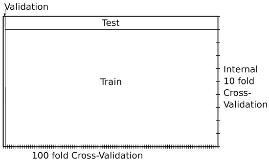
Figure 4.
Illustration of one iteration of the nested cross-validation.
After reproducing the experimentation with the 13 features selected in the original study, the GA was applied with the goal of finding a better feature set fitting more effective classifiers. In order to configure the parameters of the GA, based on previous experimentation, we adopted the values proposed in [20], which are detailed in Table 3. Since using grid search inside the wrapper cross validation (used as fitness measure) is unfeasible, the default parameters from scikit-learn were used for the classifiers and 1 nearest neighbor for kNN.
Table 3.
Parameter values fixed in the genetic algorithm.
In order to find a good setup for feature selection GA, the parameter values shown in Table 4 were tested.
Table 4.
Parameter values tested for the genetic algorithm.
As part of our comparative analysis, we also executed DE. Its parameter settings are summarized in Table 5. The control parameters F and CR were selected from commonly used default values in the DE literature, based on preliminary experiments on other datasets. The initialization strategy was aligned with that of the genetic algorithm (GA), after observing that the typical default initialization value of 0.5 yielded inferior results during preliminary testing. To ensure a comparable computational effort, the same population size and number of generations were used for both algorithms.
Table 5.
Parameter values for Differential Evolution.
5. Results Analysis
As an initial step, we replicated the experimental evaluation presented in [4], using the same 13 selected features and sticking to the same classification processes and software for all classifiers, including the kNN classifier. This replication ensures methodological consistency and enables a direct comparative analysis with the original results. The only difference is that we transformed the 100 repetitions into a second-level 100-fold cross-validation by prescinding one or two instances per repetition. Given the small number of omitted instances, their impact on the results is expected to be negligible, while it establishes a confident approach to evaluate potential improvements and assess the robustness of the models.
The results achieved using Recursive Feature Elimination (RFE) for each classifier in the original experimentation are shown in the first column of Table 6. Then, they performed a second RFE and selected 13 features as the most relevant. This is shown in the second column and it is the part of the experimentation reproduced. The classification results obtained with this subset of features in the reproduced experimentation are shown in the following columns. It is unclear to us what the value reported in the original proposal is. We believe it must be the average test accuracy of the best model found, not the average of the 100 runs over the average test, because that value is closer to the best model column in Table 6 (which is the best model according to the average of 100 repetitions of 10-fold CV test accuracies). With that consideration, the results obtained seem similar, confirming the validity of their experimentation.
Table 6.
Results from [4] compared with the models found in the experimental reproduction with 100 repetitions of the 10-fold CV using the same 13 features.
Nevertheless, it is important to note that validation indicates that the model’s expected accuracy is around 74%, which is lower than the reported best test average of 79.63% from the original study (and the 77.65% from the reproduced equivalent result). It seems that, by repeating the train–test process many times, the feature selection and the parameters of the classifiers may be overfit to the test data.
The DTC classifier achieved the highest validation accuracy (74.09%), demonstrating its effectiveness when trained with the selected features. However, the performance drop observed for the remaining classifiers between testing and validation suggests that the selected characteristics may primarily favor the DTC, potentially limiting its generalization across different models. Furthermore, it is important to note that the performance of the other classifiers does not exceed the baseline of the majority class, indicating that these models provide very poor discriminative power. To highlight this, those models with validation accuracy over the majority rate are colored in green. These results highlight the need for further analysis of the feature selection and learning process to ensure robustness and generalization.
In the second phase of our study, the GA is used to perform feature selection and evaluate its impact on the different classifiers. As an example, the evolution process of one run of the GA is illustrated in Figure 5.
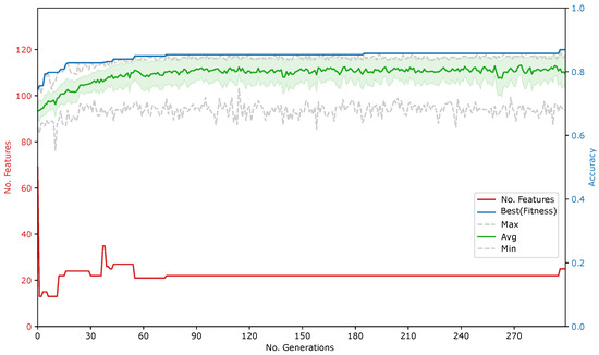
Figure 5.
Evolution of the GA wrapping DTC with a 0.3 feature set penalty and no variance penalty (fourth line of Table 7).
The results in Table 7 show that the 16 features selected by the GA wrapping RFC achieved the highest validation accuracy (71.64%) by using a penalty factor of 0.3, demonstrating that the evolutionary approach can improve the generalization capacity of the models studied, as this result is much higher than those achieved for RFC by using RFE in the previous study. In contrast, the DTC classifier, which had previously obtained the highest test accuracy, experienced a significant drop in validation, evidencing a possible overfitting of the training set, probably because it is using too many features.
Table 7.
Results using features selected by the genetic algorithm.
In the third phase, we test the hypothesis that when using Equation (2), the found feature sets are less prone to overfitting. Table 8 shows the results of the same experiments presented in Table 7 but using the new fitness calculation with a penalization for non homogeneous accuracy among test partitions. The results seem to improve but the differences are small and they cannot be considered conclusive. For this reason, we think that more research is needed to find strategies to avoid overfitting in these challenging high-dimensional datasets with few instances.
Table 8.
Results using features selected by the genetic algorithm with a fitness penalization based on the variance in CV.
Table 9 compares the different methods analyzed, including RFE, the GA approach, the variance penalty version of the GA, and DE applied to the five classifiers kNN, DTC, RFC, ETC, and XGBC. The results show that with RFE, DTC achieved the best validation accuracy (74.09%), separating itself from the other classifiers. However, in the GA and GA with variance penalty methods, RFC and XGBC showed superior performance, especially with penalties of 0.3 and 0.5. In particular, RFC achieved a remarkable validation performance (71.64%) with 16 features selected using the GA approach, while XGBC reached its maximum performance (70.35%) with 9 features and a penalty of 0.5. However, kNN showed inferior performance in most cases, although a higher penalty (0.7) improved its accuracy by selecting only four features. These results suggest that GA and GA with variance penalty methods are effective in improving generalization, especially in ensemble classifiers such as RFC and XGBC, while DTC remains the best classifier with the 13 features selected in the original study. With a similar running time, DE have not improved any of the results from RFE or GA.
Table 9.
Comparison of feature selection for each classifier based on validation results.
Although accuracy was used as the primary metric for comparison, the F1-score was also calculated to provide another assessment of model performance, given that this dataset has moderate class imbalance, which is common in medical datasets. This additional metric allows for an assessment of the balance between precision and recall in the classifiers evaluated [21]. Therefore, its inclusion complements the accuracy metric by highlighting the trade-off between false positives and false negatives, which is especially relevant in medical decision-making contexts.
F1-score () is defined as the harmonic mean of precision and recall, providing a single measure that balances both concerns, as shown in Equation (5),
where Precision is the ratio of true positive predictions to the total number of positive predictions made, as shown in Equation (6),
and Recall is the ratio of true positive predictions to the total number of actual positive instances, as shown in Equation (7).
ranges from 0 to 1, where 1 indicates perfect precision and recall and 0 indicates the worst performance. As we considered Toxic as the positive class, in this metric, the baseline established by majority classifiers, that we set to be beaten, is given by Equation (8) or (9), where p is the probability of the majoritarian class (0.6725).
As in this case the majoritarian class is the negative class (Non-toxic), any classifier with over 0 is performing better than a majority classifier with respect to detecting toxicity.
The results in Table 10 show that the best performing classifiers coincide with those identified by the accuracy metric. The values show that there is much space to improve in this challenging dataset.
Table 10.
Comparison of feature selection methods for each classifier based on validation results using the F1-score metric.
6. Conclusions
The problem addressed is highly challenging, not only because it belongs to the class of high-dimensional datasets with few instances but also because, after extensive experimentation, achieving a genuine improvement in generalization over the majority class rate with high confidence appears to be highly unlikely.
After reproducing the experiments from the paper that introduced the problem, using an independent validation, we found that the actual expected accuracy is 4% lower than the reported test accuracy. This highlights the importance of avoiding repeated testing on the same data, as it increases the likelihood of obtaining a model that performs well under a specific test setup but fails to generalize.
Using the proposed GA to automate the FS process appears promising as, although it has not been able to improve the best model found using DTC in the original study, it has improved the FS performed with RFE for most of the classification models.
The use of the proposed variance penalty in the GA’s fitness function seems promising because it has achieved several better generalization results than the non-penalized version. However, it deserves more research to finetune it and prove its performance in different datasets.
Author Contributions
Conceptualization, M.L.-R., J.M.-B. and A.A.-A.; methodology, J.M.-B.; software, J.M.-B. and A.A.-A.; validation, A.A.-A., M.L.-R. and J.M.-B.; formal analysis, M.L.-R.; investigation, J.M.-B. and A.A.-A.; resources, J.M.-B.; data curation, J.M.-B. and A.A.-A.; writing—original draft preparation, J.M.-B. and A.A.-A.; writing—review and editing, M.L.-R. and A.A.-A.; supervision, M.L.-R. and A.A.-A.; project administration, M.L.-R.; funding acquisition, A.A.-A. All authors have read and agreed to the published version of the manuscript.
Funding
This research is supported by projects PID2020-118224RB-I00, PID2023-151336OB-I00 and PID2023-148396NB-I00 funded by MICIU/AEI/10.13039/501100011033, Ministerio de Ciencia e Innovación (Spain, EU).
Data Availability Statement
The dataset used is available at: https://archive.ics.uci.edu/dataset/728/toxicity-2. Source code is available at: https://github.com/arauzo/EvolOptimizationClassification-Small-Molecules-Regulating-the-Circadian-Rhythm-Period. Experimental logs are available upon request to authors.
Conflicts of Interest
The authors declare no conflicts of interest.
Abbreviations
The following abbreviations are used in this manuscript:
| CV | Cross Validation |
| CRY1 | Cryptochrome 1 |
| DEAP | Distributed Evolutionary Algorithms in Python |
| DE | Differential Evolution |
| DTC | Decision Tree Classifier |
| ETC | Extra Trees Classifier |
| FS | Feature Selection |
| GA | Genetic Algorithm |
| kNN | k-Nearest Neighbors |
| RFC | Random Forest Classifier |
| RFE | Recursive Feature Elimination |
| XGBC | Extreme Gradient Boosting Classifier |
References
- Jagielo, A.; Benedict, C.; Spiegel, D. Circadian, hormonal, and sleep rhythms: Effects on cancer progression implications for treatment. Front. Oncol. 2023, 13, 1269378. [Google Scholar] [CrossRef] [PubMed]
- Kolarski, D.; Miller, S.; Oshima, T.; Nagai, Y.; Aoki, Y.; Kobauri, P.; Srivastava, A.; Sugiyama, A.; Amaike, K.; Sato, A. Others Photopharmacological manipulation of mammalian CRY1 for regulation of the circadian clock. J. Am. Chem. Soc. 2021, 143, 2078–2087. [Google Scholar] [CrossRef] [PubMed]
- Wildey, M.; Haunso, A.; Tudor, M.; Webb, M.; Connick, J. High-throughput screening. Annu. Rep. Med. Chem. 2017, 50, 149–195. [Google Scholar]
- Gul, S.; Rahim, F.; Isin, S.; Yilmaz, F.; Ozturk, N.; Turkay, M.; Kavakli, I. Structure-based design and classifications of small molecules regulating the circadian rhythm period. Sci. Rep. 2021, 11, 18510. [Google Scholar] [CrossRef] [PubMed]
- Chawathe, S. Attribute Selection and Visualization for Classification for Small Molecules. In Proceedings of the 2022 IEEE 13th Annual Ubiquitous Computing, Electronics and Mobile Communication Conference (UEMCON), New York, NY, USA, 26–29 October 2022; pp. 0456–0462. [Google Scholar]
- Kuncheva, L.; Matthews, C.; Arnaiz-González, Á.; Rodrıéguez, J. Feature selection from high-dimensional data with very low sample size: A cautionary tale. arXiv 2020, arXiv:2008.12025. [Google Scholar]
- Feng, G. Feature selection algorithm based on optimized genetic algorithm and the application in high-dimensional data processing. PLoS ONE 2024, 19, e0303088. [Google Scholar] [CrossRef] [PubMed]
- Luque-Rodriguez, M.; Molina-Baena, J.; Jimenez-Vilchez, A.; Arauzo-Azofra, A. Initialization of feature selection search for classification. J. Artif. Intell. Res. 2022, 75, 953–983. [Google Scholar] [CrossRef]
- Slowik, A.; Kwasnicka, H. Evolutionary algorithms and their applications to engineering problems. Neural Comput. Appl. 2020, 32, 12363–12379. [Google Scholar] [CrossRef]
- Li, T.; Dong, H.; Yin, G.; Sha, Y. An effective differential evolution with binary strategy for feature selection problem. In Proceedings of the 2019 IEEE International Conference on Systems, Man and Cybernetics (SMC), Bari, Italy, 6–9 October 2019; pp. 158–163. [Google Scholar]
- Kelly, M.; Longjohn, R.; Nottingham, K. The UCI Machine Learning Repository. 2023. Toxicity Dataset. Available online: https://archive.ics.uci.edu/dataset/728/ (accessed on 9 May 2025).
- Steinbach, M.; Tan, P. kNN: k-nearest neighbors. In The Top Ten Algorithms in Data Mining; Chapman and Hall/CRC: Boca Raton, FL, USA, 2009; pp. 165–176. [Google Scholar]
- Cover, T.; Hart, P. Nearest neighbor pattern classification. IEEE Trans. Inf. Theory 1967, 13, 21–27. [Google Scholar] [CrossRef]
- Priyanka; Kumar, D. Decision tree classifier: A detailed survey. Int. J. Inf. Decis. Sci. 2020, 12, 246–269. [Google Scholar] [CrossRef]
- Blanchet, L.; Vitale, R.; Vorstenbosch, R.; Stavropoulos, G.; Pender, J.; Jonkers, D.; Schooten, F.; Smolinska, A. Constructing bi-plots for random forest: Tutorial. Anal. Chim. Acta 2020, 1131, 146–155. [Google Scholar] [CrossRef] [PubMed]
- Sharaff, A.; Gupta, H. Extra-tree classifier with metaheuristics approach for email classification. In Advances in Computer Communication and Computational Sciences: Proceedings of IC4S 2018; Springer: Singapore, 2019; pp. 189–197. [Google Scholar]
- Chen, T.; He, T.; Benesty, M.; Khotilovich, V.; Tang, Y.; Cho, H.; Chen, K.; Mitchell, R.; Cano, I.; Zhou, T. Xgboost: Extreme gradient boosting. R Package Version 0.4–2 2015, 1, 1–4. [Google Scholar]
- Fortin, F.; De Rainville, F.; Gardner, M.; Parizeau, M.; Gagné, C. DEAP: Evolutionary algorithms made easy. J. Mach. Learn. Res. 2012, 13, 2171–2175. [Google Scholar]
- Pedregosa, F.; Varoquaux, G.; Gramfort, A.; Michel, V.; Thirion, B.; Grisel, O.; Blondel, M.; Prettenhofer, P.; Weiss, R.; Dubourg, V. Others Scikit-learn: Machine learning in Python. J. Mach. Learn. Res. 2011, 12, 2825–2830. [Google Scholar]
- Arauzo-Azofra, A.; Molina-Baena, J.; Jimenez-Vilchez, A.; Luque-Rodriguez, M. Simple cooperative coevolutionary genetic algorithm for feature selection in classification. 2025; Unpublished manuscript, submitted to journal Advances in Data Analysis and Classification (ADAC). [Google Scholar]
- Matharaarachchi, S.; Domaratzki, M.; Muthukumarana, S. Assessing feature selection method performance with class imbalance data. Mach. Learn. Appl. 2021, 6, 100170. [Google Scholar] [CrossRef]
Disclaimer/Publisher’s Note: The statements, opinions and data contained in all publications are solely those of the individual author(s) and contributor(s) and not of MDPI and/or the editor(s). MDPI and/or the editor(s) disclaim responsibility for any injury to people or property resulting from any ideas, methods, instructions or products referred to in the content. |
© 2025 by the authors. Licensee MDPI, Basel, Switzerland. This article is an open access article distributed under the terms and conditions of the Creative Commons Attribution (CC BY) license (https://creativecommons.org/licenses/by/4.0/).