A Novel Connected-Components Algorithm for 2D Binarized Images

Abstract

This paper introduces a new memory-efficient algorithm for connected-components labeling in binary images, which is based on run-length encoding. Unlike conventional pixel-based methods that scan and label individual pixels using global buffers or disjoint-set structures, our approach encodes rows as linked segments and merges them using a union-by-size strategy. We accelerate run detection by using a precomputed 16-bit cache of binary patterns, allowing for fast decoding without relying on bitwise CPU instructions. When compared against other run-length encoded algorithms, such as the Scan-Based Labeling Algorithm or Run-Based Two-Scan, our method achieves up to 35% faster on most real-world datasets. While other binary-optimized algorithms, such as Bit-Run Two-Scan and Bit-Merge Run Scan, are up to 45% faster than our algorithm, they require much higher memory usage. Compared to them, our method tends to reduce memory consumption on some large document datasets by up to 80%.

1. Introduction

Connected-component labeling (CCL) is a fundamental operation in image processing, computer vision, and pattern recognition, serving as a building brick for object detection, shape analysis, and segmentation tasks [1]. The notion of CCL is fundamental to various image analysis tasks, including document processing, biomedical imaging, and industrial defect detection [2,3,4].

The problem, simply put, involves identifying and labeling distinct groups of connected pixels in a binarized image. Given an input image consisting of only two pixel values, black (foreground) and white (background), the goal is to assign unique labels to clusters of connected foreground pixels while ensuring that all pixels within the same component share the same label.

Mathematically, the connected-component problem can be described as follows:

Given a binary image I defined on a 2D lattice $\Omega \subseteq { \mathrm{Z}}^2$, let $P$ be the set of all black pixels, $\mathrm{I}(\mathrm{x}, \mathrm{y})=1$. The task is to partition $P$ into maximally connected subsets ${\mathrm{C}}_{\mathrm{i}}, \mathrm{i}=\stackrel{-}{ 1,\mathrm{n}}$ such that each subset ${\mathrm{C}}_{\mathrm{i}}$ satisfies the connectivity condition: $\forall (\mathrm{p}, \mathrm{q})\in { \mathrm{C}}_{\mathrm{i}}$, there exists a sequence of pixels $\left\{{\mathrm{p}}_0, {\mathrm{p}}_1, \dots , {\mathrm{p}}_{\mathrm{k}}\right\}$ where ${\mathrm{p}}_0=\mathrm{p}, {\mathrm{p}}_{\mathrm{k}}=\mathrm{q}$, and each consecutive pair $\left({\mathrm{p}}_{\mathrm{j}}, {\mathrm{p}}_{\mathrm{j}+1}\right)$ is connected under a given neighborhood definition.

The two most common definitions of pixel connectivity in digital images are as follows:

• 4-way connectivity: A pixel is connected to its immediate vertical and horizontal neighbors.
• 8-way connectivity: A pixel is also connected to its diagonal neighbors.

Classical algorithms such as two-pass labeling [5], disjoint sets [6], and contour tracing [7] despite their simplicity and effectiveness often struggle with scalability in real-time, high-resolution applications, or on more specialized architectures due to factors such as memory overhead, inefficient cache usage, and the need for repeated image passes. Modern approaches, such as those based on dynamic data structures [8,9,10], parallelization [5,8,11], or optimized access patterns [12], have been introduced in order to address some of these issues and achieve better overall results.

1.1. Classical Labeling Approaches

The earliest algorithms for CCL relied on raster-scanning strategies, where the image is processed row by row to assign labels to connected pixels. The two-pass labeling algorithm, introduced by Rosenfeld [13], remains one of the most well-known classical approaches. It operates as follows:

• First Pass (Initial Labeling and Equivalence Table Creation): The binary image is scanned in raster order (left to right, top to bottom). Each black pixel is assigned a provisional label based on its neighboring pixels. If a pixel has multiple labeled neighbors, an equivalence table is updated to record that the labels belong to the same connected component.
• Second Pass (Label Resolution): Once the entire image has been processed, the equivalence table is resolved using a union-find data structure [14]. Each pixel is updated with the final label corresponding to its connected component.

The two-pass algorithm is widely used due to its simplicity but suffers from high memory overhead and poor cache efficiency, particularly when dealing with large images.

Another approach to CCL involves contour tracing, where connected components are identified by following their external boundaries. The algorithm introduced by Suzuki and Abe [15] follows a border-following technique, tracing connected pixel boundaries and assigning labels accordingly. This method is particularly useful for shape analysis but is computationally expensive for dense, highly connected images.

The union-find approach [14] builds on the classical two-pass algorithm but optimizes label resolution using path compression and union by rank. This results in near-constant-time complexity for label merging, significantly reducing the overhead associated with equivalence table resolution. In this method:

• Each connected component is treated as a disjoint set, and pixel labels are managed using find and union operations.
• The find operation determines the root label of a component, while the union efficiently merges components.

Although union-find is more memory efficient than classical two-pass algorithms, it still requires multiple scans of the image and is difficult to parallelize effectively.

1.2. Run-Length-Based Methods

Run-Length Encoding (RLE) methods address the inefficiencies of pixel-wise algorithms by grouping consecutive black pixels into runs and processing them at a higher abstraction level. These approaches were first explored by Haralock and Shapiro [16] and have been further developed in recent years.

RLE is a technique where contiguous sequences of identical values are stored as runs instead of individual pixel values. For a binary image, this means that black pixels in each row are stored as (start, end) coordinate pairs. For example, in a row with pixels $[0 0 1 1 1 0 0 1 1 0 0 0]$, the run-length representation is $\left[\right(\mathrm{2,4}), (\mathrm{7,8}\left)\right]$.

Instead of assigning labels to individual pixels, run-length-based algorithms operate on runs, significantly reducing the number of comparisons needed. The process follows these steps:

• Extract all black runs per row: Each sequence of consecutive black pixels is stored as a run.
• Create run-length structures: Each run is initially treated as an independent component.
• Merge connected runs across rows: Runs are linked based on 4-way or 8-way connectivity rules.

Let $\mathrm{R}(\mathrm{x}, \mathrm{y}, \mathrm{w})$ be a run starting at pixel $(\mathrm{x}, \mathrm{y})$ with width w. Runs R₁ and R₂ from successive rows are merged if ${\mathrm{x}}_1 \le {\mathrm{x}}_2+{\mathrm{w}}_2$ and ${\mathrm{x}}_1+{\mathrm{w}}_1 \ge {\mathrm{x}}_2$ (for 4-way connectivity), or additionally $|{\mathrm{x}}_1-{ \mathrm{x}}_2| \le 1$ (for 8-way connectivity).

This method significantly reduces the number of label updates compared to pixel-wise methods and is well-suited for parallelization on modern architectures [17].

1.3. Modern Connected-Component Labeling Methods

More recent advances in CCL have focused on parallel processing, GPU acceleration, and machine learning-driven optimizations. Some key methods include the following:

Modern CCL implementations leverage parallelization and powerful architectures to perform labeling [5,8,11]. These methods divide the image into tiles, process labels independently, and merge results in a post-processing step. While effective for real-time applications, they require specialized hardware and are challenging to implement on CPU-based systems.

Graph-based CCL treats the image as a connectivity graph, where pixels are nodes, and edges represent connectivity relationships [10]. These methods use graph-cut techniques for efficient segmentation but are computationally expensive for large datasets.

An interesting extension of CCL allows for images where the foreground does not have a constant color. He et al. [18] performed complex object segmentation using a convolutional neural network (CNN) to predict component labels directly from image pixels. Methods such as this excel in handling complex textures but require large, labeled datasets for training. Region-merging approaches iteratively combine neighboring labeled regions using statistical or geometric criteria [19]. These methods are particularly useful for noisy or degraded images, where classical pixel-based approaches fail.

In this paper, we introduce an RLE-based method that uses a combination of segment precaching, image traversal by groups of pixels, instead of individually looking at each one at a time, combined with a specialized segment traversal and merge approach, in order to obtain the final structure that can be used for labeling. The advantages of some of these steps include reduced memory overhead, efficient component merging, and scalability.

In Section 2, we present the data structures and the steps used in the proposed algorithm, and we discuss two algorithm variants. In Section 3, we describe the evaluation methodology and compare the results of the proposed algorithm with other state-of-the-art algorithms. In Section 4, we present a discussion based on these results and draw conclusions.

2. Materials and Methods

The proposed method presents an efficient approach for CCL in binarized 2D images. By leveraging RLE and self-pointer structures, the algorithm significantly reduces the number of comparisons required for labeling, leading to improved computational efficiency and lower memory consumption. This section provides a detailed explanation of the method, including the run-length generation process, component linking structures, merging strategy, and the handling of 4-way and 8-way connectivity.

2.1. Run-Length Generation Process

As previously introduced, RLE is a technique used to represent sequences of consecutive identical values. In the context of binary images, RLE identifies continuous horizontal sequences of black pixels (foreground pixels, value 1) and encodes them as run segments. Each run is characterized by a starting coordinate, an ending coordinate, and the row index: $\mathrm{R}({\mathrm{x}}_{\mathrm{s}}, {\mathrm{x}}_{\mathrm{e}}, \mathrm{y})$ represents a continuous sequence of black pixels starting at position ${\mathrm{x}}_{\mathrm{s}}$, ending at ${\mathrm{x}}_{\mathrm{e}}$, and located in row $\mathrm{y}$. In the following algorithms, ${\mathrm{x}}_{\mathrm{s}}$ is dentoted as $run.start$, $x_e$ as $run.end$, and $y$ as $run.row$. Mathematically, a run ${\mathrm{R}}_{\mathrm{i}}$ is defined as ${\mathrm{R}}_{\mathrm{i}}=({\mathrm{x}}_{\mathrm{si}}, {\mathrm{x}}_{\mathrm{ei}}, {\mathrm{y}}_{\mathrm{i}})$, where $\mathrm{I}(\mathrm{x}, \mathrm{y})=1$ for $\mathrm{x} \in [{\mathrm{x}}_{\mathrm{si}}, {\mathrm{x}}_{\mathrm{ei}}]$ and $\mathrm{I}({\mathrm{x}}_{\mathrm{s}} - 1, \mathrm{y})=\mathrm{I}({\mathrm{x}}_{\mathrm{e}}+1, \mathrm{y})=0$.

In our case, unlike traditional RLE-based CCL algorithms, which process image pixels one at a time, our algorithm pre-caches a precomputed lookup table used to extract runs from words that represent binary pixels. Each row gets interpreted in sequences of 16-bit integers, where each bit encodes a pixel. This step allows for rapid segmentation of rows by simply looking up segment patterns and offsetting them accordingly.

In order to achieve this, we construct a CacheSegment table, obtained after executing a one-time preprocessing phase. All 65,536 possible 16-bit values get scanned and, for each one, the positions of 0-bit runs are identified and stored as initial one-pixel segments. This result is then further refined by a second pass, which merges adjacent or overlapping segments into possible RLEs. It is important to mention that since this table caches all possible 16-bit runs that could be identified in an image, it only needs to be computed once on program startup.

This merging is implemented as a linear scan through the generated segments, performed in reverse. If any pair of consecutive segments is found where the end of the first would touch the start of the second, they are merged in place by adjusting segment boundaries. The segment list is then memory-shifted in place in order to remove the redundant entry. These steps ensure a compact lookup table that stores only valid horizontal runs for each 16-bit word. The steps for this method can be seen in Algorithm 1.

Algorithm 1. Precompute Segment Caching Algorithm
Input: None
Output: CacheSegments—map of 16 bits to horizontal runs
1.	For wordValue ← 0:65,535
2.	Segments ← empty list
3.	For i ← 0 to 15 do
4.	If wordValue[i] = 1
5.	start ← i
6.	end ← i
7.	Segments.append((start, end))
8.	i ← size(Segments) − 2
9.	While i ≥ 0
10.	If Segments[i].end + 1 ≥ Segments[i + 1].start
11.	Segments[i].end ← Segments[i + 1].end
12.	Remove Segments[i + 1] by shifting the remaining entries left
13.	Decrease size(Segments)
14.	Else
15.	i ← i − 1
16.	CacheSegments[wordValue] ← Segments

Following the CacheSegments creation, we proceed to extract RLE from the image rows by looking at the pixels in a row in 16-bit increments. This can be seen in Algorithm 2.

Algorithm 2. Run-Length Generation Pseudocode
Input: Binary Image
Output: List or row-wise RLE segments
1.	For row ← 0:height-1
2.	imageRow ← image[row]
3.	RowSegments ← empty list
4.	imageWidthWords ← width/16
5.	For i ← 0:imageWidthWords-1
6.	word ← imageRow[i]
7.	Segments ← CacheSegments[i]
8.	For each segment in Segments
9.	start← 16×i + segment.start
10.	end← 16×i + segment.end
11.	RowSegments.append((start, end, row))

2.2. Data Structures for Component Linking

Instead of treating individual pixels as elements in a connected component, the proposed method operates on runs, which significantly reduces the number of operations required for component merging. To efficiently store and link runs into connected components, we introduce a self-pointer structure, where the elements of each run-node are described in

Table 1. Run-node elements.

Element	Description	Notation	Initial Value
Run	A reference to its own run	$N_i.run$	$R_i$
Head	A pointer to the first run in the component	$N_i.head$	$N_i$
Next	A pointer to the next run within the same component	$N_i.next$	NULL
Size	A counter indicating the number of runs in the component	$N_i.size$	1
Label	A number indicating the label of the component	$N_i.label$	NULL

.

These nodes are stored in a run vector, ordered row-wise, forming an implicit raster structure.

2.3. Merging Connected Components Across Rows

Once all runs have been extracted and stored in the run vector, adjacent rows are scanned pairwise to merge connected runs based on 4-way or 8-way connectivity rules.

To determine whether two runs ${\mathrm{R}}_{\mathrm{i}}\left({\mathrm{x}}_{\mathrm{si}}, {\mathrm{x}}_{\mathrm{ei}}, {\mathrm{y}}_{\mathrm{i}}\right)$ and ${\mathrm{R}}_{\mathrm{j}}\left({\mathrm{x}}_{\mathrm{sj}}, {\mathrm{x}}_{\mathrm{ej}}, {\mathrm{y}}_{\mathrm{j}}\right)$ belong to the same connected component, the following conditions are checked:

• For 4-way connectivity: ${\mathrm{R}}_{\mathrm{i}}$ and ${\mathrm{R}}_{\mathrm{j}}$ are connected if they overlap horizontally and are located in consecutive rows, meaning ${\mathrm{x}}_{\mathrm{sj}} \le { \mathrm{x}}_{\mathrm{ei}}$ and ${\mathrm{x}}_{\mathrm{si}} \le {\mathrm{x}}_{\mathrm{ej}}$ for ${\mathrm{y}}_{\mathrm{j}}={ \mathrm{y}}_{\mathrm{i}}+1$.
• For 8-way connectivity: ${\mathrm{R}}_{\mathrm{i}}$ and ${\mathrm{R}}_{\mathrm{j}}$ are connected if they satisfy 4-way connectivity or are diagonally adjacent, meaning $|{\mathrm{x}}_{\mathrm{sj}}-{\mathrm{x}}_{\mathrm{ei}}| \le 1$ or $|{\mathrm{x}}_{\mathrm{si}}-{\mathrm{x}}_{\mathrm{ej}}| \le 1$ for ${\mathrm{y}}_{\mathrm{j}} = {\mathrm{y}}_{\mathrm{i}}+1$.

If two runs ${\mathrm{R}}_{\mathrm{i}}$ and ${\mathrm{R}}_{\mathrm{j}}$ satisfy the connectivity condition, their corresponding nodes N_i and N_j are merged using the strategy presented in Algorithm 3. This merging strategy ensures efficient union operations, leveraging the union by size heuristic to maintain a balanced component structure. Something to note is that we create two separate lists that are intended to keep track of the start and end segments for each row, allowing us to iterate faster over rows, by either skipping empty rows or determining quickly if there are no more segments on the current one.

Algorithm 3. Merge Strategy Pseudocode
Input: List of RLE segments
Output: List of connected components
1.	rowStart, rowEnd ← List(totalRows,null)
2.	connectivity ← 1 if 8-connected else 0
3.	For each segment in RowSegments:
4.	If rowStart[segment.row] = null
5.	rowStart[segment.row] = segment
6.	rowEnd[segment.row] = segment
7.	For row = 1:totalRows
8.	If current row or previous row has no segments
9.	skip
10.	curr←rowStart[row]
11.	currEnd←rowEnd[row]
12.	upper←rowStart[row-1]
13.	upperEnd←rowEnd[row-1]
14.	While curr! = currEnd AND upper! = upperEnd
15.	If curr.run.end + connectivity < upper.run.start
16.	curr←curr+1
17.	Else If curr.run.start – connectivity > upper.run.end
18.	upper←upper+1
19.	Else
20.	If curr.head! = upper.head
21.	If curr.head.size > upper.head.size
22.	Swap(curr,upper)
23.	upper.head.size ← upper.head.size + curr.head.size
24.	For(walk←curr.head;walk.next! = null;walk ← walk.next)
25.	walk.head ← upper.head
26.	walk.head ← upper.head
27.	walk.next ← upper.head.next
28.	upper.head.next←current.head
29.	If curr.run.end + connectivity < upper.run.end
30.	curr←curr + 1
31.	Else
32.	upper←upper + 1

2.4. Extraction of Connected Components

Once all rows have been processed, connected components are extracted via Algorithm 4. The final output is a labeled image where each connected component is uniquely identified.

Algorithm 4. Connected Component Labeling Pseudocode
Input: List of connected components
Output: Labeled image
1.	For i = 1:RunList.Length
2.	$N_i\leftarrow$RunList(i).First
3.	$\mathbf{If} N_i.head=N_i$
4.	Do
5.	$N_i.label\leftarrow i$
6.	$N_i\leftarrow N_i.next$
7.	$\mathbf{While} N_i$! = NULL

2.5. Discussion on 4-Way vs. 8-Way Connectivity

The choice between 4-way and 8-way connectivity significantly impacts the number of connected components and algorithm complexity.

While 4-way connectivity tends to produce more distinct components, 8-way connectivity captures diagonal connections and reduces fragmentation, making it more suitable for natural images and complex structures.

The proposed method describes the approach of the authors’ patented application for identifying connected components in binary images [20]. Since the original patent documentation is available only in Romanian, the present article offers a comprehensible, self-contained description of the said algorithm in order to improve its overall accessibility. However, it is important to note that additional optimizations and tests were performed compared to the original code, adding a variety of improvements in certain scenarios.

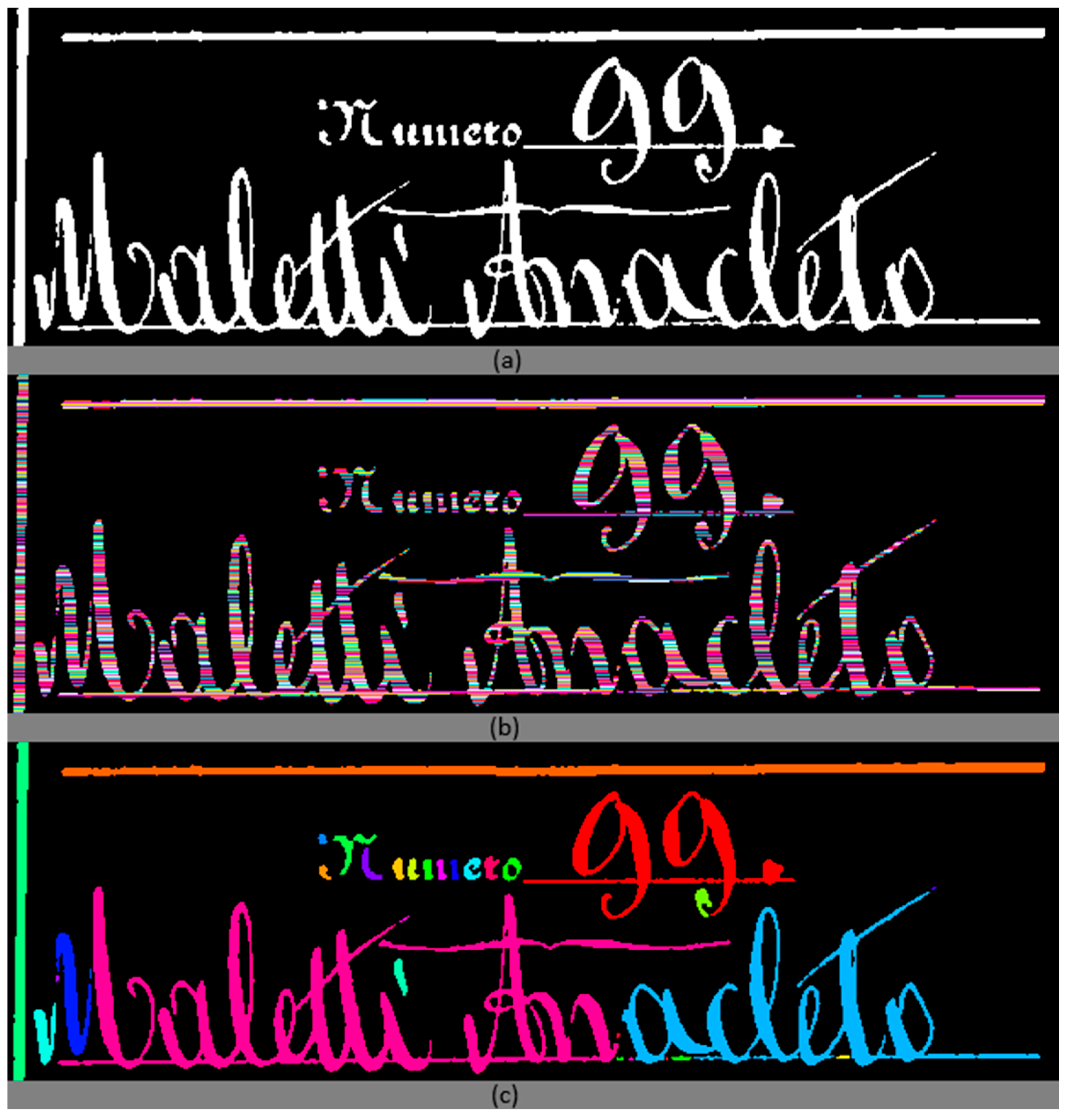
Figure 1 shows an example image, going through the run-lengths generation and then through merging using 8-way connectivity. The run segments and connected components were assigned random colors to easily visualize them. The three images are separated by horizontal gray bars.

3. Results

This section presents the experimental evaluation of the proposed method, detailing the experimental setup, dataset characteristics, performance metrics, comparative analysThe colors do not need additional explanation. They just aid in distinguishing the connected components and RLE segments is against state-of-the-art algorithms, and potential limitations with avenues for improvement. The focus is on execution speed and memory efficiency, as these factors play a critical role in the applicability of CCL in real-world scenarios.

3.1. Experimental Setup and Datasets

To assess the performance of the proposed run-length-based approach, we implemented the method in C++ and compared it against well-established CCL techniques using the YACCLAB [21,22,23] benchmark. Specifically, we evaluated our approach against Scan Array Union-Find (SAUF) Algorithm [8], Block-Based Decision Tree (BBDT) [24], Pixel Prediction (PRED) [25], Directed Rooted Acyclic Graphs (DRAG) based scanning [26], and Spaghetti [9]. Additionally, we also test a variety of algorithms that work specifically on RLE, such as Stripe-Based Labeling Algorithm (SBLA) [27], Run-Based Two-Scan (RBTS) [28], and more modern ones that use bit-level processing, such as Bit-Run Two Scan (BRTS) and Bit-Merge-Run Scan (BMRS) proposed by Lee et al. [29]. All algorithms tested, except for ours, were employed to use a Union Find with Path Compression structure (UFPC) when solving labels, as that tended to perform the best in our tests.

We test all algorithms on some of the datasets provided by YACCLAB, which contain a variety of black-and-white binary images, as well as a synthetic one with varying degrees of density between black and white. One thing to note is that this dataset is a subset of the classical big dataset found in YACCLAB, but only includes the large images for a better overall assessment. The details for these datasets are given in

Table 2. Datasets used for testing.

Dataset	Total Images	Description	Approximate Resolution
Fingerprints [30]	960	Collection of fingerprints	300 × 300
Hamlet [31]	105	Scanned images pertaining to Shakespeare’s Hamlet	1200 × 2175
Medical [32]	343	Various images of anatomical structures	Very different sizes: [800–1900] × [750–900]
3dpes [33]	23,189	Camera images that captured pedestrians	704 × 576
Tobacco800 [34,35]	1290	Scanned legal business documents	Small: 1200 × 1600 Large: 2400 × 3200
xDocs [36,37]	1677	Scanned documents	4700 × 3200
Mirflickr [38]	25,000	Artistic real-world images	500 × 333
Synthetic [22]	90	Collection of artificially generated images of different densities, varying from 0.1 to 0.9	4096 × 4096

.

The datasets were selected to ensure a wide range of connectivity patterns, including dense and sparse distributions of foreground pixels, to thoroughly evaluate the adaptability of each method.

All experiments were conducted on a PC with an AMD Ryzen 9 7900X3D processor, 64 GB RAM, running Windows 11 Pro 24H2 with OpenCV 4.11. The methods were compiled with Microsoft Visual Studio 2022 update 17.13.6 using optimization flags (-O2) for performance consistency, as well as extended AVX instructions. All tests were performed on 8-connectivity only, due to the fact that the variety in performance obtained when compared to 4-connectivity is minimal.

3.2. Performance Metrics

The evaluation focused on the following primary metrics:

• Mean execution time: measured in milliseconds, including the standard deviation across the dataset, in order to indicate consistency.
• Memory Usage: measured in megabytes (MB), this metric reflects the peak memory allocated by each algorithm.
• Memory accesses: the number of times each algorithm required a memory access, measured via a hardware counter.

3.3. Comparative Analysis of Algorithms

Table 3. Average total execution time per image (milliseconds) against the tested CCL algorithms.

	Dataset	Fingerprints	Hamlet	Medical	3dpes	Tobacco	xDocs	Mirflickr	Synthetic
Method
NULL		0.03 ± 0.01	1.19 ± 0.13	0.55 ± 0.11	0.3 ± 0.04	1.93 ± 1.18	6.4 ± 1.31	0.02 ± 0.01	6.54 ± 0.50
SAUF		0.22 ± 0.08	3.92 ± 0.33	1.78 ± 0.77	0.49 ± 0.06	5.61 ± 3.57	20.55 ± 2.65	0.23 ± 0.08	62.04 ± 20.94
BBDT		0.2 ± 0.08	3.82 ± 0.34	1.62 ± 0.71	0.44 ± 0.07	5.45 ± 3.32	19.42 ± 2.80	0.20 ± 0.07	49.54 ± 14.43
PRED		0.21 ± 0.08	3.7 ± 0.30	1.68 ± 0.73	0.47 ± 0.06	5.49 ± 3.35	19.76 ± 2.48	0.21 ± 0.07	57.52 ± 19.99
DRAG		0.21 ± 0.08	3.9 ± 0.43	1.65 ± 0.72	0.45 ± 0.07	5.65 ± 3.55	19.83 ± 2.61	0.19 ± 0.07	50.32 ± 14.28
Spaghetti		0.18 ± 0.07	3.11 ± 0.26	1.36 ± 0.59	0.37 ± 0.06	4.45 ± 2.86	15.98 ± 2.27	0.16 ± 0.06	45.14 ± 12.97
SBLA		0.41 ± 0.12	6.31 ± 0.56	3.13 ± 0.98	0.81 ± 0.19	10.11 ± 4.63	42.67 ± 6.32	0.48 ± 0.12	116.07 ± 29.33
RBTS		0.27 ± 0.11	4.22 ± 0.48	1.88 ± 0.74	0.52 ± 0.06	5.88 ± 3.68	22.22 ± 3.18	0.26 ± 0.08	85.94 ± 25.21
BRTS		0.11 ± 0.04	2.07 ± 0.46	0.99 ± 0.44	0.24 ± 0.06	2.71 ± 1.76	9.96 ± 1.86	0.09 ± 0.04	41.01 ± 11.57
BMRS		0.13 ± 0.05	2.05 ± 0.46	1.06 ± 0.43	0.26 ± 0.06	2.74 ± 1.78	10.25 ± 1.89	0.11 ± 0.04	43.18 ± 12.28
Proposed		0.17 ± 0.09	2.47 ± 0.28	1.03 ± 0.44	0.32 ± 0.06	3.31 ± 2.08	14.82 ± 2.09	0.15 ± 0.06	86.98 ± 27.31

shows the average execution time per image for the proposed method and compares it against the three aforementioned CCL algorithms, being measured for 10 runs, taking the minimum average across those runs, for each dataset. We use NULL to represent the ideal algorithm, one that just copies the pixels from the input image into the output image.

One thing to note is that the label image memory assignment will introduce unnecessary memory allocation overhead, this being true for all algorithms being compared. Thus, for fairness,

Table 4. Average execution time per image (milliseconds) against the tested CCL algorithms without memory allocation overhead.

	Dataset	Fingerprints	Hamlet	Medical	3dpes	Tobacco	xDocs	Mirflickr	Synthetic
Method
NULL		0.01 ± 0.003	0.29 ± 0.07	0.11 ± 0.03	0.02 ± 0.01	0.58 ± 0.32	2.52 ± 0.38	0.01 ± 0.002	2.58 ± 0.33
SAUF		0.19 ± 0.06	2.65 ± 0.28	1.21 ± 0.52	0.31 ± 0.05	3.75 ± 2.51	14.99 ± 1.88	0.21 ± 0.08	56.45 ± 20.84
BBDT		0.17 ± 0.05	2.56 ± 0.28	1.04 ± 0.45	0.25 ± 0.06	3.6 ± 2.36	13.87 ± 2.02	0.18 ± 0.06	43.95 ± 14.22
PRED		0.18 ± 0.05	2.47 ± 0.23	1.09 ± 0.47	0.28 ± 0.05	3.63 ± 2.39	14.21 ± 1.68	0.19 ± 0.07	51.93 ± 19.76
DRAG		0.18 ± 0.05	2.63 ± 0.37	1.07 ± 0.46	0.26 ± 0.06	3.79 ± 2.44	14.29 ± 1.88	0.18 ± 0.06	44.68 ± 14.04
Spaghetti		0.15 ± 0.04	1.87 ± 0.19	0.78 ± 0.34	0.18 ± 0.05	2.59 ± 1.71	10.45 ± 1.44	0.14 ± 0.06	39.59 ± 12.28
SBLA		0.39 ± 0.1	5.41 ± 0.47	2.69 ± 0.73	0.64 ± 0.17	8.76 ± 3.65	38.42 ± 4.77	0.47 ± 0.13	112.2 ± 28.26
RBTS		0.24 ± 0.08	2.97 ± 0.38	1.3 ± 0.51	0.33 ± 0.08	4.01 ± 2.75	16.65 ± 2.48	0.24 ± 0.09	80.34 ± 23.69
BRTS		0.07 ± 0.04	0.72 ± 0.13	0.37 ± 0.34	0.04 ± 0.02	0.74 ± 0.45	3.97 ± 0.77	0.07 ± 0.01	32.83 ± 10.59
BMRS		0.09 ± 0.05	0.71 ± 0.13	0.43 ± 0.34	0.05 ± 0.02	0.76 ± 0.46	4.01 ± 0.79	0.09 ± 0.02	35.97 ± 11.45
Proposed		0.15 ± 0.05	1.29 ± 0.21	0.55 ± 0.26	0.13 ± 0.07	1.55 ± 1.23	8.36 ± 1.67	0.14 ± 0.05	69.13 ± 23.38

showcases the average execution times for each algorithm with these memory allocation overheads taken out.

In addition to execution times, we measured the peak memory usage of each algorithm across a multitude of runs. We chose to avoid measuring the mean, as memory is very dependent on the operating system and device used, and we are more interested in the upper bound. Similarly, since most algorithms allocate the bulk of their memory upfront for each image, the memory does not vary that much after the first steps. The results are given in

Table 5. Peak memory allocation (in Megabytes) per dataset for each CCL algorithm.

	Dataset	Fingerprints	Hamlet	Medical	3dpes	Tobacco	xDocs	Mirflickr	Synthetic
Method
SAUF		5	55	30	13	166	385	13	319
BBDT		6	58	31	16	164	400	15	325
PRED		6	62	31	16	167	416	15	325
DRAG		6	56	29	16	168	414	15	324
Spaghetti		6	59	32	16	168	411	13	324
SBLA		8	54	38	14	156	308	12	296
BRTS		10	65	46	18	227	489	18	393
BMRS		9	67	49	18	231	495	18	395
Proposed		3	14	41	13	81	100	12	252

.

Similarly, for each algorithm, we were also interested in how many times they access the memory in total, since the fewer memory accesses required, the faster an algorithm will tend to perform, in theory. The results of these tests are given in

Table 6. Total number of memory accesses performed by each algorithm.

	Dataset	Fingerprints	Hamlet	Medical	3dpes	Tobacco	xDocs	Mirflickr	Synthetic
Method
SAUF		$8.1\times {10}^5$	$1.4\times {10}^7$	$7.1\times {10}^6$	$2.1\times {10}^6$	$2.4\times {10}^7$	$8.8\times {10}^7$	$1.2\times {10}^6$	$1.3\times {10}^8$
BBDT		$5.7\times {10}^5$	$1\times {10}^8$	$4.8\times {10}^6$	$1.5\times {10}^6$	$1.7\times {10}^7$	$6.1\times {10}^7$	$7.8\times {10}^5$	$9\times {10}^7$
PRED		$8\times {10}^5$	$1.4\times {10}^7$	$7\times {10}^6$	$1.1\times {10}^6$	$2.4\times {10}^7$	$8.8\times {10}^7$	$1.2\times {10}^6$	$1.2\times {10}^8$
DRAG		$8\times {10}^5$	$1.4\times {10}^7$	$7\times {10}^6$	$1.1\times {10}^6$	$2.4\times {10}^7$	$8.8\times {10}^7$	$1.2\times {10}^6$	$1.2\times {10}^8$
Spaghetti		$5.6\times {10}^5$	$1\times {10}^7$	$4.8\times {10}^6$	$1.5\times {10}^6$	$1.7\times {10}^7$	$6.1\times {10}^7$	$7.8\times {10}^5$	$8.7\times {10}^7$
SBLA		$7.4\times {10}^5$	$1.2\times {10}^7$	$6.5\times {10}^6$	$1.6\times {10}^6$	$2\times {10}^7$	$7.5\times {10}^7$	$1.1\times {10}^6$	$1.2\times {10}^8$
BRTS		$4.2\times {10}^5$	$8.2\times {10}^6$	$3.6\times {10}^6$	$1.2\times {10}^6$	$1.4\times {10}^7$	$5\times {10}^7$	$5.5\times {10}^5$	$5.9\times {10}^7$
BMRS		$4.6\times {10}^5$	$8.4\times {10}^6$	$3.9\times {10}^6$	$1.2\times {10}^6$	$1.4\times {10}^7$	$5.2\times {10}^7$	$6.3\times {10}^5$	$6.6\times {10}^7$
Proposed		$6.7\times {10}^5$	$5.9\times {10}^6$	$2.7\times {10}^6$	$1.4\times {10}^5$	$2.7\times {10}^6$	$1.3\times {10}^7$	$4\times {10}^5$	$5.5\times {10}^{10}$

. One thing to note is that the RBTS algorithm is missing from both of these tables because it does not have a memory test implementation in YACCLAB.

4. Discussion

This section interprets the experimental results presented earlier, analyzing some of the strengths and potential limitations of the proposed method. We identify scenarios where the method performs well and present some justifications and insights into this behavior, as well as scenarios where the method underperforms and propose directions for optimization and future research.

4.1. Comparative Performance

The proposed method consistently achieves faster execution times than most algorithms it was tested against, across a broad range of image types, with a couple of exceptions. On datasets that contain large-resolution images, such as Hamlet, Tobacco, xDocs, and Medical, our algorithm tends to heavily outperform every other one, obtaining improvements between 20% and 50% over Spaghetti. These gains are likely due to the fact that we operate at run level, rather than pixel level, in combination with the efficient merging strategy that leverages pointer-based data structures.

It is important to mention that our algorithm loses in terms of speed to other algorithms that read the image using bit-level operations, such as BRTS and BMRS. Against those algorithms, we tend to be around 50% slower.

One thing to note is that, while all other algorithms are evaluated using a UFPC as a backend for resolving label equivalences, our method uses a different merging mechanism, namely, a linked-list-based union-by-size approach. When two components are merged, the smaller list of nodes is traversed, and each node’s head pointer is updated directly. This allows skipping recursive find operations and the extra logic used in maintaining balanced trees, which are inherent in UFPC. While this merge can vary in performance, when the list of segments that need to be compared is small, such as in the case of sparse or dense images, the reduced number of memory accesses, minimal branching, and better cache behavior push it to the top.

On the other end, on datasets that contain very small images, such as Fingerprints or mirflickr, or those that contain extremely sparse ones, such as 3dpes, our algorithm still outperforms the vast majority of the rest and ties or is very close in performance to Spaghetti. This is likely due to the fact that pre-caching and other sorts of optimizations are not that beneficial, due to the small size of the images, allowing for algorithms that go directly to traversing the image to come ahead.

One major downside of our algorithm is its performance on the Synthetic dataset, which contains some images of mixed density. For these images, when the density is around 50%, the number of runs that contain a very small number of pixels will increase exponentially. In such cases, our algorithm is ill-equipped to deal with such a scenario, creating very large lists of pixels, and making UFPC approaches more efficient. However, while this is a limitation, it is not applicable to most real-world scenarios.

4.2. Memory Efficiency and Access Patterns

The proposed method demonstrates not only strong computational performance but also consistent memory efficiency. Using pre-allocated run structures stored in cache memory reduces both peak memory usage and memory fragmentation. On high-resolution datasets such as xDocs or Tobacco, the algorithm uses significantly less memory than the others, achieving savings of over 50% in some cases. It is important to mention that the other algorithms all tend to have similar peak memory usage. This is likely due to the UFPC structure needing to allocate the memory for its solution, rather than the algorithms consuming most of their memory during segment retrieval.

Something to note is that while other RLE algorithms might be faster than ours, such as BRTS and BMRS, they tend to have a very large memory footprint, especially on datasets with large images, such as xDocs, consuming close to 500 MB at peak memory usage. Meanwhile, our algorithm sits at a fifth of the memory usage, reaching only 100 MB at its peak.

However, our algorithm tends to be less suited to noisy images, as demonstrated on the Synthetic dataset, where very short and numerous runs introduce overhead that increases both execution time and the number of memory access patterns by orders of magnitude when compared to the other algorithms. This could be considered an expected trade-off, and some future developments could consider switching to a different merging or labeling structure when encountering highly fragmented images.

4.3. Comparison with RLE-Based Methods

The proposed method shares a common RLE foundation with a couple of other state-of-the-art algorithms, such as SBLA [27], RBTS [28], BRTS, and BMRS [29]. However, there are key implementation differences that distinguish our approach.

In the case of RBTS and SBLA, they use structured tables or buffers in order to manage runs and provide provisional labels across rows. RBTS, for example, uses a circular buffer of run descriptors and a compact equivalence table. Similarly, SBLA relies on scan-based merging and traversing rows across stripes.

In contrast, our method employs a pointer-linked segment structure where each run is represented as a lightweight object with references to its head component and the next segment after it for faster traversal. Merging is done via a union-by-size heuristic using direct pointer reassignment, without requiring circular buffers or label tables. This, in turn, offers simpler memory management and allows for a possible faster traversal of the overall structure, especially in sparse images.

Additionally, algorithms like BRTS and BMRS operate in a similar manner to our algorithm when computing the initial run segments by traversing the image in a bitwise fashion. More specifically, they use 64-bit operators and rely on methods such as Fast Forward Scan or masked bit OR in order to merge and detect runs in binary images. While we also process runs in a bitwise fashion, our method relies on a precomputed segment cache that allows us to decode all 16-bit binary patterns in constant time.

While both BRTS and BMRS perform faster in every scenario, they also tend to consume the most memory. In contrast, while our algorithm is slower, the lower memory footprint, due to pointer-linked structures, makes it better suited to scenarios that contain very large input images or constrained hardware environments.

5. Conclusions

The paper presents a novel RLE CCL algorithm optimized for speed, memory efficiency, and scalability. By processing horizontal runs, rather than individual pixels, and employing a direct pointer-based merging strategy, the method achieves significant improvements over traditional algorithms, such as SAUF, BBDT, and Spaghetti, particularly on sparse or moderately dense datasets and those with high-resolution images.

The proposed approach is not only much faster than some of the aforementioned algorithms by up to 50% in certain scenarios but also offers a lower memory footprint and better cache locality, offering a variety of advantages to real-world image processing tasks and making it suitable for memory-constrained environments. The relationships between runs are adjusted without modifying the memory layout, leading to fast updates without memory fragmentation. Additionally, our proposed method can be considered suitable for large-scale image processing applications, particularly in high-resolution document analysis, industrial inspection, and medical imaging.

Despite its strengths, the method does show its limitations, particularly when processing high-density, fragmented images, such as those in the Synthetic dataset. The creation of many short runs in such images leads to an increase in merging operations, impacting the overall performance.

While both 4- and 8-way connectivity are supported in the current implementation, diagonal merging is not yet as optimized as block-based methods. Thus, future work could investigate quad-tree-based merging heuristics to improve performance under 8-way connectivity, particularly in images with irregular component shapes.

Another area for enhancement lies in parallel execution. The current implementation is CPU-bound and sequential, but the algorithm is inherently parallelizable. Processing independent image tiles, followed by merging across region boundaries, could allow for efficient multithreaded execution or GPU-based acceleration.

Similarly, one improvement could be considered by precomputing a 24-bit cache table instead of a 16-bit one and traversing the image in 24-bit segments. While this would further increase the total memory footprint of the application, jumping from 65 KB to 16 MB, the increase is not that significant if we are to process larger images. Additionally, on modern CPUs, this would still be able to fit in the L1 cache without many issues, allowing for much faster processing with a limited trade-off.

References

- He, L.; Ren, X.; Gao, Q.; Zhao, X.; Yao, B.; Chao, Y. The connected-component labeling problem: A review of state-of-the-art algorithms. Pattern Recognit. 2017, 70, 25–43. [Google Scholar] [CrossRef]
- Mittal, M.; Verma, A.; Kaur, I.; Kaur, B.; Sharma, M.; Goyal, L.M.; Roy, S.; Kim, T.H. An efficient edge detection approach to provide better edge connectivity for image analysis. IEEE Access 2019, 7, 33240–33255. [Google Scholar] [CrossRef]
- Alqudah, A.M.; Alqudah, A. Improving machine learning recognition of colorectal cancer using 3D GLCM applied to different color spaces. Multimed. Tools Appl. 2022, 81, 10839–10860. [Google Scholar] [CrossRef]
- Min, Y.; Li, J.; Li, Y. Rail Surface Defect Detection Based on Improved UPerNet and Connected Component Analysis. Comput. Mater. Contin. 2023, 77, 941–962. [Google Scholar] [CrossRef]
- Gupta, S.; Palsetia, D.; Patwary, M.M.A.; Agrawal, A.; Choudhary, A. A new parallel algorithm for two-pass connected component labeling. In Proceedings of the 2014 IEEE International Parallel & Distributed Processing Symposium Workshops, Phoenix, AZ, USA, 19–23 May 2014; pp. 1355–1362. [Google Scholar]
- Liu, S.C.; Tarjan, R.E. Simple concurrent labeling algorithms for connected components. arXiv 2018, arXiv:1812.06177. [Google Scholar]
- Zuo, Y.; Zhang, D. Connected Components Labeling Algorithms: A Review. In Proceedings of the 2023 9th International Conference on Computer and Communications (ICCC), Chengdu, China, 8–11 December 2023; pp. 1743–1748. [Google Scholar]
- Wu, K.; Otoo, E.; Shoshani, A. Optimizing connected component labeling algorithms. In Proceedings of the Medical Imaging 2005: Image Processing, San Diego, CA, USA, 12–17 February 2005; Volume 5747, pp. 1965–1976. [Google Scholar]
- Bolelli, F.; Allegretti, S.; Baraldi, L.; Grana, C. Spaghetti labeling: Directed acyclic graphs for block-based connected components labeling. IEEE Trans. Image Process. 2019, 29, 1999–2012. [Google Scholar] [CrossRef] [PubMed]
- Tench, D.; West, E.; Zhang, V.; Bender, M.A.; Chowdhury, A.; Dellas, J.A.; Farach-Colton, M.; Seip, T.; Zhang, K. GraphZeppelin: Storage-friendly sketching for connected components on dynamic graph streams. In Proceedings of the 2022 International Conference on Management of Data, Philadelphia, PA, USA, 12–17 June 2022; pp. 325–339. [Google Scholar] [CrossRef]
- Schwenk, K.; Huber, M. Connected Component Labeling Algorithm for Very Complex and High-Resolution Images on an FPGA Platform. In Proceedings of the SPIE Real-Time Image and Video Processing 2015, Baltimore, MD, USA, 20 April 2015; Volume 9400. [Google Scholar] [CrossRef]
- Bailey, D.; Klaiber, C. An Efficient Hardware-Oriented Single-Pass Approach for Connected Component Analysis. Sensors 2019, 19, 3055. [Google Scholar] [CrossRef]
- Rosenfeld, A. Connectivity in digital pictures. J. ACM (JACM) 1970, 17, 146–160. [Google Scholar] [CrossRef]
- Bolelli, F.; Allegretti, S.; Lumetti, L.; Grana, C. A State-of-the-Art Review with Code about Connected Components Labeling on GPUs. IEEE Trans. Parallel Distrib. Syst. 2024, 1–20. [Google Scholar] [CrossRef]
- Suzuki, S. Topological structural analysis of digitized binary images by border following. Comput. Vis. Graph. Image Process. 1985, 30, 32–46. [Google Scholar] [CrossRef]
- Haralock, R.M.; Shapiro, L.G. Computer and Robot Vision; Addison-Wesley Longman Publishing Co., Inc.: Boston, MA, USA, 1991. [Google Scholar]
- Cabaret, L.; Lacassagne, L.; Etiemble, D. Parallel Light Speed Labeling: An efficient connected component algorithm for labeling and analysis on multi-core processors. J. Real-Time Image Process. 2018, 15, 173–196. [Google Scholar] [CrossRef]
- He, K.; Gkioxari, G.; Dollár, P.; Girshick, R. Mask R-CNN. In Proceedings of the IEEE International Conference on Computer Vision, Venice, Italy, 22–29 October 2017; pp. 2961–2969. [Google Scholar]
- Preethi, P.; Mamatha, H.R. Region-based convolutional neural network for segmenting text in epigraphical images. Artif. Intell. Appl. 2023, 1, 103–111. [Google Scholar] [CrossRef]
- Boiangiu, C.-A.; Vlăsceanu, G.V.; Stăniloiu, C.E. Method for Identifying Connected Components in Binary Images. Romanian Patent Filed at OSIM A/00599. 30 September 2021. Issued in March 2023, p. 45. Available online: https://www.osim.ro/images/Publicatii/Inventii/2023/inv_03_2023.pdf (accessed on 31 May 2025).
- Grana, C.; Bolelli, F.; Baraldi, L.; Vezzani, R. YACCLAB-yet another connected components labeling benchmark. In Proceedings of the 2016 23rd International Conference on Pattern Recognition (ICPR), Cancun, Mexico, 4–8 December 2016; pp. 3109–3114. [Google Scholar]
- Bolelli, F.; Cancilla, M.; Baraldi, L.; Grana, C. Toward reliable experiments on the performance of connected components labeling algorithms. J. Real-Time Image Process. 2020, 17, 229–244. [Google Scholar] [CrossRef]
- Allegretti, S.; Bolelli, F.; Grana, C. Optimized block-based algorithms to label connected components on GPUs. IEEE Trans. Parallel Distrib. Syst. 2019, 31, 423–438. [Google Scholar] [CrossRef]
- Grana, C.; Borghesani, D.; Cucchiara, R. Optimized block-based connected components labeling with decision trees. IEEE Trans. Image Process. 2010, 19, 1596–1609. [Google Scholar] [CrossRef] [PubMed]
- Grana, C.; Baraldi, L.; Bolelli, F. Optimized connected components labeling with pixel prediction. In Advanced Concepts for Intelligent Vision Systems: 17th International Conference, ACIVS 2016, Lecce, Italy, 24–27 October 2016; Springer International Publishing: Cham, Switzerland, 2016; pp. 431–440. [Google Scholar]
- Bolelli, F.; Baraldi, L.; Cancilla, M.; Grana, C. Connected components labeling on DRAGs. In Proceedings of the 2018 24th International Conference on Pattern Recognition (ICPR), Beijing, China, 20–24 August 2018; pp. 121–126. [Google Scholar]
- Zhao, H.; Fan, Y.; Zhang, T.; Sang, H. Stripe-based connected components labelling. Electron. Lett. 2010, 46, 1434–1436. [Google Scholar] [CrossRef]
- He, L.; Chao, Y.; Suzuki, K. A run-based two-scan labeling algorithm. IEEE Trans. Image Process. 2008, 17, 749–756. [Google Scholar] [PubMed]
- Lee, W.; Allegretti, S.; Bolelli, F.; Grana, C. Fast Run-Based Connected Components Labeling for Bitonal Images. In Proceedings of the 2021 Joint 10th International Conference on Informatics, Electronics & Vision (ICIEV) and 2021 5th International Conference on Imaging, Vision & Pattern Recognition (icIVPR), Kitakyushu, Japan, 16–20 August 2021; pp. 1–8. [Google Scholar]
- Maltoni, D.; Maio, D.; Jain, A.K.; Prabhakar, S. Handbook of Fingerprint Recognition; Springer: London, UK, 2009; Volume 2. [Google Scholar]
- The Hamlet Dataset. Available online: http://www.gutenberg.org (accessed on 26 May 2025).
- Dong, F.; Irshad, H.; Oh, E.Y.; Lerwill, M.F.; Brachtel, E.F.; Jones, N.C.; Knoblauch, N.W.; Montaser-Kouhsari, L.; Johnson, N.B.; Rao, L.K.F.; et al. Computational pathology to discriminate benign from malignant intraductal proliferations of the breast. PLoS ONE 2014, 9, e114885. [Google Scholar] [CrossRef] [PubMed]
- Baltieri, D.; Vezzani, R.; Cucchiara, R. 3dpes: 3d people dataset for surveillance and forensics. In Proceedings of the 2011 Joint ACM Workshop on Human gesture and Behavior Understanding, Scottsdale, AZ, USA, 1 December 2011; pp. 59–64. [Google Scholar]
- Agam, G.; Argamon, S.; Frieder, O.; Grossman, D.; Lewis, D. The Complex Document Image Processing (CDIP) Test Collection Project; Illinois Institute of Technology: Chicago, IL, USA, 2006. [Google Scholar]
- Lewis, D.; Agam, G.; Argamon, S.; Frieder, O.; Grossman, D.; Heard, J. Building a test collection for complex document information processing. In Proceedings of the 29th Annual International ACM SIGIR Conference on Research and Development in Information Retrieval, Seattle, WA, USA, 6–11 August 2006; pp. 665–666. [Google Scholar]
- Bolelli, F.; Borghi, G.; Grana, C. XDOCS: An application to index historical documents. In Italian Research Conference on Digital Libraries; Springer International Publishing: Cham, Switzerland, 2017; pp. 151–162. [Google Scholar]
- Bolelli, F. Indexing of historical document images: Ad hoc dewarping technique for handwritten text. In Italian Research Conference on Digital Libraries; Springer International Publishing: Cham, Switzerland, 2017; pp. 45–55. [Google Scholar]
- Huiskes, M.J.; Lew, M.S. The mir flickr retrieval evaluation. In Proceedings of the 1st ACM International Conference on Multimedia Information Retrieval, Vancouver, BC, USA, 30–31 October 2008; pp. 39–43. [Google Scholar]