The Clique-Width of Minimal Series-Parallel Digraphs

Abstract

MSP DAGs (short for minimal series-parallel digraphs) can be defined from the single vertex graph by applying the parallel composition and series composition. We prove an upper bound of 6 for the directed clique-width of MSP DAGs and show how a directed clique-width 6-expression can be found in linear time. Our 6-expression can be used to construct an MSP DAG G from its binary decomposition tree $T\left(G\right)$ in linear time. We apply our bound on the directed clique-width to conclude a number of algorithmic consequences for MSP DAGs.

1. Introduction

The clique-width of graphs and digraphs has been defined by Courcelle and Olariu [1]. Clique-width is an important graph parameter due to its algorithmic and structural properties. If the clique-width of a graph class or digraph class is bounded by a constant, a wide range of problems that are NP-complete in general have been shown to be polynomial time solvable on this class [2,3,4,5]. While there are a lot of results on the clique-width of undirected graph classes [6,7,8], there are only a few known digraph class of bounded directed clique-width. Among these are directed co-graphs [5], specific orientations of distance hereditary graphs [9], and orientations of trees [5].

In this paper we consider a directed version of undirected series-parallel graphs, which are graphs with two distinguished vertices called terminals, formed recursively by parallel and series composition ([10], Section 11.2). These graphs are interesting from a practical point of view due to their applications in modeling certain types of electric networks. Furthermore, they also play an important role in theoretical computer science, since they have tree-width at most 2 and are $K_4$-minor free graphs [11]. Further, a number of graph problems are solvable in linear time on series-parallel graphs [12]. Recently, it was proven by López-Medina et al. that the clique-width of undirected series-parallel graphs on n vertices is at most 5, and an $\mathcal{O}\left(n^2\right)$ algorithm was proposed to construct a clique-width 5-expression for this type of graph [13].

We consider minimal series-parallel digraphs (MSP DAGs) which are defined in [14] from the single vertex graph by applying the parallel composition and series composition. By ([15], Section 11.1) these graphs are useful for modeling flow diagrams and dependency charts and they have applications to scheduling under constraints. In [16] it was shown that the directed clique-width of an MSP DAG is at most 7. We prove a lower upper bound of 6 for the directed clique-width of MSP DAGs and show how a directed clique-width 6-expression can be found in linear time. Our given expression implies that every MSP DAG G can be constructed from its binary decomposition tree $T\left(G\right)$ in linear time. We apply the shown bound on the directed clique-width to conclude a couple of algorithmic consequences for MSP DAGs. Since the directed clique-width occurs in the exponent of the runtimes of algorithms for interesting problems our result improves the runtime of several algorithms on MSP DAGs.

2. Preliminaries

A directed graph (or a digraph for short) $G=(V,E)$ is defined by two sets. $V\left(G\right)$, or simply V, is the vertex set, and $E\left(G\right)$, or simply E, is the arc set. Every arc of E is an ordered pair of vertices of V. The number n indicates to the number of vertices of G and the number m indicates to the number of arcs of G. If $(x,y)\in E$ then x is called a predecessor of y and y is called a successor of x. A vertex x is called a source if x has no predecessor, and is called a sink if x has no successor. Given a subset X of the vertex set V, the subgraph induced by X will be denoted by $G\left[X\right]$. A path of length k is a sequence of vertices $x_1,x_2,\dots ,x_k$ such that any two consecutive vertices form an arc. A path $x_1,x_2,\dots ,x_k$ is called a circuit if $x_1=x_k$ and $k\ge 2$. A directed acyclic graph, denoted by DAG, is a digraph with no circuit.

Directed clique-width measures the difficulty of decomposing a digraph into a special tree-structure. The directed clique-width of digraphs has been defined by Courcelle and Olariu [1] as follows.

Definition 1 

(Directed clique-width [1]). The directed clique-width of a digraph G, $d\text{-}\mathit{cw}\left(G\right)$ for short, is the minimum number of labels needed to define G using the following four operations:

1. 

Creation of a new vertex v with label a (denoted by $a\left(v\right)$).

2. 

Disjoint union of two vertex-disjoint labeled digraphs G and H (denoted by $G\oplus H$).

3. 

Inserting an arc from every vertex with label a to every vertex with label b ($a\ne b$, denoted by ${\alpha }_{a,b}$).

4. 

Change label a into label b (denoted by ${\rho }_{a\to b}$).

An expression X built with the operations defined above using k labels is called a directed clique-width k-expression.

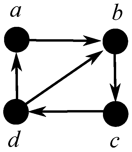
Example 1. 

The directed clique-width of digraph G with vertex set $V\left(G\right)=\{a,b,c,d\}$ and arc set $E\left(G\right)=\left\{\right(a,b),(b,c),(c,d),(d,a),(d,b\left)\right\}$ shown in Figure 1 is at most 3, since it can be defined by the following directed clique-width 3-expression:

$${\alpha }_{3,1}\left({\alpha }_{2,3}(3\left(d\right)\oplus \left({\rho }_{3\to 2}\left({\rho }_{2\to 1}\left({\alpha }_{2,3}(3\left(c\right)\oplus \left({\alpha }_{1,2}(2\left(b\right)\oplus 1\left(a\right))\right))\right)\right)\right))\right)$$

Given a digraph G and an integer k, deciding whether the directed clique-width of G is at most k is NP-complete [17]. In contrast to the undirected case, there are only very few digraph classes for which we know how to compute a directed clique-width expression in polynomial time. This holds for directed co-graphs [5], digraphs of bounded directed modular width [18], and orientations of trees [5]. In order to find directed clique-width expressions for general digraphs one can use results on the related parameter bi-rank-width [19]. By ([15], Lemma 9.9.12) we can use approximate directed clique-width expressions obtained from rank-decomposition with the drawback of a single-exponential blow-up on the parameter.

3. Directed Clique-Width of Minimal Series-Parallel Digraphs (MSP DAGs)

We recall the definition of an MSP DAG which is based on [14] to be the digraph that can be constructed starting from one vertex and recursively using two fundamental operations: series composition and parallel composition.

Definition 2 

(MSP DAG [14]). An MSP DAG is defined recursively as follows:

1. 

A DAG containing only one vertex is an MSP DAG.

2. 

If $G_1$ and $G_2$ are two vertex-disjoint MSP DAGs, then the DAG constructed by each of the following two operations is also an MSP DAG:

(a) 

Parallel composition: $G=G_{1}P{G}_2=(V\left(G_1\right)\cup V\left(G_2\right),E\left(G_1\right)\cup E\left(G_2\right))$.

(b) 

Series composition: $G=G_{1}S{G}_2=(V\left(G_1\right)\cup V\left(G_2\right),E\left(G_1\right)\cup E\left(G_2\right)\cup T_1\times S_2)$ where $T_1$ is the set of sink vertices of $G_1$ and $S_2$ is the set of source vertices of $G_2$.

An MSP DAG G can be represented by a binary decomposition tree $T\left(G\right)$ that reflects the construction of G starting with its vertices using series and parallel operations as follows:

Definition 3 

(Binary decomposition tree of MSP DAGs). The binary decomposition tree $T\left(G\right)$ for an MSP DAG G containing only one vertex v consists of a single node r (the root of T) labeled by v.

The binary decomposition tree $T\left(G\right)$ for an MSP DAG $G=G_{1}P{G}_2$ ($G=G_{1}S{G}_2$) consists of a copy $T_1$ of the binary decomposition tree for $G_1$, a copy $T_2$ of the binary decomposition tree for $G_2$, an additional node r (the root of T) labeled by P (S) and two additional edges between the roots of $T_1$ and $T_2$ and node r. The root of $T_1$ is the left child of r and the root of $T_2$ is the right child of r.

For some node u of $T\left(G\right)$ we define by $G\left[u\right]$ the subgraph of G defined by the subtree of $T\left(G\right)$ rooted at u.

It is proven in [14] that the construction of $T\left(G\right)$ when G is an MSP DAG can be completed in $\mathcal{O}\left(\right|V\left(G\right)|+|E\left(G\right)\left|\right)$ time complexity. This binary decomposition tree of an MSP DAG is the key of defining a directed clique-width expression.

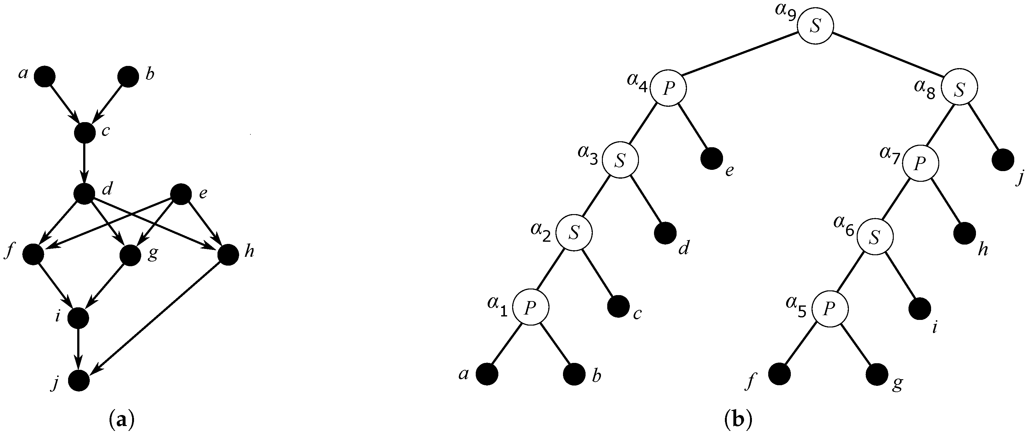
Example 2. 

Figure 2 illustrates an example of an MSP DAG G and its binary decomposition tree $T\left(G\right)$.

Remark 1. 

Since MSP DAGs can define orientations of large complete bipartite graphs the underlying undirected graphs are not $K_4$-minor free graphs. Thus, the underlying undirected graphs of MSP DAGs are not series-parallel graphs. Both graph classes are even incomparable. A more close relation can be shown for the set of edge series-parallel multidigraphs, ESP DAGs for short, which are also defined in [14] from the single arc graph by applying a parallel composition and a series composition. The underlying undirected graph of an ESP DAG is a series-parallel graph. Furthermore, a DAG G with a single source and a single sink is an ESP DAG if and only if its line digraph $LD\left(G\right)$ is an MSP DAG [14].

Notation 1. 

In our directed clique-width expressions, we define an empty expression, denoted by ∅, to be an expression of an empty set of vertices. For any expression t, we consider that $t\oplus \varnothing =t$, so ${\alpha }_{i,j}(t\oplus \varnothing )={\alpha }_{i,j}\left(t\right)$ and ${\rho }_{i\to j}(t\oplus \varnothing )={\rho }_{i\to j}\left(t\right)$.

In [16] it was shown that the directed clique-width of an MSP DAG is at most 7. Next we improve this bound.

Theorem 1. 

Every MSP DAG G has directed clique-width at most 6.

Proof. 

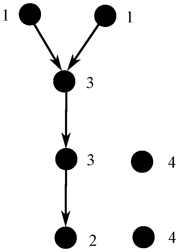
Let G be an MSP DAG and $T\left(G\right)$ be a binary decomposition tree for G. We prove that G has directed clique-width at most 6 by defining a directed clique-width 6-expression for G. We use the 6 labels for the vertices in G as follows (see Figure 3):

• Label 1 is used for the set of non-isolated sources.
• Label 2 is used for the set of non-isolated sinks.
• Label 3 is used for the set of vertices being neither sources nor sinks.
• Label 4 is used for the set of isolated vertices.
• Label 5 is used as an auxiliary label for label 2 for the first graph when we have to distinguish the labels from two combined graphs during the arc insertion operation.
• Label 6 is used as an auxiliary label for label 1 for the second graph when we have to distinguish the labels from two combined graphs during the arc insertion operation.

We define for every node $\alpha$ of $T\left(G\right)$ a directed clique-width 6-expression $t_{\alpha }$ which defines the subgraph $G\left[\alpha \right]$ of G defined by the subtree of $T\left(G\right)$ rooted at $\alpha$ such that all non-isolated sources are labeled by 1, all non-isolated sinks are labeled by 2, all vertices being neither sources nor sinks are labeled by 3, and all isolated vertices are labeled by 4. For every such $t_{\alpha }$ we use two subexpressions $t_{1,\alpha }$ and $t_{2,\alpha }$, such that

• $t_{1,\alpha }$ defines the subgraph of $G\left[\alpha \right]$ given by the non-isolated vertices and
• $t_{2,\alpha }$ defines the subgraph of $G\left[\alpha \right]$ given by isolated vertices.

This allows us to obtain $G\left[\alpha \right]$ by $t_{\alpha }=t_{1,\alpha }\oplus t_{2,\alpha }$.

First, we distinguish between leaf vertices and inner vertices of $T\left(G\right)$:

• Let $\alpha$ be a leaf of $T\left(G\right)$ which represents vertex v of G. We define

  $$\begin{array}{ccc}{t}_{1,\alpha }\hfill & =& \varnothing \hfill \\ t_{2,\alpha }\hfill & =& 4\left(v\right)\hfill \end{array}$$
  For the correctness we note that $t_{\alpha }=t_{1,\alpha }\oplus t_{2,\alpha }$ defines digraph $G\left[\alpha \right]$ and the single isolated vertex is labeled by 4.
• Let $\alpha$ be an internal node of $T\left(G\right)$ and ${\alpha }_1$, ${\alpha }_2$ are respectively the left and right children of $\alpha$. We will construct a directed clique-width 6-expression $t_{\alpha }$ for $G\left[\alpha \right]$ using a directed clique-width 6-expression $t_{{\alpha }_1}$ for $G\left[{\alpha }_1\right]$ and a directed clique-width 6-expression $t_{{\alpha }_2}$ for $G\left[{\alpha }_2\right]$. We can assume that for ${\alpha }_1$ and ${\alpha }_2$ we know the subexpression for the non-isolated and isolated part of $G\left[{\alpha }_1\right]$ and $G\left[{\alpha }_2\right]$, such that

  $$t_{{\alpha }_1}=t_{1,{\alpha }_1}\oplus t_{2,{\alpha }_1}$$

  and

  $$t_{{\alpha }_2}=t_{1,{\alpha }_2}\oplus t_{2,{\alpha }_2}.$$
  To illustrate our following constructions we use two digraphs $G\left[{\alpha }_1\right]$ and $G\left[{\alpha }_2\right]$ in Figure 4a,b. Without loss of generality, and for simplification of reading, we represented in this figure each type of vertex (non-isolated source, non-isolated sink, neither source nor sink, isolated) by a single vertex. The labeling of the vertices using labels from $\{1,\dots ,4\}$ obviously fulfills our given conditions.
  To construct a directed clique-width 6-expression $t_{\alpha }$ for $G\left[\alpha \right]$ we distinguish two cases according to the type of $\alpha$:

  −

  Suppose that $\alpha$ is a P-node. In this case, we define $t_{\alpha }=t_{1,\alpha }\oplus t_{2,\alpha }$, where

  $$\begin{array}{ccc}{t}_{1,\alpha }\hfill & =& t_{1,{\alpha }_1}\oplus t_{1,{\alpha }_2}\hfill \\ t_{2,\alpha }\hfill & =& t_{2,{\alpha }_1}\oplus t_{2,{\alpha }_2}.\hfill \end{array}$$

  Figure 4c illustrates the construction of $G\left[\alpha \right]$ from the two digraphs shown in Figure 4a,b following the expressions $t_{1,\alpha }$ and $t_{2,\alpha }$.

  For the correctness we note that an P-node does not insert any new arcs in the disjoint union of $G\left[{\alpha }_1\right]$ and $G\left[{\alpha }_2\right]$, thus $t_{\alpha }=t_{1,\alpha }\oplus t_{2,\alpha }$ defines the digraph $G\left[\alpha \right]$. Furthermore, by the definition of $t_{\alpha }$ without any relabeling and the assumptions for $t_{{\alpha }_1}$ and $t_{{\alpha }_2}$, in $G\left[\alpha \right]$ all non-isolated sources are labeled by 1, all non-isolated sinks are labeled by 2, all vertices being neither sources nor sinks are labeled by 3, and all isolated vertices are labeled by 4.

  Hence, the expression $t_{\alpha }=t_{1,\alpha }\oplus t_{2,\alpha }$ constructs digraph $G\left[\alpha \right]$ using at most 6 labels.

  −

  Suppose that $\alpha$ is an S-node. In this case, we define $t_{\alpha }=t_{1,\alpha }\oplus t_{2,\alpha }$, where

  $$\begin{array}{ccc}{t}^{\prime }\hfill & =& {\alpha }_{4,2}(t_{2,{\alpha }_1}\oplus {\rho }_{4\to 2}\left(t_{2,{\alpha }_2}\right))\hfill \\ t^{″}\hfill & =& {\alpha }_{5,2}({\rho }_{2\to 5}\left(t_{1,{\alpha }_1}\right)\oplus t^{\prime })\hfill \\ t^{‴}\hfill & =& {\alpha }_{4,6}\left({\alpha }_{5,6}(t^{″}\oplus {\rho }_{1\to 6}\left(t_{1,{\alpha }_2}\right))\right)\hfill \\ t_{1,\alpha }\hfill & =& {\rho }_{6\to 3}\left({\rho }_{5\to 3}\left({\rho }_{4\to 1}\left(t^{‴}\right)\right)\right)\hfill \\ t_{2,\alpha }\hfill & =& \varnothing .\hfill \end{array}$$

  Figure 4d–g illustrate the construction of $G\left[\alpha \right]$ from the two digraphs shown in Figure 4a,b following the expressions $t^{\prime },t^{″},t^{‴},t_{1,\alpha }$, and $t_{2,\alpha }$.

  For the correctness, we observe that $t^{\prime }$ defines the arcs from $t_{2,{\alpha }_1}$ to $t_{2,{\alpha }_2}$, i.e. the arcs between the isolated vertices of $G\left[{\alpha }_1\right]$ to the isolated vertices of $G\left[{\alpha }_2\right]$ using a relabeling from 4 to 2 for those of $G\left[{\alpha }_2\right]$, since they become non-isolated sinks of $G\left[\alpha \right]$. Next $t^{″}$ defines the arcs from $t_{1,{\alpha }_1}$ to $t_{2,{\alpha }_2}$, i.e. the arcs between the non-isolated sinks of $G\left[{\alpha }_1\right]$ and the isolated vertices of $G\left[{\alpha }_2\right]$ are inserted using a relabeling from 2 to auxiliary label 5 for the non-isolated sinks of $G\left[{\alpha }_1\right]$. Further $t^{‴}$ defines the arcs from $t_{1,{\alpha }_1}$ and $t_{2,{\alpha }_1}$ to $t_{1,{\alpha }_2}$, i.e. the arcs from the non-isolated sinks of $G\left[{\alpha }_1\right]$ and the isolated vertices of $G\left[{\alpha }_1\right]$ to the non-isolated sources of $G\left[{\alpha }_2\right]$ using a relabeling from 1 to auxiliary label 6 for the non-isolated sources of $G\left[{\alpha }_2\right]$. Finally in $t_{1,\alpha }$ the relabeling from 4 to 1 ensures that the isolated vertices of $G\left[{\alpha }_1\right]$ are labeled by 1 since they are non-isolated sources in $G\left[\alpha \right]$ and the auxiliary labels 5 and 6 are both changed to 3 since the non-isolated sinks of $G\left[{\alpha }_1\right]$ and the non-isolated sources of $G\left[{\alpha }_2\right]$ are neither sources nor sinks in $G\left[\alpha \right]$. Expression $t_{2,\alpha }$ is empty, since $G\left[\alpha \right]$ does not contain isolated vertices.

  Hence, the expression $t_{\alpha }=t_{1,\alpha }\oplus t_{2,\alpha }$ constructs digraph $G\left[\alpha \right]$ using at most 6 labels.

By traversing $T\left(G\right)$ in post-order we can calculate a directed clique-width 6-expression $t_{\alpha }$ for every node $\alpha$ of $T\left(G\right)$ by the expressions given above. Since the r root of $T\left(G\right)$ represents to whole digraph G we know that G can be constructed by directed clique-width 6-expression $t_r$ and thus has directed clique-width at most 6.    □

The construction of an MSP DAG by a directed clique-width 6-expression described in the proof of Theorem 1 can be translated into a pseudo code shown in Algorithm 1. Our algorithm associates with every node $\alpha$ of $T\left(G\right)$ two expressions $t_1\left(\alpha \right)$ and $t_2\left(\alpha \right)$, where $t_1\left(\alpha \right)$ represents the construction of the subgraph induced by the non-isolated vertices of $G\left[\alpha \right]$ and $t_2\left(\alpha \right)$ represents the construction of the subgraph induced by the isolated vertices of $G\left[\alpha \right]$. At most one of the expressions $t_1\left(\alpha \right)$ and $t_2\left(\alpha \right)$ may be empty. The labels at the end of the computation of $t_1\left(\alpha \right)$ or $t_2\left(\alpha \right)$ represent implicitly whether the corresponding vertices are non-isolated sources (labeled by 1), non-isolated sinks (labeled by 2), vertices that are not sources and not sinks (labeled by 3), or isolated vertices (labeled by 4) in $G\left[\alpha \right]$. Initially, in Step 3, every vertex is labeled by 4 since the subgraph induced by a leaf of $T\left(G\right)$ consists only of one isolated vertex. Step 5 determines the left child ${\alpha }_1$ and the right child ${\alpha }_2$ of an internal node $\alpha$. Steps 7 and 8 construct the expression $t_1\left(\alpha \right)$ and $t_2\left(\alpha \right)$ for a P-node $\alpha$ to be respectively the disjoint union of $t_1\left({\alpha }_1\right),t_1\left({\alpha }_2\right)$ and the disjoint union of $t_2\left({\alpha }_1\right),t_2\left({\alpha }_2\right)$. Steps 10–14 construct the expressions $t_1\left(\alpha \right)$ and $t_2\left(\alpha \right)$ for an S-node $\alpha$ as follows: Step 10 changes the label of isolated vertices of $G\left[{\alpha }_2\right]$ from 4 to 2 and inserts all arcs from an isolated vertex of $G\left[{\alpha }_1\right]$ to an isolated vertex of $G\left[{\alpha }_2\right]$; Step 11 changes the label of non-isolated sinks of $G\left[{\alpha }_1\right]$ from 2 to (auxiliary label) 5 and inserts all arcs from a non-isolated sink of $G\left[{\alpha }_1\right]$ to an isolated vertex of $G\left[{\alpha }_2\right]$; Step 12, changes the label of non-isolated sources of $G\left[{\alpha }_2\right]$ from 1 to (auxiliary label) 6 and inserts all arcs from an isolated vertex of $G\left[{\alpha }_1\right]$ to a non-isolated source of $G\left[{\alpha }_2\right]$ and all arcs from a non-isolated sink of $G\left[{\alpha }_1\right]$ to a non-isolated source of $G\left[{\alpha }_2\right]$. Step 13, changes the label of every isolated vertex of $G\left[{\alpha }_1\right]$ from 4 to 1 since these vertices are non-isolated sources in $G\left[\alpha \right]$, changes the label of every non-isolated sink of $G\left[{\alpha }_1\right]$ from 5 to 3, since these vertices are neither sources nor sinks in $G\left[\alpha \right]$, and changes the label of every non-isolated source of $G\left[{\alpha }_2\right]$ from 6 to 3, since these vertices are also neither sources nor sinks in $G\left[\alpha \right]$. The expression $t_2\left(\alpha \right)$ must be empty because of $G\left[\alpha \right]$ is connected. Since the number of nodes in $T\left(G\right)$ is $\mathcal{O}\left(n\right)$ and every step can be done in $\mathcal{O}\left(1\right)$ time, the total time complexity of Algorithm 1 is in $\mathcal{O}\left(n\right)$.

Corollary 1. 

For every MSP DAG G which is given by its binary decomposition tree $T\left(G\right)$ a directed clique-width 6-expression can be found in time $\mathcal{O}\left(\right|V\left(G\right)\left|\right)$.

Algorithm 1 Construction directed clique-width 6-expression of an MSP DAG
	Input A binary decomposition tree $T\left(G\right)$ of an MSP DAG G. Output A directed clique-width 6-expression of G. Let $\alpha$ be a node on a post-order traversal of $T\left(G\right)$.
1:	if  $\alpha$ is a leaf representing vertex v then
2:	$t_1\left(\alpha \right)=\varnothing$
3:	$t_2\left(\alpha \right)=4\left(v\right)$
4:	else
5:	let ${\alpha }_1$ and ${\alpha }_2$ be respectively the left and right children of $\alpha$
6:	if $\alpha$ is a P-node then
7:	$t_1\left(\alpha \right)=t_1\left({\alpha }_1\right)\oplus t_1\left({\alpha }_2\right)$
8:	$t_2\left(\alpha \right)=t_2\left({\alpha }_1\right)\oplus t_2\left({\alpha }_2\right)$
9:	else	▹$\alpha$ is an S-node
10:	$E_1={\alpha }_{4,2}(t_2\left({\alpha }_1\right)\oplus {\rho }_{4\to 2}\left(t_2\left({\alpha }_2\right)\right))$	▹ arcs from $t_2\left({\alpha }_1\right)$ to $t_2\left({\alpha }_2\right)$
11:	$E_2={\alpha }_{5,2}({\rho }_{2\to 5}\left(t_1\left({\alpha }_1\right)\right)\oplus E_1)$	▹ arcs from $t_1\left({\alpha }_1\right)$ to $t_2\left({\alpha }_2\right)$
12:	$E_3={\alpha }_{4,6}\left({\alpha }_{5,6}(E_2\oplus {\rho }_{1\to 6}\left(t_1\left({\alpha }_2\right)\right))\right)$	▹ arcs from $t_1\left({\alpha }_1\right)$ and $t_2\left({\alpha }_1\right)$ to $t_1\left({\alpha }_2\right)$
13:	$t_1\left(\alpha \right)={\rho }_{6\to 3}\left({\rho }_{5\to 3}\left({\rho }_{4\to 1}\left(E_3\right)\right)\right)$	▹ relabeling
14:	$t_2\left(\alpha \right)=\varnothing$

Example 3. 

Figure 5 illustrates the application of Algorithm 1 for the digraph G and its binary decomposition tree $T\left(G\right)$ shown in Figure 2. The inner nodes are visited according to a post-order traversal of $T\left(G\right)$ which is defined by the symbols ${\alpha }_i$, $1\le i\le 9$, written near every internal node of $T\left(G\right)$. Every subfigure in Figure 5 shows a digraph $G\left[{\alpha }_i\right]$, $1\le i\le 9$, defined by expression $t_1\left({\alpha }_i\right)\oplus t_2\left({\alpha }_i\right)$ of Algorithm 1. Digraph $G\left[{\alpha }_9\right]$ obviously corresponds to digraph G.

Remark 2. 

A useful property of Algorithm 1 is that the number of relabelings of the vertices is bounded. A relabeling of a vertex is done if and only if the state (non-isolated source, non-isolated sink, neither source nor sink, isolated) of the vertex is changed. Since the state of a vertex can change at most twice and an auxiliary label 5 or 6 is given at most once to every vertex, every vertex changes its label at most three times.

The problem of finding a decomposition tree $T\left(G\right)$ for some special graph G in polynomial time is a well studied problem. For every MSP DAG and also for every directed co-graph, a decomposition tree can be found in linear time [14,20]. The reverse direction, i.e. constructing G in linear time from $T\left(G\right)$ seems to be unsolved for MSP DAGs. Our shown 6-expression allows to solve this problem.

Corollary 2. 

Every MSP DAG G can be constructed from its binary decomposition tree $T\left(G\right)$ in time $\mathcal{O}\left(\right|V\left(G\right)|+|E\left(G\right)\left|\right)$.

Proof. 

Let $T\left(G\right)$ a binary decomposition tree for some MSP DAG G. By Corollary 1 from $T\left(G\right)$ we can define a directed clique-width 6-expression X for G in time $\mathcal{O}\left(\right|V\left(G\right)\left|\right)$.

In order to access vertices of a given label i we maintain in each node u of the 6-expression-tree (see Section 4) for X an array containing at i a pointer to a list of the vertices of label i in the digraph defined by subtree with root u for $1\le i\le 6$. Our expression X only inserts new arcs, such that these operations use time $\mathcal{O}\left(\right|E\left(G\right)\left|\right)$ and by Remark 2, the number of relabelings is at most three for every vertex. Thus, G can be constructed from $T\left(G\right)$ in time $\mathcal{O}\left(\right|V\left(G\right)|+|E\left(G\right)\left|\right)$. □

4. Algorithmic Consequences

By the given definition every graph of directed clique-width at most k can be represented by a tree structure, denoted as k-expression-tree. The leaves of the k-expression-tree represent the vertices of the digraph and the inner nodes of the k-expression-tree correspond to the operations applied to the subexpressions defined by the subtrees. Using the k-expression-tree many hard problems have been shown to be solvable in polynomial time when restricted to graphs of bounded directed clique-width [4,5].

In order to show tractability for several digraph problems w.r.t. the parameter directed clique-width one can use its defineability within monadic second order logic (MSO). We restrict to ${\mathrm{MSO}}_1$-logic, which allows propositional logic, variables for vertices and vertex sets of digraphs, the predicate $\mathrm{arc}(u,v)$ for arcs of digraphs, and quantifications over vertices and vertex sets [21]. For defining optimization problems we refer to the ${\mathrm{LinEMSO}}_1$ framework given in [2].

In several papers (cf. [4,19,22]) it has been shown, that all digraph problems expressible in monadic second order logic with quantifications over vertices and vertex sets (${\mathrm{MSO}}_1$-logic) are fixed parameter tractable with respect to the parameter “directed clique-width of the input graph”. Theorem 1 leads to the next result.

Corollary 3. 

Every digraph problem expressible in ${\mathit{MSO}}_1$-logic can be solved in polynomial time on MSP DAGs.

Examples for problems expressible in ${\mathrm{MSO}}_1$-logic are the directed vertex disjoint paths problem [4] and also the arc disjoint paths problem [23].

Corollary 4. 

The directed vertex disjoint paths problem and the arc disjoint paths problem can be solved in polynomial time on MSP DAGs.

There are a lot of further problems which can be solved efficiently on graphs of bounded directed clique-width. This follows by the xp-algorithms for the problems directed Hamiltonian path, directed Hamiltonian cycle, directed cut, and regular subdigraph with respect to the parameter directed NLC-width given in [5].

Corollary 5. 

The directed Hamiltonian path problem, directed Hamiltonian cycle problem, directed cut problem, and regular subdigraph problem can be solved in polynomial time on MSP DAGs.

5. Conclusions and Outlook

We have given an improved upper bound for the directed clique-width of MSP DAGs. Since the directed clique-width occurs in the exponent of the runtimes of algorithms for interesting problems our result improves the runtime of several algorithms on MSP DAGs. Further our findings extend the few known results on digraph classes with bounded directed clique-width.

It remains to show that the improved upper bound of 6 for the directed clique-width of MSP DAGs is tight. This might be done by further characterizations of MSP DAGs or using a computer program.

In our future work we also want to analyze the structure, relation, and directed clique-width of digraph classes obtained by slight modifications of the series operation considered in this paper. Among these are connecting every source of the first digraph with every sink of the second digraph (MSP-ST DAGs, ([24], Definition 2)), connecting every source of the first digraph with every source of the second digraph (MSP-SS DAGs, ([24], Definition 5)), and connecting every sink of the first digraph with every sink of the second digraph (MSP-TT DAGs, ([24], Definition 8)).

Further, we want to analyze whether the recursive structure of MSP DAGs and the similar classes mentioned above can be used to give linear time solutions for the directed vertex disjoint paths problem and the arc disjoint paths problem in order to improve our results of Corollary 4.

As mentioned in Remark 1 the class of edge series-parallel multidigraphs defined in [14] leads to a specific orientation of (undirected) series-parallel graphs and seems also to be interesting for our further research on digraph classes on bounded directed clique-width.

Finally, in [14] only oriented graphs are considered. Therefore we want to analyze series operations which also define both possible directed edges between two vertices, i.e., so-called symmetric arcs.