General Position Subset Selection in Line Arrangements ^†

Abstract

Given a set of n points in a plane, the General Position Subset Selection problem is that of finding a maximum-size subset of points in general position, i.e., with no three points collinear. The problem is known to be hard computationally, and the best approximation ratio known is $\mathrm{\Omega }\left(n^{-1/2}\right)$. Here, we obtain better approximations in three special cases: (I) a constant-factor approximation for the case where the input set consists of lattice points and is dense, which means that the ratio between the maximum and the minimum distance in P is of the order of $\mathrm{\Theta }\left(\sqrt{n}\right)$; (II) an $\mathrm{\Omega }\left({(logn)}^{-1/2}\right)$-approximation for the case where the input set is the set of vertices of a generic n-line arrangement, i.e., one with $\mathrm{\Omega }\left(n^2\right)$ vertices; and (III) an $\mathrm{\Omega }\left({(logn)}^{-1/2}\right)$-approximation for the case where the input set has at most $O\left(\sqrt{n}\right)$ points collinear and can be covered by $O\left(\sqrt{n}\right)$ lines. The scenario in (I) is a special case of that in (II). Our approximations rely on probabilistic methods and results from incidence geometry.

1. Introduction

A set of points in the plane is said to be in general position if no three points are collinear. The problem of selecting a large subset of points from a $k\times k$ grid of integer points with no three points collinear (i.e., in general position) goes back more than 100 years; see, for example, [1,2] (Ch. 10). In particular, it is not known if one can always select $2k$ points from the $k\times k$ grid so that no three points are collinear [1].

A key quantity in the process of selecting a large subset from an input set of points is the number of collinear triples in the set. Payne and Wood [3] obtained the following upper bound on this number. The proof relies on the classical points and line incidence bound due to Szemerédi and Trotter [4]; see also [5] (Chap. 10) and [6] for a modern approach to this topic. The special case $\ell =O\left(\sqrt{n}\right)$ in the lemma can also be found in [7] or in [8] (p. 313).

Lemma 1

([3]). Let P be a set of n points in the plane with at most ℓ collinear. Then, the number of collinear triples in P is $T=O(n^{2}log\ell +{\ell }^{2}n)$. In particular, if $\ell =O\left(\sqrt{n}\right)$, then $T=O(n^{2}log\ell )$.

By applying the above lemma together with a lower bound on the independence number of a hypergraph obtained by Spencer [9], Payne and Wood [3] obtained the following result.

Theorem 1

([3]). Let P be a set of n points in the plane with at most ℓ collinear. Then, P contains a subset of $\mathrm{\Omega }\left(n/\sqrt{nlog\ell +{\ell }^2}\right)$ points in general position. In particular, if $\ell =O\left(\sqrt{n}\right)$, then P contains a subset of $\mathrm{\Omega }\left({(n/log\ell )}^{1/2}\right)$ points in general position.

A cursory examination of the above lower bound shows that if the input set has a large subset of points in general position (of, say, nearly linear size), then the above guarantee is roughly a factor of $\sqrt{n}$ smaller than the truth.

Given a set P of points in the plane, the General Position Subset Selection problem (GPSS, for short), is that of finding a maximum-size subset of points in general position. The problem is known to be NP-complete and APX-hard, and the current best approximation for the problem is a greedy algorithm due to Cao [10] (Chap. 3), achieving a ratio of $\mathrm{\Omega }\left({\mathsf{OPT}}^{-1/2}\right)=\mathrm{\Omega }\left(n^{-1/2}\right)$; here, $\mathsf{OPT}$ is the cardinality of an optimum solution to GPSS. See also [11] (Chap. 9) and [12] for further aspects of this problem and [13] for basic notions in complexity and approximation. Throughout this paper, $\mathsf{ALG}$ denotes the cardinality of the solution to GPSS computed by an algorithm under consideration.

As in [13], here, we follow the convention that the approximation ratio of an algorithm for a maximization problem is less than 1. Throughout this paper, all logarithms are in base 2.

• Our results.

(I) For a set P of n points in the plane, consider the ratio (sometimes also called spread)

$$D\left(P\right)={\displaystyle \frac{max\left\{\right|ab|:a,b\in P,a\ne b\}}{min\left\{\right|ab|:a,b\in P,a\ne b\}}},$$

where $\left|ab\right|$ is the Euclidean distance between points a and b. Since the general position property is unaffected by scaling, we may assume, without loss of generality, that $min\left\{\right|ab|:a,b\in P,a\ne b\}=1$. In this case, $D\left(P\right)=max\left\{\right|ab|:a,b\in P,a\ne b\}$ is the diameter of P. A standard disk packing argument shows that if $\left|P\right|=n$, then $D\left(P\right)\ge {\alpha }_0{n}^{1/2}$, where

$${\alpha }_0:=2^{1/2}{3}^{1/4}{\pi }^{-1/2}\approx 1.05,$$

(1)

provided that n is large enough; see [14] (Prop. 4.10). On the other hand, a $\sqrt{n}\times \sqrt{n}$ section of the integer lattice shows that this bound is tight up to a constant factor. An n-element point set P satisfying the condition $D\left(P\right)\le \alpha n^{1/2}$, for some constant $\alpha \ge {\alpha }_0$, is said to be $\alpha$-dense; see, for instance, [15] and Figure 1 for an illustration.

We obtain a constant-factor approximation for GPSS in dense lattice point sets; its approximation ratio depends on the spread ratio of the input.

Theorem 2.

Given an α-dense set of n lattice points, an $\mathrm{\Omega }\left({\alpha }^{-2}\right)$-approximation for the General Position Subset Selection problem can be computed in polynomial time.

(II) According to a classical result of Beck [16], if P is a set of n points in the plane with at most ℓ points collinear, then P determines at least $\mathrm{\Omega }\left(n\right(n-\ell \left)\right)$ distinct lines. In particular, if $\ell \le cn$, where $c<1$ is a constant, then P determines $\mathrm{\Omega }\left(n^2\right)$ distinct lines. By duality (see, e.g., [17]), for a set L of n lines in the plane, where at most ℓ lines of L are concurrent, the number of vertices of the corresponding arrangement is $\mathrm{\Omega }\left(n\right(n-\ell \left)\right)$. We say that an arrangement of n lines is generic if it has $\mathrm{\Omega }\left(n^2\right)$ vertices.

We obtain an $\mathrm{\Omega }\left({(logn)}^{-1/2}\right)$-approximation for GPSS in the special case where the input set is the set of vertices of an n-line arrangement under the relatively mild genericity assumption.

Theorem 3.

Given n lines in the plane that make a generic line arrangement, an $\mathrm{\Omega }\left({(logn)}^{-1/2}\right)$-approximation for the General Position Subset Selection problem for the set of vertices of the corresponding line arrangement can be computed using a randomized algorithm in expected polynomial time.

Essentially, the same proof (of this theorem in Section 3) yields the following.

Corollary 1.

Given n lines in the plane, let V denote the vertex set of the corresponding line arrangement. If $V^{\prime }\subseteq V$ is a subset of vertices with $|V^{\prime }| =\mathrm{\Omega }\left(n^2\right)$, an $\mathrm{\Omega }\left({(logn)}^{-1/2}\right)$-approximation for the General Position Subset Selection problem in $V^{\prime }$ can be computed using a randomized algorithm in expected polynomial time.

It is worth noting that the scenario in Theorem 2 is a special case of the scenario in Theorem 3. Indeed, any finite set P of lattice points in the integer grid is a subset of the vertices of an arrangement ${\mathrm{A}}^{+}$ of axis-parallel lines induced by H and V, the sets of horizontal and vertical lines incident to points in P, respectively. Moreover, if P is a dense set, then ${\mathrm{A}}^{+}$ is generic, since

$$\left|H\right|,\left|V\right|=\mathrm{\Omega }\left(\right|P|/\left(\alpha \sqrt{n}\right)) =\mathrm{\Omega }\left(\sqrt{n}\right),$$

Thus, ${\mathrm{A}}^{+}$ has $\left|H\right|·\left|V\right|=\mathrm{\Omega }\left(n\right)$ vertices. Observe that not all vertices in the arrangement ${\mathrm{A}}^{+}$ are necessarily in P.

(III) Given a set P of points in the plane, a line cover of P is a set of lines that cover all points in P. Computing a line cover of minimum size is APX-hard, and the best approximation ratio known is $O(logn)$ [18].

We obtain an $\mathrm{\Omega }\left({(logn)}^{-1/2}\right)$-approximation for GPSS in the special case where the input set has at most $O\left(\sqrt{n}\right)$ points collinear and can be covered by $O\left(\sqrt{n}\right)$ lines.

Theorem 4.

Given a set P of n points in the plane with at most $O\left(\sqrt{n}\right)$ collinear and with a line cover of size $O\left(\sqrt{n}\right)$, an $\mathrm{\Omega }\left({(logn)}^{-1/2}\right)$-approximation for the General Position Subset Selection problem can be computed using a randomized algorithm in expected polynomial time.

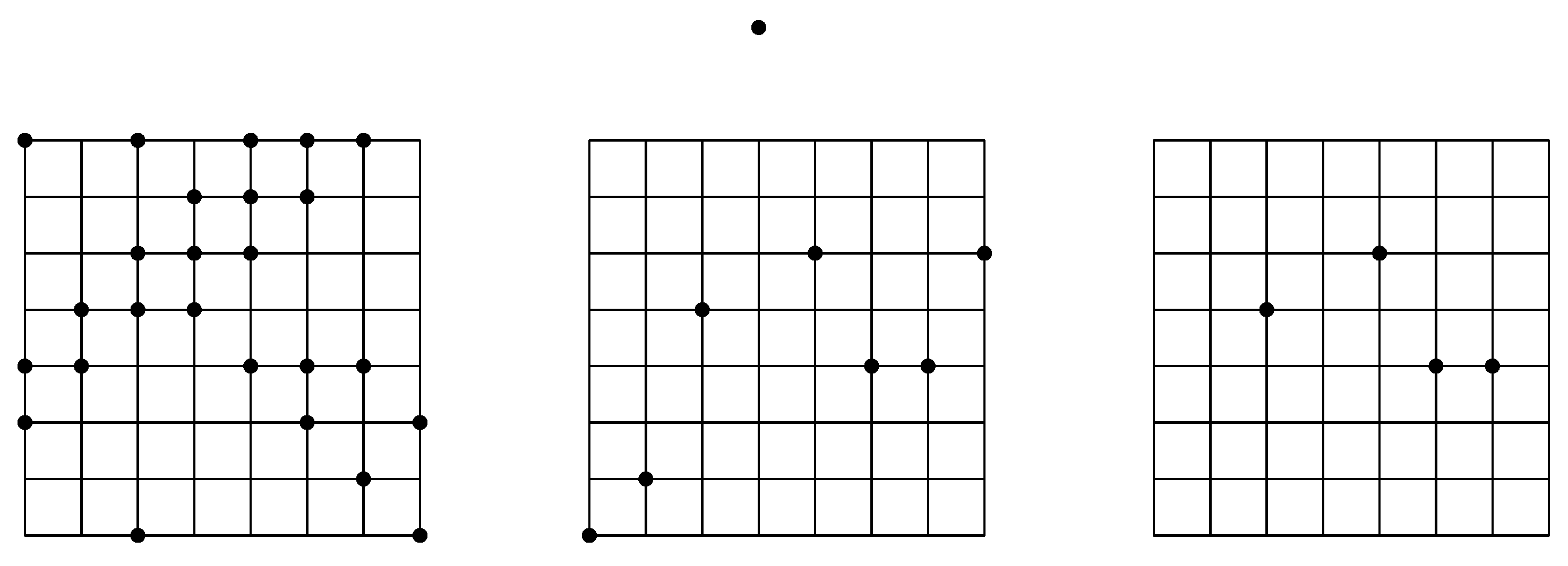
2. Subset Selection in Dense Lattice Point Sets

In this section, we prove Theorem 2. First, we introduce the setup.

For a positive integer m, the $m\times m$ grid is the set of points in the plane $G_m=\{(x,y):x,y\in \{0,1,\dots ,m-1\}$. We have $|G_m| =m^2$. Following [19], let $k\left(m\right)$ denote the minimum number of colors in a coloring of the points in $G_m$ such that no three collinear points are monochromatic. Since no three points in a single row or column can receive the same color, we have $k\left(m\right)\ge m/2$. It was shown by Wood [19] that for any $\epsilon >0$, $k\left(m\right)\le (2+\epsilon )m$ for every $m\ge M\left(\epsilon \right)$. Among other facts, this is based on the fact that for any $\epsilon >0$, there exists a prime between m and $(1+\epsilon )m$, for every $m\ge M\left(\epsilon \right)$. A non-asymptotic result, more convenient for small m, is that there exists a prime between m and $6m/5$, for every $m\ge 25$ [20]. (And by the well-known Bertrand–Chebyshev theorem, there exists a prime between m and $2m$, for every m.)

We briefly recall Wood’s argument [19] relying on a construction of Erdos [21]. Let $p\ge m$ be a prime; in practice we may pick the smallest prime at least m or a prime at least m that is close to m. For any integer i, let

$$V_i=\{(x,(x^{2}modp)+i):x=0,1,\dots ,m-1\}.$$

Note that $|V_i| =m$, and that $V_i$ may be not contained in $G_m$; refer to Figure 1. A Vandermonde determinant calculation shows that $V_i$ is in general position for every $i\in \mathbb{Z}$. Moreover, $V_i\cap V_j=\varnothing$ whenever $i\ne j$. Each point $(x,y)\in G_m$ is in $V_i$, where $i=y-(x^{2}modp)$. Since

$$1-p=0-(p-1)\le y-(x^{2}modp)\le m-1,$$

the union of the $m+p-1$ sets $V_i$ over $i=1-p,\dots ,m-1$ consists of $m+p-1$ color classes, where each class is in general position. That is, $G_m$ can be covered by $m+p-1$m-element point sets in general position. As mentioned in the previous paragraph, $m+p-1\le (2+\epsilon )m$ for every $m\ge M\left(\epsilon \right)$, or $m+p-1\le 11m/5$ for every $m\ge 25$, as needed.

Proof of Theorem 2.

Since P is $\alpha$-dense, we may assume that $P\subseteq G_m$, where $m=\lceil \alpha \sqrt{n}\rceil$, after a suitable translation with an integer vector. The algorithm chooses a prime $p\ge m$ close to m. Recall that primality testing can be realized in polynomial time, that is, in $O\left({log}^{O\left(1\right)}m\right)$ time; see, e.g., [22] or [23] (Ch. 14.6). By the Prime Number Theorem, finding a prime $p\ge m$ close to m involves the primality testing of $O\left(m^{0.525}\right)=O\left(n^{0.263}\right)$ odd integers in the interval $[m,m+2m^{0.525}]$ [24].

As argued above, $G_m$ is covered by $m+p-1\le (2+\epsilon )m$m-element point sets $V_i$ in general position. By monotonicity (i.e., every subset of a set in general position is likewise in general position), the sets $P\cap V_i$ are in general position, and the algorithm outputs the largest one, with at least ${\displaystyle \frac{n}{(2+\epsilon )m}}$ elements.

Since each of the m rows of $G_m$ contains at most two elements of an optimal solution, we have $\mathsf{OPT}\le 2m$. Consequently, the ratio $\mathsf{ALG}/\mathsf{OPT}$ is bounded from below as

$${\displaystyle \frac{\mathsf{ALG}}{\mathsf{OPT}}}\ge {\displaystyle \frac{n}{2·(2+\epsilon )m^2}}=\mathrm{\Omega }\left({\displaystyle \frac{1}{{\alpha }^2}}\right).$$

The approximation ratio in the formula is roughly $1/\left(4{\alpha }^2\right)$, for a small $\epsilon$. Clearly, the resulting algorithm runs in polynomial time: choosing the prime p and generating the sets $V_i$ takes $O\left(n\right)$ time. Selecting one $V_i$ with a maximal size $|P\cap V_i|$ can be achieved within the same time, and so the overall running time is $O\left(n\right)$. □

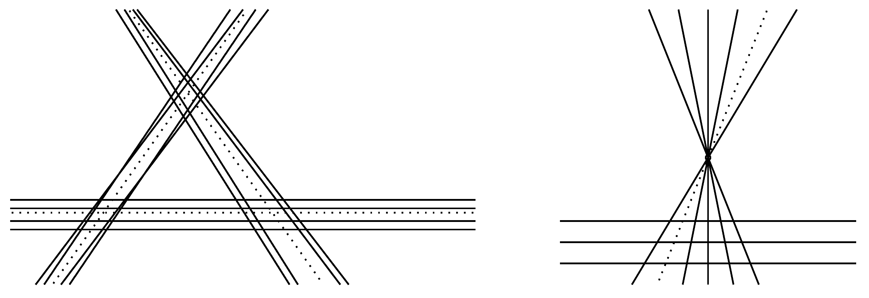
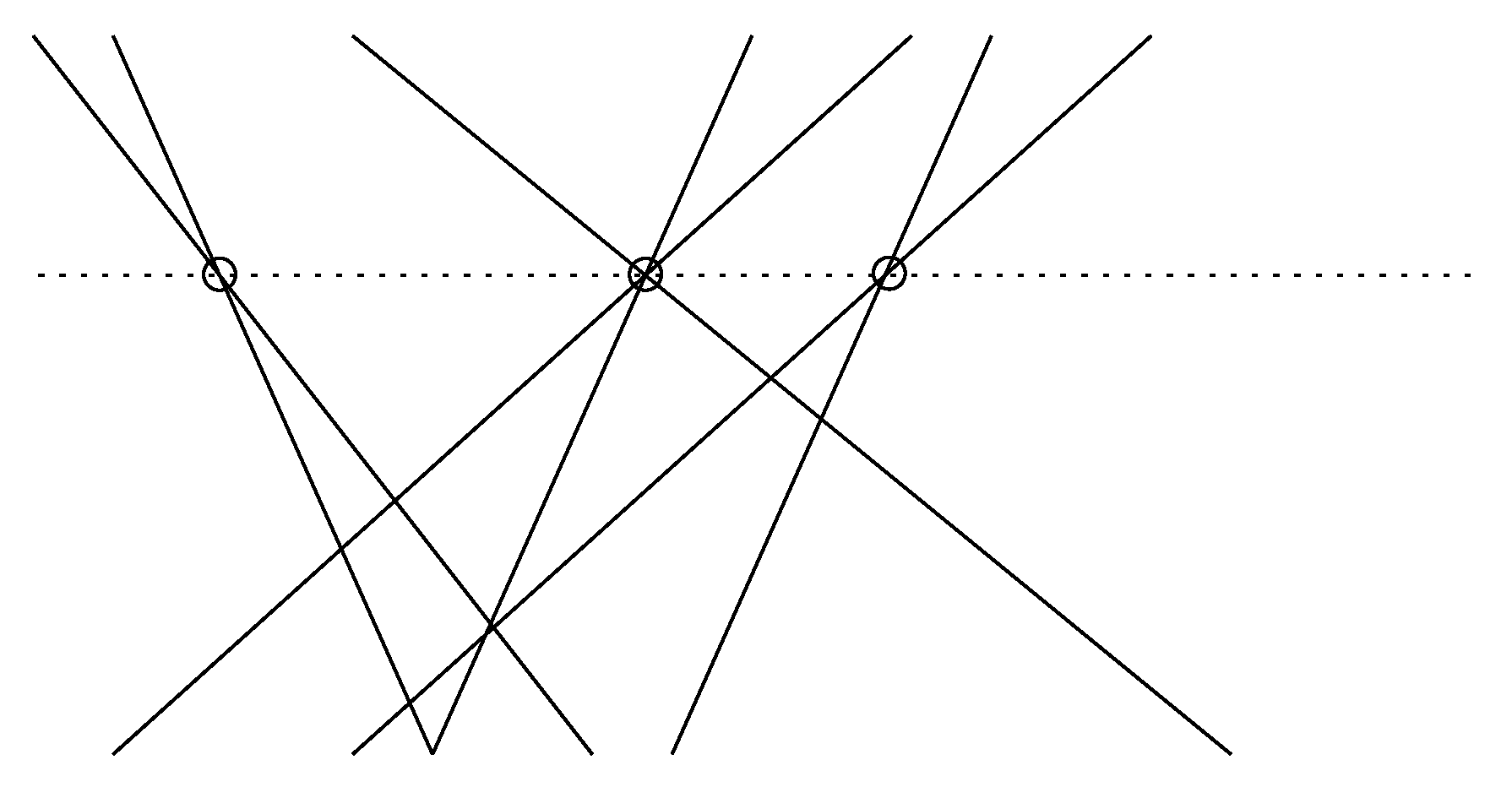
3. Subset Selection in Generic Line Arrangements

In this section, we prove Theorem 3. Recall that an arrangement of n lines is generic if it has $\mathrm{\Omega }\left(n^2\right)$ vertices. See Figure 2.

Lemma 2.

Let V be the set of vertices of an n line arrangement $=\left(L\right)$, where $L=\{{\ell }_1,\dots ,{\ell }_n\}$. Then, $\ell \left(V\right)\le n-1$.

Proof. 

We distinguish two cases. Let $V^{\prime }\subseteq V$ be a set of collinear vertices, say on a line h. If $h\in L$, then obviously $|V^{\prime }|\le n-1$. If $h\notin L$, scan h, say, from left to right, and observe that each vertex in $V^{\prime }$ uses up at least two “new” lines from L; thus, $|V^{\prime }| \le n/2$. See Figure 3. □

Let V be the set of vertices of a generic n line arrangement $=\left(L\right)$. Let $N=\left|V\right|\le \left({\displaystyle \genfrac{}{}{0pt}{}{n}{2}}\right)$; we also have $N\ge c{n}^2$ by the assumption. By Lemma 2, $\ell :=\ell \left(V\right)\le n-1$; thus, by Lemma 1, the number of collinear triples is bounded as

$$\begin{array}{cc}\hfill T& =O(N^{2}log\ell +{\ell }^{2}N)=O(N^{2}logn+n^{2}N).\hfill \end{array}$$

(2)

Proof of Theorem 3.

The subset selection algorithm consists of two steps: (i) random sampling from V and (ii) the application of the deletion method. See, e.g., [25] (Chap. 3) and a similar application in [26]. In the first step, a random subset $X\subset V$ is chosen by selecting points independently with probability $p=k/N$, for a suitable k to be determined. Note that $\mathrm{E}\left[\right|X\left|\right]=N·k/N=k$.

To select a subset in general position, one needs to avoid one type of obstacle, collinear triples. One obstacle can be eliminated by deleting one point from each surviving collinear triple in the second step. In particular, it suffices to choose k so that

$$\mathrm{E}\left[T{p}^3\right]\le k/2,$$

since this implies that the expected number of remaining points is at least $k-k/2=k/2$. Let $c_1$ denote the constant hidden in (2). With the previous upper bound on T, and recalling that $N\ge c{n}^2$, it suffices to choose k so that

$$2c_1{k}^2(Nlogn+n^2)\le N^2.$$

(3)

Setting $k=c^{\prime }{\displaystyle \frac{n}{\sqrt{logn}}}$ for a sufficiently small $c^{\prime }>0$ satisfies the inequality, proving the lower bound on the size of the output. In addition, this setting is valid for ensuring that $p=k/N<1$.

In summary, the expected number of points in general position found using the algorithm is $\mathrm{\Omega }\left({\displaystyle \frac{n}{\sqrt{logn}}}\right)$. To analyze the approximation ratio, it suffices to notice that $\mathsf{OPT}\le 2n$. Indeed, for each line ${\ell }_i\in L$, $i=1,\dots ,n$, at most two vertices in V can appear in any solution; thus, $\mathsf{OPT}\le 2n$. It follows that the approximation ratio is

$${\displaystyle \frac{\mathsf{ALG}}{\mathsf{OPT}}}={\displaystyle \frac{1}{2n}}·\mathrm{\Omega }\left({\displaystyle \frac{n}{\sqrt{logn}}}\right)=\mathrm{\Omega }\left({\displaystyle \frac{1}{\sqrt{logn}}}\right),$$

as claimed.

Since repeated random samplings are independent, the probability of error for the resulting randomized algorithm of not finding the required number of points can be made arbitrarily small by repetition—in standard fashion. Clearly, the resulting algorithm runs in expected polynomial time; we give a few details below.

Computing the set of vertices V and performing the random sampling takes $O\left(n^2\right)$ time. The expected sample size is $O\left(k\right)=O\left(n\right)$. Using the point–line duality, the algorithm computes the line arrangement dual to the point sample in $O\left(n^2\right)$ time [27] (Ch. 8). It repeatedly removes lines passing through vertices incident to at least three lines, each in $O\left(n\right)$ time, and updates the line arrangement. This step is repeated until the arrangement is simple, and thus, the points left in the sample are in general position. The expected running time is $O\left(n^2\right)$. □

Proof of Corollary 1.

We perform random sampling from $V^{\prime }$, let $N= |V^{\prime }|$, and proceed as in the proof of Theorem 3. Inequality (3) is again satisfied due to the assumption $|V^{\prime }| =\mathrm{\Omega }\left(n^2\right)$. □

4. Another Application

In this section, we restrict ourselves to General Position Subset Selection in grid-like sets, that is, sets with at most $\ell =O\left(\sqrt{n}\right)$ points collinear and with a line cover of size $\kappa =O\left(\sqrt{n}\right)$. The approximation is obtained with an approach similar to that in the proof of Theorem 3.

Proof of Theorem 4.

By the first assumption and Lemma 1, the number of collinear triples in P is

$$T=O(n^{2}log\ell )=O(n^{2}logn).$$

(4)

Since an optimal solution can contain at most two points of P from each line in an optimal line cover of P, we have $\mathsf{OPT}\le 2\kappa =O\left(\sqrt{n}\right)$. The subset selection algorithm consists of two steps: (i) random sampling from P and (ii) the application of the deletion method. In the first step, a random subset $X\subset P$ is chosen by selecting points independently with probability $p=k/n$, for a suitable k to be determined. Note that $\mathrm{E}\left[\right|X\left|\right]=n·k/n=k$.

As in the proof of Theorem 3, it suffices to choose k so that

$$\mathrm{E}\left[T{p}^3\right]\le k/2.$$

Let $c_1$ denote the constant hidden in (4). Using the upper bound on T in (4), it suffices to choose k so that

$$2c_1{k}^{2}logn\le n.$$

(5)

Setting $k=c^{\prime }\sqrt{{\displaystyle \frac{n}{logn}}}$ for a sufficiently small $c^{\prime }>0$ satisfies the inequality, proving the lower bound on the size of the output. In addition, this setting is valid for ensuring that $p=k/n<1$.

The expected number of points in general position found using the algorithm is $\mathrm{\Omega }\left(\sqrt{{\displaystyle \frac{n}{logn}}}\right)$. By recalling that $\mathsf{OPT}\le 2\kappa =O\left(\sqrt{n}\right)$, it follows that the approximation ratio is

$${\displaystyle \frac{\mathsf{ALG}}{\mathsf{OPT}}}\ge {\displaystyle \frac{1}{2\kappa }}·\mathrm{\Omega }\left(\sqrt{{\displaystyle \frac{n}{logn}}}\right)=\mathrm{\Omega }\left({\displaystyle \frac{1}{\sqrt{logn}}}\right),$$

as claimed. □

5. Concluding Remarks

We conclude with some problems for further investigation:

• Can the approximation factor in Theorem 3 be improved? Perhaps using ideas from [28] (Section 2)?
• Is there a constant-factor approximation for GPSS among the vertices of an n-line arrangement?
• Can a constant-factor approximation for GPSS on point sets satisfying $\ell =O\left(\sqrt{n}\right)$ and $\kappa =O\left(\sqrt{n}\right)$ be obtained? Note that one can select $\mathrm{\Theta }\left(\sqrt{n}\right)$ points in general position from the $\sqrt{n}\times \sqrt{n}$ grid of n points; see, e.g., refs. [25] (Ch. 3.3) or [2] (Ch. 10).
• Can better approximation factors for the general position subset selection problem be obtained in other interesting scenarios?

References

1. Dudeney, H. A puzzle with pawns. In Amusements in Mathematics; Nelson: Edinburgh, UK, 1917; p. 94. [Google Scholar]
2. Braß, P.; Moser, W.; Pach, J. Research Problems in Discrete Geometry; Springer: New York, NY, USA, 2005. [Google Scholar]
3. Payne, M.; Wood, D. On the general position subset selection problem. SIAM J. Discret. Math. 2013, 27, 1727–1733. [Google Scholar] [CrossRef]
4. Szemerédi, E.; Trotter, W.T. Extremal problems in discrete geometry. Combinatorica 1983, 3, 381–392. [Google Scholar] [CrossRef]
5. Pach, J.; Agarwal, P. Combinatorial Geometry; Wiley-Interscience: New York, NY, USA, 1995. [Google Scholar]
6. Székely, L. Crossing numbers and hard Erdős problems in discrete geometry. Comb. Probab. Comput. 1997, 6, 353–358. [Google Scholar] [CrossRef]
7. Lefmann, H. Distributions of points in the unit square and large k-gons. Eur. J. Comb. 2008, 29, 946–965. [Google Scholar] [CrossRef]
8. Tao, T.; Vu, V. Additive Combinatorics; Cambridge Studies in Advanced Mathematics, 105; Cambridge University Press: Cambridge, UK, 2006. [Google Scholar]
9. Spencer, J. Turán’s theorem for k-graphs. Discret. Math. 1972, 2, 183–186. [Google Scholar] [CrossRef]
10. Cao, C. Study on Two Optimization Problems: Line Cover and Maximum Genus Embedding. Master’s Thesis, Texas A&M University, Station, TX, USA, 2012. [Google Scholar]
11. Eppstein, D. Forbidden Configurations in Discrete Geometry; Cambridge University Press: Cambridge, UK, 2018. [Google Scholar]
12. Froese, V.; Kanj, I.; Nichterlein, A.; Niedermeier, R. Finding points in general position. Int. J. Comput. Geom. Appl. 2017, 27, 277–296. [Google Scholar] [CrossRef]
13. Williamson, D.; Shmoys, D. The Design of Approximation Algorithms; Cambridge University Press: Cambridge, UK, 2011. [Google Scholar]
14. Valtr, P. Convex independent sets and 7-holes in restricted planar point sets. Discret. Comput. Geom. 1992, 7, 135–152. [Google Scholar] [CrossRef]
15. Kovács, I.; Tóth, G. Dense point sets with many halving lines. Discret. Comput. Geom. 2020, 64, 965–984. [Google Scholar] [CrossRef]
16. Beck, J. On the lattice property of the plane and some problems of Dirac, Motzkin and Erdős in combinatorial geometry. Combinatorica 1983, 3, 281–297. [Google Scholar] [CrossRef]
17. Matoušek, J. Lectures on Discrete Geometry; Springer: New York, NY, USA, 2002. [Google Scholar]
18. Dumitrescu, A.; Jiang, M. On the approximability of covering points by lines and related problems. Comput. Geom. Theory Appl. 2015, 48, 703–717. [Google Scholar] [CrossRef]
19. Wood, D. A note on colouring the plane grid. Geombinatorics 2004, 13, 193–196. [Google Scholar]
20. Nagura, J. On the interval containing at least one prime number. Proc. Jpn. Acad. 1952, 28, 177–181. [Google Scholar] [CrossRef]
21. Erdos, P. Appendix, in Klaus F. Roth, On a problem of Heilbronn. J. Lond. Math. Soc. 1951, 1, 198–204. [Google Scholar]
22. Agrawal, M.; Kayal, N.; Saxena, N. PRIMES is in P. Ann. Math. 2004, 160, 781–793. [Google Scholar] [CrossRef]
23. Motwani, R.; Raghavan, P. Randomized Algorithms; Cambridge University Press: Cambridge, UK, 1995. [Google Scholar]
24. Baker, R.; Harman, G.; Pintz, J. The difference between consecutive primes, II. Proc. Lond. Math. Soc. 2001, 83, 532–562. [Google Scholar] [CrossRef]
25. Alon, N.; Spencer, J. The Probabilistic Method, 4th ed.; Wiley: New York, NY, USA, 2016. [Google Scholar]
26. Zhang, Z. A note on arrays of dots with distinct slopes. Combinatorica 1993, 13, 127–128. [Google Scholar] [CrossRef]
27. de Berg, M.; Cheong, O.; van Kreveld, M.; Overmars, M. Computational Geometry: Algorithms and Applications, 3rd ed.; Springer: New York, NY, USA, 2008. [Google Scholar]
28. Balogh, J.; Clemen, F.C.; Dumitrescu, A.; Liu, D. Subset selection problems in planar point sets. arXiv 2024, arXiv:2412.14287. [Google Scholar]
Figure 1. Left: A 2-dense set of n = 25 points in the 8 × 8 grid ( m = 8 ). Center: V 0 ; | V 0 |   = m = 8 and p = 11 ; points in V i may lie outside the grid, e.g., ( 3 , 9 ) lies 2 units above it. Right: The approximation algorithm returns P V 0 (or P V 3 ); here, | P V 0 |   = | P V 3 |   = 4 .
Algorithms 18 00315 g001
Figure 2. Left: A generic line arrangement consisting of three bundles of n / 3 nearly parallel lines each. Right: A non-generic line arrangement consisting of 3 parallel lines and n 3 concurrent lines.
Algorithms 18 00315 g002
Figure 3. Collinear vertices in a line arrangement—incident to an induced dotted line.
Algorithms 18 00315 g003
Disclaimer/Publisher’s Note: The statements, opinions and data contained in all publications are solely those of the individual author(s) and contributor(s) and not of MDPI and/or the editor(s). MDPI and/or the editor(s) disclaim responsibility for any injury to people or property resulting from any ideas, methods, instructions or products referred to in the content.