Polarization in Political Rallies: A Markovian Agent-Based Model for Opinion Dynamics

Abstract

One of the most studied problems among researchers in recent years is how individuals form their opinions. This problem has become more urgent with the advent of social networks, which can easily influence a huge number of followers and have become increasingly pervasive over time. The produced effect is the rise of polarized opinions among different groups of people. Understanding polarization is of great relevance across various application domains, such as economics and politics. Opinion dynamics has often been studied by exploiting the popular Friedkin–Johnsen model. In this paper, we propose a different modeling approach based on the Markovian agents paradigm for deriving metrics characterizing polarized opinions. The main goal of this work is to demonstrate the potential of the Markovian agent modeling paradigm for the analysis of opinion dynamics. The main advantages of Markovian agents are the ease of setting a large number of behavioral parameters, spatial distribution of agents, scalability, and numerical tractability. We extend our previous work, in which we analyzed a peer assembly and validated it against other commonly used modeling approaches. In our opinion, the Markovian agent approach offers an effective modeling framework due to its scalability and flexibility in handling parameters that describe the behavior of individuals in the opinion formation process. The context we will discuss is inspired by election rallies, where an assembly attends a speech by a political candidate. The crowd consists of individuals with diverse initial political opinions, and the candidate seeks to polarize them toward his/her own political stance.

1. Introduction

Analysis of opinion dynamics has become a crucial area of research in various fields, including sociology, political science, and network theory. Understanding how opinions spread, evolve, and stabilize within a population is essential for addressing societal challenges such as political polarization, misinformation, and social influence. Traditional models—such as the DeGroot model, bounded confidence models, and voter models—have provided valuable insights into the mechanisms driving opinion formation and change. However, these approaches often rely on simplified assumptions that may not fully capture the complexities of real-world opinion dynamics.

Opinion polarization has emerged as a critical area of study, especially in the age of social networks, where information spreads rapidly and influences large audiences. This phenomenon, marked by an increasing divide in public opinion, has significant implications across various domains, including politics, economics, and social dynamics.

Agent-based models offer a powerful tool for simulating complex systems composed of heterogeneous, autonomous entities whose interactions give rise to emergent macro-level patterns. Unlike system dynamics, which relies on aggregated variables and differential equations to model feedback loops and system-wide behaviors, agent-based models operate at the micro-level, modeling individual agents with distinct behaviors, decision-making rules, and interaction patterns. This allows agent-based models to capture non-linearities, spatial heterogeneity, adaptation, and stochastic behaviors more naturally than system dynamics. Agent-based models are particularly useful when individual variability, local interactions, or bottom-up phenomena are central to the system’s dynamics, such as ecological systems, social behavior modeling, epidemiology, and market dynamics. While system dynamics excels in offering broad, high-level insights into the feedback structure of a system, agent-based models provide a granular, dynamic perspective that reveals how simple rules at the micro-level can lead to complex macro-level outcomes.

In the context of opinion dynamics, agent-based models have emerged as a powerful methodological tool for investigating how individual-level behavior and social interactions lead to emergent collective phenomena. Although system dynamics models provide useful information on the macro-level evolution of opinions through aggregated feedback loops and continuous variables, they often lack the resolution to capture the heterogeneity and stochasticity inherent in individual decision-making. Agent-based models, on the contrary, simulate discrete agents with unique attributes—such as varying persuasiveness, trust, or resistance to change—and model their interactions within structured or evolving social networks [1,2]. This enables the exploration of critical dynamics such as consensus formation, polarization, opinion clustering, and the role of network topology in shaping public discourse [3,4]. Moreover, agent-based models can incorporate mechanisms such as bounded confidence, social reinforcement, and external media influence, which are difficult to represent within traditional social dynamics frameworks [5,6]. As such, agent-based models offer a complementary and often indispensable approach to studying opinion dynamics, particularly when the goal is to understand how local interaction rules scale up to system-wide behavioral patterns.

Traditional models, such as the Friedkin-–Johnsen framework, have been extensively used to analyze opinion dynamics. However, these models often face limitations in capturing complex interactions and achieving the scalability required for real-world scenarios.

This paper proposes a novel approach to studying opinion polarization using the Markovian agents modelling paradigm. This method offers enhanced scalability and flexibility, enabling the dynamic analysis of polarized opinions within heterogeneous groups. By studying a political rally scenario—where a speaker attempts to influence a diverse audience—our analysis explores how spatial distribution, individual predispositions, and interaction patterns shape the formation and evolution of polarized opinions. The findings aim to provide deeper insights into opinion dynamics and contribute to more effective strategies for managing polarization in social systems.

The proposed Markovian agent-based model is a computational framework exploiting continuous-time Markov chains (CTMCs). Here, we want to use it to analyze how individuals in structured groups influence each other’s opinions. Agents transit between discrete states (e.g., Support or Oppose) based on interaction rules, spatial proximity, and predefined influence rates. The framework exhibits the following key features:

• Markovian Agents: Each agent (e.g., a politician or rally attendee) is modeled as a CTMC. Transitions between opinion states occur at specific rates (e.g., a politician persuades listeners at rate ${\lambda }_s$) (i.e., a speaker at a rally emits messages to convert opponents; listeners switch opinions stochastically, influenced by the speaker’s rate (${\lambda }_s$) and their neighbors’ opinions—Figure 1a).
• Spatial Interactions: Agents interact based on their physical or network proximity (e.g., grid neighbors) (i.e., listeners in a crowd influence only adjacent neighbors; central listeners receive more messages and shift opinions faster than those at the edge—Figure 1b).
• Message-Passing: Agents send “messages” (e.g., arguments) during state transitions or while holding an opinion. Reception depends on perception probabilities (i.e., a listener in Oppose sends messages to nearby agents to convert them, but neighboring Support agents might reject these with probability $\alpha$—Figure 1c).
• Analytical Solution: Unlike simulation-heavy models, the proposed approach uses coupled differential equations to compute opinion distributions over time (i.e., with 400 listeners and one speaker, the proposed approach solves 801 equations to predict how many support the speaker at any given moment, avoiding costly Monte Carlo simulations).

In addition to offering a solid theoretical framework for analyzing opinion dynamics, the proposed approach also presents several key strengths that highlight its versatility and effectiveness across a range of applications:

• Transient Analysis: It enables the tracking of opinion evolution in real time, allowing questions such as “How many supporters will the speaker gain in the next two hours?” to be addressed.
• Spatial Dynamics: The model captures spatial phenomena such as opinion clustering (e.g., resistant groups forming in corners of a crowd) and can represent hierarchical roles within the population, distinguishing between leaders and followers.
• Scalability: It efficiently handles large populations (up to 10,000 agents) by relying on analytical equations rather than computationally expensive simulations.

Overall, the proposed model is particularly well-suited for the analysis of social systems with structural and temporal constraints. It proves especially effective in structured environments (e.g., rallies, workplaces), where interactions follow spatial or organizational patterns; in time-bounded scenarios (e.g., elections, emergencies), where opinion dynamics must be evaluated within fixed time frames; and in systems with clearly defined roles (e.g., influencers, centralized leaders), where hierarchical relationships drive collective behavior.

The remainder of this article is organized as follows. In Section 2, we review the related literature and highlight the limitations of existing approaches. Section 3 provides a description of the proposed algorithm, focusing on its theoretical foundations and suggesting a software tool in support of computational implementation. Section 4 presents the reference scenario used to analyze opinion polarization and details the model developed based on the approach introduced in Section 3. Section 5 presents the results of the analysis performed under different environmental conditions. Finally, Section 6 concludes with a discussion of implications, potential applications, and future research directions.

2. Literature Review

The opinion dynamics and the diffusion of innovations represent interdisciplinary research fields involving sociology, economics, psychology, and computational sciences. Numerous theoretical and experimental models have been developed to understand how opinions form, evolve, and influence collective behavior. Given the importance of the topic, opinion dynamics have been the subject of significant research activity. Below, we will examine some of the articles considered most relevant to our work.

In [7], the authors explored the dynamics of new product adoption through the CODA (continuous opinions and discrete actions) model, which considers continuous opinions and discrete actions. This model demonstrated that the fat-tailed distribution for late adopters emerges naturally, finding confirmation in empirical data. The model posits that the refusal to adopt a new idea or product is increasingly viewed by nearby agents as evidence against the product. Their work is particularly relevant because it shows a significant ability to bring out Rogers’ normal curves without assuming behavioral heterogeneity among consumers. Rogers’ innovation diffusion curves divide the population into different categories, such as innovators, early adopters, early majority, late majority, and laggards. This division is based on the idea that there are different behaviors among individuals, implying a variety of propensities to adopt innovations.

Subsequently, in [8], Fu et al. proposed a modified version of the Hegselmann–Krause model for a population based on groups with limited and heterogeneous trust. Their simulations are very interesting, particularly demonstrating that closed-minded agents dominate the number of final clusters, influencing opinion dynamics based on the proportion and size of subgroups. These results have important implications for strategies in group debates and for understanding real dynamic processes.

Similarly, Shang in [9] identified the critical value, the ratio between high and low confidence levels, for consensus formation. It could be interesting, in future work, to identify the critical value also in our model.

Later, in [10], the authors modified the original models of Deffuant et al. and Hegselmann and Krause to incorporate both an external mass media and a heterogeneous distribution of confidence levels. An interesting analysis they perform is to consider two cases: one where only two confidence limits are considered and another where each individual in the system has their characteristic confidence level. They found that, in the absence of mass media, the diversity of confidence limits can enhance the system’s ability to reach consensus. They also show that the persuasive power of the external message is optimal for intermediate levels of heterogeneity. Their simulations also highlighted the existence, for some parameter values, of a counterintuitive but very interesting effect, where the persuasive power of mass media decreases if the intensity of the mass media is too high. Our model currently does not include agents representing mass media capable of reaching everyone, but it is possible to add them easily, and this could become a topic for a potential extension.

Around the same period, Diao et al. in [11] proposed a model that introduces social influence and its feedback mechanism. An interesting result they obtained is that if the initial density of one of the two parties is greater than $0.8$, then the enormous imbalance leads to complete consensus.

In [12], Waagen et al. analyzed a generalized version of the “naming game” with zealots. The interesting thing is that they consider an arbitrary number of opinions. Additionally, they assume an infinite population but assume that all individuals are neighbors, and thus each individual can interact with anyone else. Our model also has the concept of space, which can be understood in various ways, from the simplest physical distance to the distance in terms of opinion. The authors demonstrated that the critical point for the dominance of an opinion depends on the fraction of zealots.

In another study, Fan et al. [13] developed a model based on social judgment, SJBO (social judgment-based opinion). The authors distinguish between internal opinions and observable choices and incorporate both compromise between similar opinions and repulsion between dissimilar opinions. Our proposed approach is also able to represent such features, even if this work does not deal with them.

An additional interesting work is [14]; a nonlinear model that introduces a bias parameter for each individual has been proposed, generalizing the DeGroot model. The authors analyze how the presence of a bias parameter modifies the behavior and stability of equilibrium in the opinion dynamics model and how the structure of the interaction network among individuals can influence opinion polarization and the formation of opinion clusters. Our model already includes this feature, as it is capable of capturing the diversity of individual predispositions in the assimilation of opinions.

Biondi et al. in [15] examined the conditions under which the Friedkin–Johnsen model can lead to opinion polarization in a social network, depending on the social ties between nodes and their individual susceptibility to others’ opinions. They also developed a very interesting methodology to identify specific opinion vectors capable of bringing the network to a polarized state.

Another interesting work, perhaps the one most similar to ours, is [16]. Here, the authors generalize the DeGroot and Friedkin–Johnsen models, allowing each vertex to have attributes that can influence opinion dynamics. While their analysis is performed only at equilibrium, ours focuses also on the transient phase. Analyzing the transient phase can be very useful for understanding the evolution of opinions: comprehending how opinions change and spread in the population during the initial period is crucial. Transient phases can reveal how an initial, possibly minority, opinion can grow, spread, or disappear before reaching equilibrium. Additionally, for identifying opinion leaders, during the transient phase, it is possible to identify individuals or groups that significantly influence others’ opinions. These “opinion leaders” can have a disproportionate impact during the early periods of opinion evolution. For opinion stability: analyzing transient behavior helps to understand how long it takes for a community to stabilize on a dominant opinion. This is important for evaluating the resilience of opinions and the likelihood that a new opinion can emerge and challenge the status quo. For conflict prevention and management: during transient periods, opinions can be more polarized and subject to rapid changes. This is a critical time for interventions aimed at mitigating conflicts or promoting constructive dialogue before opinions consolidate into fixed positions. Finally, for the effects of social interactions, studying the transient phase can help to better understand the effects of social interactions and communication networks on opinion diffusion. One more notable difference between the approach in [16] and ours is that all individuals have the same influence capacity, meaning it is not possible to represent the heterogeneity of individuals’ influence capacities. In the model we introduce in this work, there are three types of individuals: speakers and two kinds of listeners, but there is not any limit to enhancing their number. Moreover, in [16], there is no variability of influences based on state; an individual in a state representing a completely different opinion from the initial one will tend to influence with the same probability. This condition with our model can be achieved by exploiting the concept of distance, understood as opinion distance. The concept of distance in [16] seems to not be used for this purpose.

Finally, a comprehensive review of classic and recent models of social dynamics has been provided by tutorials on modeling and analysis of dynamic social networks in [17,18]. These works offer a rigorous analysis of convergence and stability properties, discussing future perspectives for control in social and techno-social systems and highlighting the challenges of scalability and experimental validation on big data.

Most of the models in the articles cited above are based on French–DeGroot and Friedkin–Johnsen models. These models are based on interacting agents, whose interactions are described through a graph. Each agent is characterized by an opinion represented as a continuous quantity. The evolution of the set of agents’ opinions is described by discrete-time recurrence equations or by their continuous-time counterparts through systems of differential equations. Although the French–DeGroot and Friedkin–Johnsen models, along with their generalizations, are widely used in modeling opinion dynamics, a different approach has also been proposed. In the latter case, opinions are modeled as discrete quantities, and time can be either discrete or continuous. In this context, Markov chains are often employed to describe the behavior of interacting agents, and the evolution of opinions is of a stochastic nature [19]. Since the (discrete) state of a Markov chain encapsulates the state/opinion of each agent within the system, the stochastic approach corresponds to a macro-description, as opposed to the micro-description offered by Friedkin–Johnsen type models. Of course, the probability distributions employed play a crucial role in describing the evolution of opinion dynamics, and the better they represent reality, the more representative the transient evolution will be close to the actual behavior.

The use of Markov chains thus offers both flexibility and good accuracy but can easily lead to intractable models as the number of agents increases, due to the rapid growth of the state space. To address this issue, lumpability techniques and approximations exploiting model symmetries can be employed to reduce the dimensionality of the problem; however, this often limits the range of scenarios that can be treated, as specific structural constraints in the model must be satisfied.

In this work, an approach based on the Markovian agent paradigm [20] is proposed, with the aim of combining the advantages of both micro- and macro-level descriptions of a system of interacting agents. The micro-level description is achieved by representing each individual through a continuous-time Markov chain, while the macro-level description is obtained by explicitly modeling the interactions among individual agents, resulting in a comprehensive model that captures the collective state of all individuals within the system.

The explicit representation of each individual as a Markovian agent offers a twofold advantage:

• The resulting comprehensive model is more descriptive with respect to a monolithic Markov chain, as it clearly distinguishes between the internal dynamics of each agent (micro-representation)—whose states are associated with different discrete opinions—and the interactions among agents as well as between agents and the external environment (macro-representation);
• The comprehensive model remains tractable even in the presence of a large number of modeled individuals (agents), unlike approaches based on a monolithic model.

Moreover, a model involving a large number of agents does not necessarily require resolution through simulation, as demonstrated in [21]. Although a closed-form solution is not obtained, the adopted approach generates a system of ordinary differential equations, from which the state probabilities of each individual agent are derived through a numerical solution. To this end, in the present work we employed the MAGNET tool [22], a C language library that facilitates the definition of agents and their interactions, from which it derives the equations governing the model dynamics and solves them using appropriate numerical integration algorithms for transient analysis.

Another probabilistic approach can be found in [23]. In the aforementioned study [23], a set of probability matrices (one per opinion) is defined for each agent. These matrices store the probabilities of opinion changes when interactions occur between pairs of agents. During simulations, these matrices are used to stochastically determine the new opinion of an agent (at the microscopic level) following an interaction. The analysis operates in discrete time, and the microscopic results are aggregated into macroscopic metrics, such as the number of agents with specific opinions. Mean-field analysis is also used to derive an approximate analytical model at the macroscopic level, which describes the number of agents with a given opinion out of N, as N approaches infinity. In contrast, the modeling approach we explore in this paper is based on a continuous-time framework where each agent is explicitly represented using interacting Markov chains, resulting in an analytical model at the microscopic level, without the need to resort to simulation. Furthermore, the parameters governing the behavior of agents depend on internal dynamics, interactions with other agents, and environmental factors, all of which are directly modeled. Thanks to its structure, the Markovian agent approach investigated here is capable of representing diverse agent behaviors, as we exemplify in the application of Section 4. In contrast, Kozitsin’s technique is based on the underlying assumption that all agents exhibit identical behavior.

The purpose of this paper is thus to show how Markovian agent model (MAM) paradigm is an appropriate tool to model opinion dynamics, more than to introduce a new further model of opinion dynamics.

This paper is a follow-up to our previous study [24], in which agents are modeled through interacting Markov chains. We extend it by considering many agent classes, representing different personal opinion dynamics.

3. The Markovian Agent Modelling Paradigm

Markovian agent models (MAMs) represent systems as a collection of agents distributed across a geographical area and are characterized by continuous-time Markov chains.In these models, there are two primary types of transitions: local transitions and induced transitions. Local transitions capture the internal dynamics of a Markovian agent (MA), while induced transitions model interactions between MAs based on their states.

The original MAM framework introduced by [25] focused on agent interactions through message exchange. However, this approach was later expanded in [20] to incorporate a variety of interaction mechanisms among the entities involved.

In this paper, we exploit the message-passing interaction paradigm because it is particularly suited to the type of interactions we are examining. Thus, we will briefly outline the MAM analytical framework with a focus on this interaction mode.

An MA can send messages to other MAs either upon the occurrence of a local transition or while remaining in a specific state. The propagation of these messages is governed by the perception function $u(·)$. This function enables the receiving MA to be aware of the state from which the message originated, based on the agent’s position in the space, the message routing policy, and the transmission characteristics of the medium. This awareness helps the receiving MA decide on the appropriate response. Agents can be distributed across a geographical space $\mathcal{V}$. They may belong to different classes and exchange various types of messages.

We represent a Markovian agent (MA) using the graphical notation illustrated in Figure 2. For an MA of class c, a local transition from state i to state j is depicted with a solid arc, annotated with the transition rate $q_{ij}^c$. When a transition occurs, a message m might be sent with probability $g_{ij}^c\left(m\right)$; this is represented graphically by a dotted line originating from the transition that sends the message, labeled with $S\left(m\right)$ to indicate which message is sent. Additionally, an MA can send a message during its stay in a particular state. This is represented by self-loops, where a self-loop in state i signifies the emission of message m at rate ${\lambda }_i^c$, similar to how messages are sent during state transitions. It is important to note that self-loops do not affect the local behavior of MAs due to the memoryless property of the exponential distribution, unlike in the traditional theory of continuous-time Markov chains.Instead, self-loops influence the behavior of a remote MA that receives the corresponding message. For example, in Figure 2, message $m_1$ is sent when transitioning from state i to state j, and a self-loop is associated with state i to emit message $m_2$ at rate ${\lambda }_i^c$. Induced transitions due to the reception of a message are graphically represented by dashed arcs between the involved states, labeled with $R\left(m\right)$. In Figure 2, for instance, a transition from state i to state k is induced by the reception of message $m_3$.

Formally, a Multiple Agent Class, Multiple Message Type $MAM$ is defined by the tuple:

$$MAM=\{\mathcal{C},\mathcal{M},\mathcal{V},\mathcal{U},\mathcal{R}\},$$

(1)

where $\mathcal{C}=\{1\dots C\}$ is the set of agent classes, and $\mathcal{M}=\{1\dots M\}$ is the set of message types. $\mathcal{V}$ is a finite space over which MAs are distributed, and $\mathcal{U}=\{u_1(·)\dots u_M(·)\}$ is a set of M perception functions (one for each message type). The density of the agents is regulated by functions $\mathcal{R}=\{{\xi }^1(·)\dots {\xi }^C(·)\}$, where each component ${\xi }^c\left(\mathbf{v}\right)$, with $c\in \mathcal{C}$, counts the number of class c agents placed in position $\mathbf{v}\in \mathcal{V}$. Each position could be identified by a cell numbered with an integer with respect to some reference system, since in this work the space is considered discrete.

Each agent $M{A}^c$ of class c is defined by the tuple:

$$M{A}^c=\{{\mathbf{Q}}^c,{\mathbf{\Lambda }}^c,{\mathbf{G}}^c\left(m\right),{\mathbf{A}}^c\left(m\right),{\mathit{\pi }}_0^c\}$$

(2)

where ${\mathbf{Q}}^c=\left[q_{ij}^c\right]$ is the $n_c\times n_c$ infinitesimal generator matrix of the CTMC that describes the local behavior of a class c agent, with its element $q_{ij}^c$ representing the transition rate from state i to state j (and $q_{ii}^c=-{\sum }_{j\ne i}{q}_{ij}^c$). ${\mathbf{\Lambda }}^c=\left[{\lambda }_i^c\right]$ is a vector of size $n_c$ whose components represent the rates at which the Markov chain reenters the same state; this can be used to send messages at a specified rate without leaving a state. ${\mathbf{G}}^c\left(m\right)=\left[g_{ij}^c\left(m\right)\right]$ and ${\mathbf{A}}^c\left(m\right)=\left[a_{ij}^c\left(m\right)\right]$ are $n_c\times n_c$ matrices that represent, respectively, the probability that an agent of class c generates a message of type m during a transition from state i to state j, and the probability that an agent of class c accepts a message of type m in state i and immediately transits to state j. ${\mathit{\pi }}_0^c$ is a probability vector of size $n_c$ that represents the agent initial state distribution.

The perception function of a multi-agent model (MAM) is formally defined as $u_m:\mathcal{V}\times \mathcal{C}\times \mathrm{I}\mathrm{N}\times \mathcal{V}\times \mathcal{C}\times \mathrm{I}\mathrm{N}\to {\mathrm{I}\mathrm{R}}^{+}$. The values $u_m(\mathbf{v},c,i,{\mathbf{v}}^{\prime },c^{\prime },i^{\prime })$ represent the probability that an agent of class c, located at position $\mathbf{v}$, and in state i, perceives a message m generated by an agent of class $c^{\prime }$ located at position ${\mathbf{v}}^{\prime }$ in state $i^{\prime }$. Perception functions enable different instances of agents deployed in space to interact by sending messages to each other. These interactions are technically implemented through the matrix ${\mathbf{\Gamma }}^c(t,\mathbf{v},m)$, which is a diagonal matrix collecting the total rate of received messages m by an agent of class c in position $\mathbf{v}$. Element ${\gamma }_{ii}$ stores the total rate of received messages when the agent is in the state i.

The elements of ${\mathbf{\Gamma }}^c(t,\mathbf{v},m)$ are computed as follows. ${\beta }_j^c\left(m\right)$ represents the total rate at which messages of type m are generated by an agent of class c in state j. This is evaluated using the equation

$${\beta }_j^c\left(m\right)={\lambda }_j^c{g}_{jj}^c\left(m\right)+\sum _{k\ne j}{q}_{jk}^c{g}_{jk}^c\left(m\right).$$

(3)

Let ${\mathit{\pi }}_j^c(t,\mathbf{v})$ denote the probability vector of class c agent in position $\mathbf{v}$. The total rate of messages received by an agent of class c, in state i, in position $\mathbf{v}$, and at time t is given by

$${\gamma }_{ii}^c(t,\mathbf{v},m)=\sum _{{\mathbf{v}}^{\prime }}\sum _{c^{\prime }=1}^C\sum _{j=1}^{n_{c^{\prime }}}{u}_m(\mathbf{v},c,i,{\mathbf{v}}^{\prime },c^{\prime },j){\beta }_j^{c^{\prime }}\left(m\right){\mathit{\pi }}_j^{c^{\prime }}(t,\mathbf{v}).$$

(4)

Rates in (4) are collected into the diagonal matrix ${\mathbf{\Gamma }}^c(t,\mathbf{v},m)=\mathrm{diag}\left({\gamma }_{ii}^c(t,\mathbf{v},m)\right)$, which is used to compute the kernel (infinitesimal generator matrix) of a class c agent at position $\mathbf{v}$ at time t:

$${\mathbf{K}}^c(t,\mathbf{v})={\mathbf{Q}}^c+\sum _m{\mathbf{\Gamma }}^c(t,\mathbf{v},m)\left[{\mathbf{A}}^c\left(m\right)-\mathbf{I}\right].$$

(5)

The overall MAM thus evolves according to a set of coupled differential equations

$${\displaystyle \frac{d{\mathit{\pi }}^c(t,\mathbf{v})}{dt}}={\mathit{\pi }}^c(t,\mathbf{v}){\mathbf{K}}^c(t,\mathbf{v})$$

(6)

under the initial condition ${\mathit{\pi }}_0^c$, $\forall \mathbf{v}\in \mathcal{V}$, $\forall c\in \mathcal{C}$.

As described in detail in [21,25], the main advantage of MAM is that it maintains low state-space complexity by modeling dependencies between agents through messages, rather than defining the cross-product of their state spaces.

Comparison with Classical Opinion Dynamics Models

To contextualize our MAM within the broader field of opinion dynamics, it is crucial to compare its foundations and features with existing modeling paradigms. While traditional approaches such as the DeGroot model, bounded confidence models (e.g., Hegselmann–Krause and Deffuant–Weisbuch), and voter models have significantly advanced our understanding, MAM introduces a distinct set of core assumptions and operational mechanisms. A key differentiating aspect lies in its foundation on CTMCs, where agents stochastically transit between discrete opinion states according to specified transition rates. This contrasts with most established models that operate in discrete time and rely on deterministic or probabilistic update rules based on opinion distances or network topology.

In MAM, message passing is the fundamental interaction mechanism: agents emit messages either during transitions or while residing in a state, and reception by other agents can probabilistically induce state changes, modulated by perception functions that reflect individual openness to influence. This explicit modeling of communication processes distinguishes MAM from models that assume direct averaging (DeGroot), bounded confidence thresholds (Hegselmann–Krause), or simple mimicry (voter models). Another key advantage of MAM lies in its capacity for analytical computation of opinion distributions over time, without relying exclusively on large-scale simulations. In contrast, most other models offer either simulation-based insights or closed-form analytical results only under restrictive or highly symmetric assumptions. Furthermore, MAM’s inherent scalability and flexibility enable the inclusion of heterogeneous agents and spatial locality—both essential for capturing real-world dynamics. Its ability to capture transient evolution makes it particularly suited to time-bounded scenarios such as political rallies, public health campaigns, or emergency communication.

To clarify these distinctions, we present in

Table 1. Comparison of representative opinion dynamics models.

Model	Main Assumptions	Special Features	Limitations	Typical Applications
DeGroot	Continuous opinions; fixed network; deterministic averaging	Simple consensus dynamics; analytical tractability in steady state	No transient analysis	Trust modeling; information diffusion; collaborative decision-making
Friedkin-Johnsen	Stubbornness; fixed influence weights; continuous time	Models resistance to influence; convergence dynamics	Requires symmetric networks for closed-form solutions	Group influence analysis; sociological modeling
Hegselmann-Krause	Bounded confidence; synchronous updates; discrete time	Opinion clustering; tolerance modeling	Relies on simulations; limited analytical results for realistic cases	Political fragmentation; echo chamber formation; public discourse analysis
Deffuant-Weisbuch	Pairwise bounded confidence; random interactions	Captures gradual belief change; probabilistic	Primarily simulation-based; lacks spatial awareness	Cultural drift; polarization dynamics; social contagion
MAM (This work)	Markovian agents; message-driven transitions; spatially distributed	Captures transients; message-level modeling; fully analyzable	More complex model setup; validation requires real-world mapping	Political rallies; emergency crowd dynamics; spatio-temporal influence propagation

a structured comparison of representative models, including their assumptions, features, limitations, and application domains. This highlights how MAM complements existing approaches, offering a versatile and analytically tractable framework for studying opinion dynamics in temporally and spatially structured settings. Our focus here is to demonstrate the efficacy of this paradigm in modeling opinion polarization in dynamic assemblies, with broader potential across social, political, and economic systems where belief evolution and heterogeneous communication are central.

4. Reference Scenario and Proposed Model

The scenario analyzed in this paper is inspired by an electoral rally, where a political candidate addresses an audience, promotes the ideas of their platform, and seeks to persuade individuals to vote for them. The audience is made up of people with different initial political beliefs: the same political party as the speaker and the opposite one. When the rally begins, listeners belonging to the speaker’s political faith will have his/her same opinion and a high propensity to accept the message; listeners of contrary faith, on the other hand, will have a lower propensity to change their opinion by listening to the speaker’s arguments. Since the listeners share the same environment, they influence one another in an attempt to sway those holding different opinions. Obviously, the candidate could have higher oratory ability and a greater strength of conviction than the people in the audience. Spatial distribution also plays a role: while the candidate influences everyone, the attendees can only interact with neighborhoods.

For representing the scenario mentioned above, we used three classes of agents: one for modeling the speaker and two for representing the two types of listeners as shown in Figure 3. Emission and perception of messages are detailed in the following. Class Sp is used to model the speaker. The only agent in class Sp is modeled by a single state CTMC representing the speaker’s opinion, let’s say $Opinio{n}_0$, that cannot change. The classes $L_0$ and $L_1$ are used for modeling individuals; they may have one opinion between two: either $Opinio{n}_0$, the same as the speaker, or $Opinio{n}_1$. Accordingly, agents in both classes $L_0$ and $L_1$ are characterized by two states, op0 and op1, modeling the two possible opinions an individual may have. Classes $L_0$ and $L_1$ differ for different initial probability vectors ${\mathit{\pi }}_0^{L_0}$ and ${\mathit{\pi }}_0^{L_1}$, so that individuals with different opinions are easily implemented in the model.

$Sp$ class agent generates messages $m_{sp}$ through a self-loop with rate ${\lambda }_S$; ${\lambda }_S$ is the rate characterizing the ability of the speaker to change the other’s mind. Attendees also try to move others toward their own opinions, interacting with them. However, we assumed that a single individual cannot spontaneously change his own opinion. Accordingly, we assumed that the infinitesimal generator matrix of each CTMC is equal to 0 (square matrix with null elements). Indeed, the local behavior of a generic class agent represents the intrinsic behavior of either the speaker or the listeners. When an agent in both classes $L_0$ and $L_1$ is in the state $op0$ ($op1$), it emits messages $m_{ne0}$ ($m_{ne1}$) with intensity ${\lambda }_0^0$ and ${\lambda }_1^0$ (${\lambda }_0^1$ and ${\lambda }_1^1$) through self-loops exploiting the same mechanism used in class $Sp$ for inducing others to change opinion. On the other hand, an attendee could change his/her mind because convinced by other listeners with different opinions. When an agent is in the state $op0$, its state could change to $op1$ induced by a transition firing when message $m_{ne1}$ is received. At the opposite, if an agent is in state $op1$, its opinion could change because influenced by other agents in state $op0$ as well as by the speaker; the induced transitions from $op1$ to $op0$ model this situation by exploiting the reception of messages $m_{sp}$ and $m_{ne0}$.

Regardless of the effort put into inducing others to change their opinion, each individual has a different inclination to accept the reasoning of others. We model this behavior by modulating the acceptance probability of each perceived type of message. Thus, we use different perception probabilities for the same type of message in different agent classes.

Based on the description above, the characteristic quantities formally defining the three agent classes are:

$${\mathit{\pi }}_0^{Sp}\left[\begin{array}{c}1\end{array}\right],{\mathit{\pi }}_0^{L_0}\left[\begin{array}{cc}1& 0\end{array}\right]{\mathit{\pi }}_0^{L_1}\left[\begin{array}{cc}0& 1\end{array}\right]$$

(7)

$${\mathbf{Q}}^{Sp}=\left[\begin{array}{c}0\end{array}\right],{\mathbf{Q}}^{L_0}={\mathbf{Q}}^{L_1}=\left[\begin{array}{cc}0& 0\\ 0& 0\end{array}\right],{\mathbf{\Lambda }}^{Sp}=\left[\begin{array}{c}{\lambda }_S\end{array}\right],{\mathbf{\Lambda }}^{L_i}=\left[\begin{array}{cc}{\lambda }_i^0& 0\\ 0& {\lambda }_i^1\end{array}\right],$$

(8)

$${\mathbf{A}}^{L_i}\left(m_{sp}\right)=\left[\begin{array}{cc}0& {\alpha }_i^s\\ 0& 0\end{array}\right],{\mathbf{A}}^{L_i}\left(m_{ne0}\right)=\left[\begin{array}{cc}0& {\alpha }_i^0\\ 0& 0\end{array}\right],{\mathbf{A}}^{L_i}\left(m_{ne1}\right)=\left[\begin{array}{cc}{\alpha }_i^1& 0\\ 0& 0\end{array}\right],i=0,1.$$

(9)

The quantities above describe the general behavior of agents.

Table 2. Model parameters.

Parameter	Definition	Notes
${\mathit{\pi }}_0^{Sp}$	Initial distribution of the speaker’s state probability	The speaker has a single state associated with opinion $op0$, therefore the initial state probability distribution will be $\left[1\right]$ and will remain unchanged throughout the observation period.
${\mathit{\pi }}_0^{L_i}$	Listeners in class $L_i$ initial state distribution	Listeners have two states, each associated with opinion $op0$ and $op1$, respectively. The initial state probability distribution is $\left[10\right]$ for listeners in class $L_0$ and $\left[01\right]$ for listeners in class $L_1$. This distribution will be influenced by the opinions of the speaker and neighboring listeners throughout the observation period.
${\mathbf{Q}}^{Sp}$	Intrinsic behavior of the speaker	Infinitesimal generator matrix of the CTMC is equal to $\mathbf{0}$. The speaker cannot spontaneously change their opinion throughout the entire observation period. This is a trivial consequence of the fact that the speaker was modeled with a single state.
${\mathbf{Q}}^{L_i}$	Intrinsic behavior of listeners in class $L_i$	Infinitesimal generator matrix of the CTMC is equal to $\mathbf{0}$. We assumed the listeners in both classes $L_0$ and $L_1$ cannot spontaneously change their opinion throughout the entire observation period.
${\mathbf{\Lambda }}^{Sp}$	The rate at which the speaker attempts to influence the listeners’ opinions	It is a vector of size 1, representing the rate at which the speaker’s Markov chain reenters its only state, $op0$, and sends messages to all listeners. Higher rates imply stronger influence
${\mathbf{\Lambda }}^{L_i}$	The rate at which the listeners in class $L_i$ attempt to influence their neighbors’ opinions	It is a $2\times 2$ matrix, representing the rate at which the listener’s Markov chain reenters both states, $op0$ and $op1$, and sends messages to neighboring listeners. The diagonal element at position $(0,0)$ represents the rate to induce $op0$, while the diagonal element at position $(1,1)$ represents the rate to induce $op1$. Off-diagonal elements must be 0. Higher rates imply stronger influence
${\mathbf{A}}^{L_i}\left(m_{sp}\right)$	The probability with which a listener belonging to class $L_i$ accepts the speaker’s influence and changes their opinion from $op1$ to $op0$	It is a $2\times 2$ matrix. Only the element at position $(0,1)$ can be non-zero, as the speaker exclusively influences towards opinion $op0$, and the listener can only be influenced when they hold opinion $op1$
${\mathbf{A}}^{L_i}\left(m_{ne0}\right)$	The probability with which a listener belonging to class $L_i$ accepts the influence of a neighbor with opinion $op0$ and changes their opinion from $op1$ to $op0$.	It is a $2\times 2$ matrix. Only the element at position $(0,1)$ can be non-zero, as a neighbor with opinion $op0$ influences towards opinion $op0$, and the listener can only be influenced when they hold opinion $op1$
${\mathbf{A}}^{L_i}\left(m_{ne1}\right)$	The probability with which a listener belonging to class $L_i$ accepts the influence of a neighbor with opinion $op1$ and changes their opinion from $op0$ to $op1$.	It is a $2\times 2$ matrix. Only the element at position $(1,0)$ can be non-zero, as a neighbor with opinion $op1$ influences towards opinion $op1$, and the listener can only be influenced when they hold opinion $op0$

summarizes the meaning of each parameter and provides notes describing their association with the MAM framework.

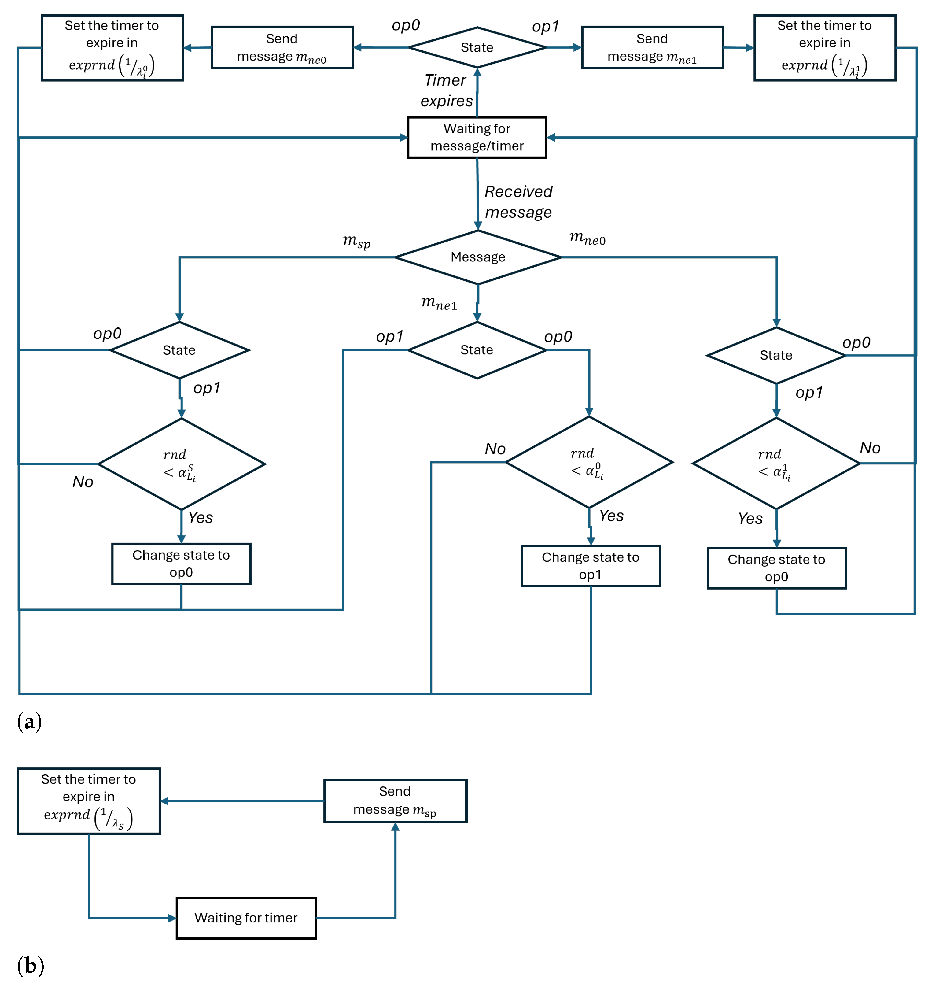
A block diagram illustrating the model dynamics protocol is shown in Figure 4. Specifically, Figure 4a shows the dynamics protocol of a generic listener belonging to class $L_i$ and fig:protocolb shows the dynamics protocol of the speaker.

When these agents are deployed over a space $\mathcal{V}$, the perception function ${\mathbf{u}}_m\left(\right)$ has to be defined between each couple of them for all the exchanged messages m. The values of $u_m(\mathbf{v},C,s,{\mathbf{v}}^{\prime },C^{\prime },s^{\prime })$ represent the probability that an agent of class C, in position $\mathbf{v}$, and in state s, perceives a message m generated by an agent of class $C^{\prime }$ in position ${\mathbf{v}}^{\prime }$ in state $s^{\prime }$. We assume the spread of the agents belonging to both the classes $L_0$ and $L_1$ over a $(n\times n)$ squared grid with one agent per grid cell; on the other hand, only one agent in the class $Sp$ is deployed. A position will be denoted by a couple $\mathbf{v}=(x,y)$, with $x,y\in \{0,\dots ,n-1\}$.

Whereas the messages emitted by the agent in class $Sp$ are perceived by all the others, we assume agents in the grid interact only with their immediate neighborhoods. Let us denote with ${\mathbf{v}}_s$ the position in the space where the only agent in class $Sp$ is located. The perception functions implementing the scenario we introduced above are:

$$\begin{array}{cc}\hfill & u_{m_{sp}}(\mathbf{v},L_i,op1,{\mathbf{v}}_s,Sp,op0)=1,\hfill \end{array}$$

(10)

$$\begin{array}{cc}\hfill & u_{m_{ne0}}(\mathbf{v},L_i,op1,{\mathbf{v}}^{\prime },L_j,op0)=\left\{\begin{array}{cc}1,\hfill & \forall \mathbf{v},{\mathbf{v}}^{\prime }\in \mathcal{V}:|x-x^{\prime }|+|y-y^{\prime }|=1\hfill \\ 0,\hfill & \mathrm{otherwise}\hfill \end{array}\right.,\hfill \end{array}$$

(11)

$$\begin{array}{cc}\hfill & u_{m_{ne0}}(\mathbf{v},L_i,op0,{\mathbf{v}}^{\prime },L_j,op1)=\left\{\begin{array}{cc}1,\hfill & \forall \mathbf{v},{\mathbf{v}}^{\prime }\in \mathcal{V}:|x-x^{\prime }|+|y-y^{\prime }|=1\hfill \\ 0,\hfill & \mathrm{otherwise}\hfill \end{array}\right.,\hfill \end{array}$$

(12)

$\forall i,j\in \{0,1\}$.

By solving a Markovian agent model, state probability vectors $\mathit{\pi }(t,\mathbf{v})$ of all deployed agents are derived. Their knowledge allows us to get information about the emerging opinion and how it takes form. In fact, we are able to derive whether an individual in position $\mathbf{v}$ tends to have either $Opinio{n}_0$ or $Opinio{n}_1$ at time t by evaluating state probabilities ${\mathit{\pi }}_0(t,\mathbf{v})$ and ${\mathit{\pi }}_1(t,\mathbf{v})$.

Although the scenario we implemented with the model above is inspired by an electoral rally, the latter is more general, and it is useful in many other real contexts.

5. Model Analysis and Numerical Results

In this section, we present and discuss results obtained by analyzing the model introduced in Section 4 under several conditions of parameter settings with the aim to show the potentiality of the proposed approach in exploring the related opinion dynamics behavior.

The performed experimentation aims to understand if the speaker is able to have the majority of consensus from the assembly assuming the crowd is heterogeneous. The space is a $(n\times n)$ grid and $N_0\left(t\right)$ agents, over $N=n\times n$, with opinion $op0$ are located in the space at time t; the remaining $N_1\left(t\right)=N-N_0\left(t\right)$ will have opinion $op1$. $N_0\left(t\right)$ and $N_1\left(t\right)$ are r.v. whose value at time $t=0$ depends on the spatial distribution of listeners. We experimented with two different scenarios: (1) the number of agents within both class $L_0$ and class $L_1$ are randomly scattered in the grid; (2) a similar initial fraction of agents has been set as in scenario, (1) but they have all been located in a rectangular area in the middle of the grid. The two scenarios are denoted Random and Rectangular, respectively. For instance, Figure 5 shows both Random and Rectangular initial distribution of individuals into a $20\times 20$ grid. Individuals with $Opinio{n}_0$ are depicted as a white box, whereas black boxes represent $Opinio{n}_1$ oriented individuals; $25\%$ of the population has $Opinio{n}_0$ in the scenarios depicted in Figure 5.

It is worth noting that even if the model here introduced has the aim to analyze the opinion dynamics of listeners during an election rally, its validity is much more general, and it can be used for several different applications. Due to the consideration above, we will not explicitly state the time unit used, leaving it general and denoting it simply with “u”. In the election rally application, it should be assumed to be “hours”.

Several parameters can be tuned in our proposed model: the induction rate of the agent in the $Sp$ class (${\lambda }_S$), and the induction rates of the agents in the $L_0$ and $L_1$ classes (${\lambda }_0^0$, ${\lambda }_0^1$, ${\lambda }_1^0$, ${\lambda }_1^1$); the perception probabilities that regulate the tendency to listen to the opinion of others (${\alpha }_0^S$, ${\alpha }_0^0$, ${\alpha }_0^1$, ${\alpha }_1^S$, ${\alpha }_1^0$, ${\alpha }_1^1$); and the relative number $r={\displaystyle \frac{N_1\left(0\right)}{N}}$ of agents in class $L_1$. We choose to keep the perception probabilities and the induction rates of $L_0$ and $L_1$ constant and to vary ${\lambda }_S$ and r. The parameter values used in our experimentation are summarized in

Table 3. Model parameter values; induction rate value unit is $1/u$.

n	N	${\mathit{\lambda }}_0^0$	${\mathit{\lambda }}_0^1$	${\mathit{\lambda }}_1^0$	${\mathit{\lambda }}_1^1$	${\mathit{\alpha }}_0^{\mathit{S}}$	${\mathit{\alpha }}_0^0$	${\mathit{\alpha }}_0^1$	${\mathit{\alpha }}_1^{\mathit{S}}$	${\mathit{\alpha }}_1^0$	${\mathit{\alpha }}_1^1$
20	400	$1.0$	$0.1$	$0.1$	$1.0$	$0.9$	$0.9$	$0.1$	$0.2$	$0.2$	$0.9$

.

The experimented scenario is made by 401 agents belonging to three classes as introduced in Section 3. The agent modeling the speaker is characterized by one state; all of the remaining 400 agents are made by two states, thus the model generates a system of 801 non-homogeneous ordinary differential equations as described in Section 3 and Section 5. We assumed a set of initial probability vectors as in Equation (7).

The generated ODE system has been numerically solved by exploiting explicit embedded Runge-Kutta solver evaluating 101 time points, from $0.0$ to $5.0$, with $0.05$ as step and tolerance equal to ${10}^{-6}$. The model has been implemented in C, with the support of MAGNET C library [22], which is a tool for the analysis of models based on the Markovian agent modeling paradigm (MAGNET is available at http://perf.unime.it/magnet/accessed on 22 May 2025). By exploiting MAGNET primitives, we implemented the description of agents’ structure (Equations (8) and (9)), their interactions (Equations (10)–(12)), and their spatial distribution. MAGNET implements the generation and solution of the ODE system.

Let $\mathrm{\Omega }\left(t\right)$ denote the number of agents with opinion $Opinio{n}_0$ at time t. It can be derived by counting the agents in state $op0$. It is easy to understand that, in a specific time instant $\overline{t}$, $\mathrm{\Omega }\left(\overline{t}\right)$ is a discrete random variable distributed according to a Poisson binomial distribution in a collection of $N=n\times n$ trials with success probabilities $\mathit{\pi }(\mathbf{v},\overline{t})$. Based on this latter remark, we evaluated the probability mass function of $\mathrm{\Omega }\left(\overline{t}\right)$, $f_{\mathrm{\Omega }\left(\overline{t}\right)}\left[k\right]$, and its expected value ${\mu }_{\mathrm{\Omega }}\left(\overline{t}\right)=E[\mathrm{\Omega }\left(\overline{t}\right)]$ as follows:

$$f_{\mathrm{\Omega }\left(\overline{t}\right)}\left[k\right]=\sum _{V\in {\mathcal{V}}_k}\prod _{\mathbf{v}\in V}{\pi }_0(\mathbf{v},\overline{t})\prod _{\mathbf{v}\in \overline{V}}(1-{\pi }_0(\mathbf{v},\overline{t})),$$

(13)

$${\mu }_{\mathrm{\Omega }}\left(\overline{t}\right)=\sum _{\mathbf{v}\in \mathcal{V}}{\pi }_0(\mathbf{v},\overline{t})$$

(14)

where ${\pi }_0(\mathbf{v},\overline{t})$ is the probability the agent in position $\mathbf{v}$ is in the state $op0$ at time $\overline{t}$, ${\mathcal{V}}_k$ is the set of all subsets of k positions in the grid, and $\overline{V}=\mathcal{V}-V$. Computation of $f_{\mathrm{\Omega }\left(\overline{t}\right)}\left[k\right]$ in Equation (13) is quite expensive but can be efficiently completed by exploiting the FFT like described in [26].

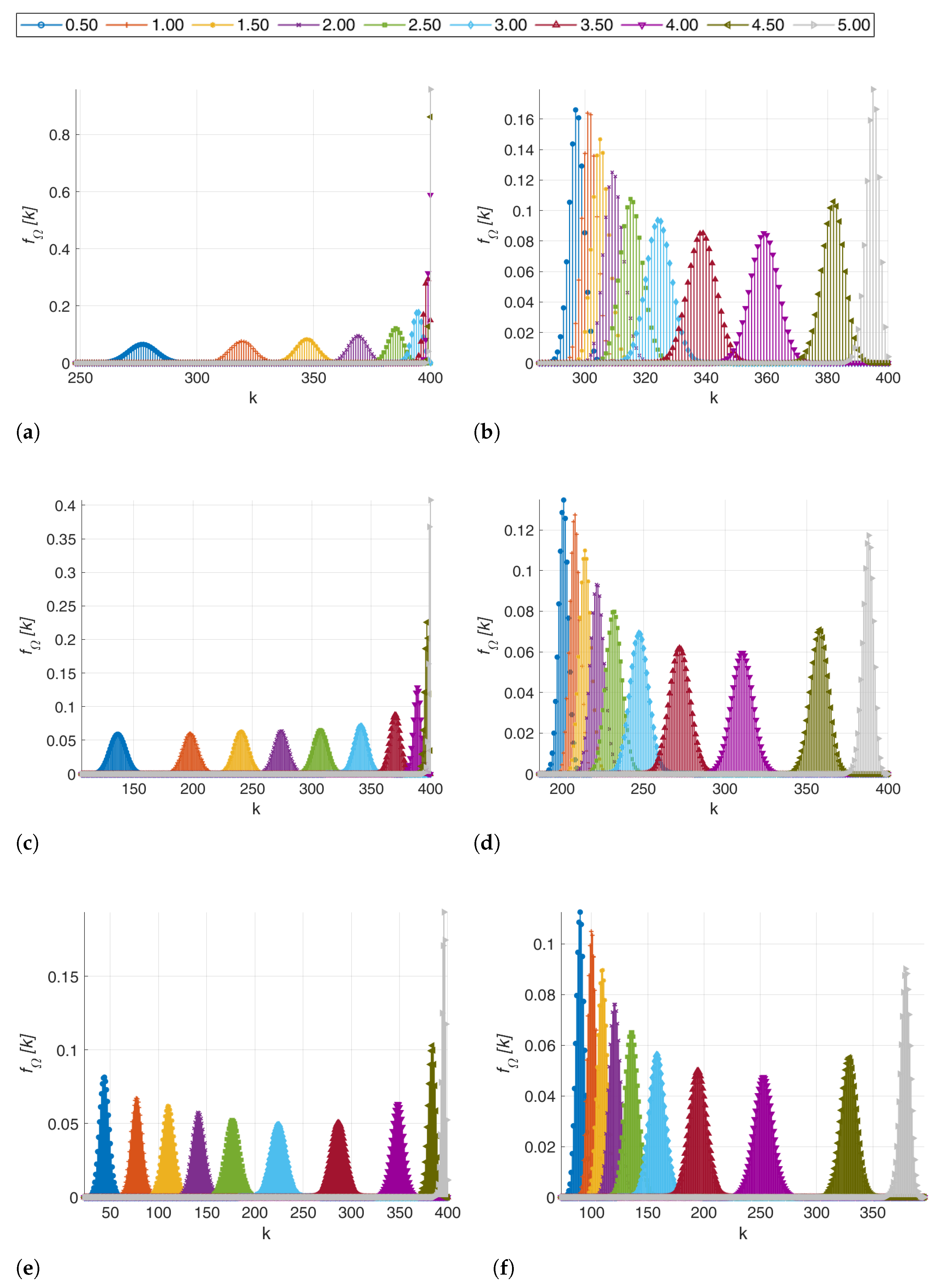
Figure 6 depicts $f_{\mathrm{\Omega }(\overline{t} = 2.5u)}\left[k\right]$ for both the two scenarios when the number of spread agents in class $L_1$ changes and the speaker induction rate is ${\lambda }_S=2.5u^{-1}$; we also put in evidence all the expected values in the ground 0 (red lines). Figure 6a,c,e are related to the Random scenario with $r=0.25,0.5,0.75$, respectively, whereas Figure 6b,d,f show results of the Rectangular one, assuming rectangular regions whose dimensions were $10\times 10$, $14\times 14$ and $17\times 18$; these latter are chosen in order to have the r parameter as similar as possible to the Random scenario ($r=0.25,0.49,0.77$) and make them comparable. The results show that Random scenarios produce more polarized final configurations of the speaker’s opinion, and also the mean value of agents with the same opinion of the speaker is higher even if the initial number of initial opponents is the same. 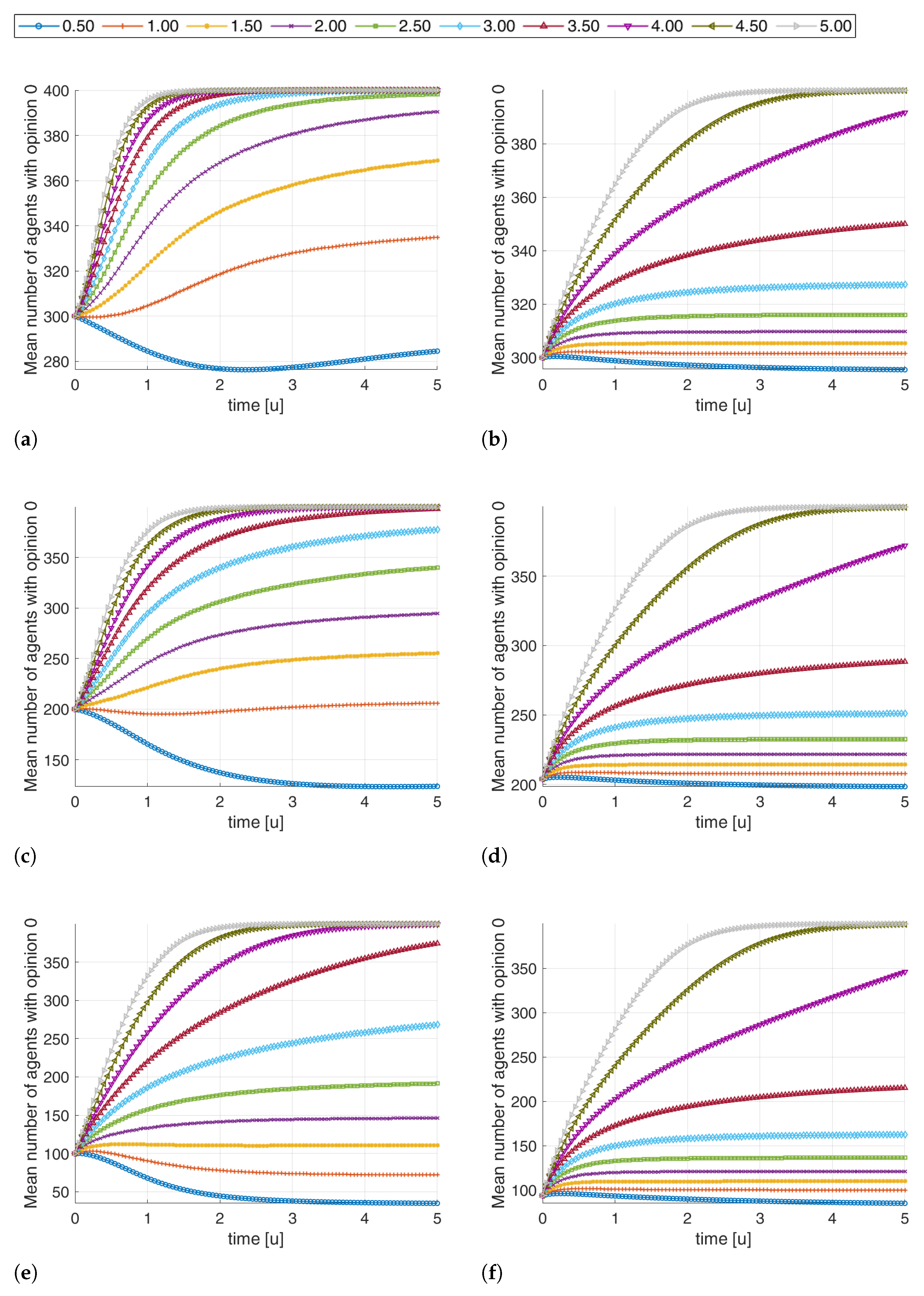Such a kind of dynamic is a general result; this is shown by the graphs of Figure 7, where the expected values of $\mathrm{\Omega }\left(t\right)$ are depicted for all the scenarios and with different speaker influence rates, as depicted in the legend; even if some degree of polarization is always reached, the Rectangular scenario is less prone to produce a diffusion of speaker opinion both in terms of the number of agents in class $L_1$ with a changed opinion and the time at which a given polarization level is reached because its dynamic is slower. This behavior is due to the fact that most of the agents in class $L_1$ (with an opinion different from the speaker) do not interact with agents in class $L_0$; thus, their opinion is reinforced from the neighbors (they support each other), and only a very good speaker, with ${\lambda }_S\ge 4.0u^{-1}$, can significantly produce a polarization toward its opinion.

One of the advantages of the model introduced in this work is the ability to derive transient measures, which are important when the application does not require knowledge of the steady state but of established time intervals, such as the case study of an electoral rally. In this sense, the set of distributions at a time instant of interest $\overline{t}$ can be analyzed to determine whether the required conditions are met. Figure 8 shows the set of $f_{\mathrm{\Omega }}\left[k\right]$ at $\overline{t}=0.25u$ parameterized with the speaker induction rates (written in the legend). We used different scale axes for making the drawing readable; otherwise, it is difficult to grasp the characteristics of the depicted distribution functions. We can see that when the speaker is not strong enough in convincing people with contrary opinions, just a few of them change their minds; it happens when ${\lambda }_S\le 1.5u^{-1}$ and $r=0.5$, when ${\lambda }_S\le 3.0u^{-1}$ and $r=0.75$ in the Random scenario, and when ${\lambda }_S\le 3.0u^{-1}$ and $r\simeq 0.5$ when ${\lambda }_S\le 4.0u^{-1}$ and $r\simeq 0.75$ in the Rectangular scenario. This is quite crucial information for planning the speaker’s speech within a given time instant $\overline{t}$.

Since the aim of a political rally is to convince as many people as possible in order to obtain a majority, we also evaluated the probability over time that at least half plus one of the people have reached the speaker’s opinion in the different scenarios. Figure 9 depicts the quantity $M_0\left(t\right)={\sum }_{k>\frac{N}{2}+1}{f}_{\mathrm{\Omega }}\left[k\right]$ that estimates the probability the majority of the agents has opinion $op0$ at different time points. From the graph, it is easy to see the final effect depends on both the speaker induction rate ${\lambda }_s$ (the parameter of the set of curves reported in the legend) and the time length. It is worth noting that spatial distribution also has its significance. Although in the scenario where $r=0.25$ there is a majority regardless of the speaker’s characteristics (Figure 9a,b), as expected, in the other situations it does not happen. In the Random scenario, it is necessary to have at least $2.5u$ of time for a reasonable certainty of reaching the majority when $r=0.5$, if the speaker has an influencing capacity equal to ${\lambda }_s=1.0u^{-1}$ (Figure 9c); while a speaker with ${\lambda }_S=3.0u^{-1}$ cannot reinforce the audience to keep the majority. In the Rectangular scenario, the situation improves when $r=0.5$, while it becomes worse than the Random scenario, where it is necessary to have an induction rate higher than $3.0$, and, in any case, it is necessary to have longer times, with the same speaker’s induction rate, to obtain high probabilities to reach the majority of the consensus. The speaker needs to devote more effort (Figure 9e,f) to convincing individuals when most of them are against the opinion of the speaker when the assembly starts (at $\overline{t}=0u$).

The last measure we evaluated is the time required for considering the transitory expired; that is important for evaluating when no new effects emerge from the agents. We defined the transitory expiration time $T_T$ as the first time after which the probability to be in state $op0$ remains under the threshold $h_T$ for all the agents spread over the grid. In order to compute the $T_T$ value, we introduce the resolution step ${\delta }_T$ and evaluate it as the quantity satisfying both of the two following statements:

$$\begin{array}{c}\exists T_T:\underset{\mathbf{v}\in V}{max}[{\pi }_0(\mathbf{v},T_T)-{\pi }_0(\mathbf{v},T_T-{\delta }_T)]\le h_T\\ \forall t<T_T\Rightarrow \underset{\mathbf{v}\in V}{max}[{\pi }_0(\mathbf{v},t)-{\pi }_0(\mathbf{v},t-{\delta }_T)]>h_T\end{array}$$

Figure 10 shows $T_T$ for the two scenarios when the speaker intensity changes, assuming $h_T=0.1$ and ${\delta }_T=0.05$. We can see that the Random scenario is very different from the Rectangular one; in the latter, the transitory expires similarly independently from the initial number of agents in a given class. Its maximum is around ${\lambda }_S=4.5$. At the opposite, the $T_T$ value in Random scenarios has very different behaviors depending on parameter values because the lack of symmetry makes each agent’s behavior different depending on the number of neighbors in a different class.

6. Conclusions and Future Works

In this paper, we propose the use of Markovian agents for agent-based opinion dynamics modeling. Markovian agents are particularly suitable for modeling asymmetric scenarios with different kinds of individuals, each with their own opinion, and complex scenarios.

The proposed Markovian agent modeling framework complements existing approaches by providing a versatile and analytically tractable tool for studying opinion dynamics in temporally and spatially structured settings.

We showed how the interactive Markovian agent modeling paradigm is able to capture interactions between individuals, also taking into account spatial distribution that affects their behavior.

Our model demonstrated the ability to simulate the dynamics of opinion formation and polarization in a crowd during an electoral rally, where a speaker attempts to influence listeners with diverse initial opinions. The results highlighted the importance of the speaker’s influence rate and the spatial distribution of listeners in determining the final consensus. Specifically, we observed that a higher speaker influence rate significantly increases the likelihood of achieving a majority consensus, particularly in scenarios where listeners are randomly distributed. Conversely, when listeners are clustered in a specific area, the speaker’s influence becomes less effective, and achieving consensus requires more time and a higher influence rate.

One of the key advantages of our model is its ability to derive transient measures, which are crucial for applications where the focus is on understanding the evolution of opinions over a specific time frame rather than reaching a steady state. This is particularly relevant in the context of political rallies, where the goal is to maximize the number of convinced listeners within a limited time period. Our analysis of the transient phase revealed that the spatial distribution of listeners plays a significant role in the speed and extent of opinion change, with random distributions leading to faster and more widespread consensus compared to clustered distributions.

Furthermore, the flexibility of our model allows incorporation of additional factors that could influence opinion dynamics, such as the presence of mass media or the introduction of multiple speakers with varying levels of influence. Future work could explore these extensions to provide a more comprehensive understanding of opinion formation in complex social networks.

Another area of interest is the extension of the model to include more complex network structures, such as scale-free or small-world networks, which better reflect real-world social interactions. This could help in understanding how the topology of social networks influences the spread of opinions and the formation of consensus.

Finally, empirical validation of the model using real-world data from political rallies, social media platforms, or other opinion-influencing events could enhance the model’s applicability and provide more accurate predictions of opinion dynamics in various contexts. We plan to experiment with the Markovian agent approach using real-world data in future work.