Structure Approximation-Based Preconditioning for Solving Tempered Fractional Diffusion Equations

Abstract

Tempered fractional diffusion equations constitute a critical class of partial differential equations with broad applications across multiple physical domains. In this paper, the Crank–Nicolson method and the tempered weighted and shifted Grünwald formula are used to discretize the tempered fractional diffusion equations. The discretized system has the structure of the sum of the identity matrix and a diagonal matrix multiplied by a symmetric positive definite (SPD) Toeplitz matrix. For the discretized system, we propose a structure approximation-based preconditioning method. The structure approximation lies in two aspects: the inverse approximation based on the row-by-row strategy and the SPD Toeplitz approximation by the $\tau$ matrix. The proposed preconditioning method can be efficiently implemented using the discrete sine transform (DST). In spectral analysis, it is found that the eigenvalues of the preconditioned coefficient matrix are clustered around 1, ensuring fast convergence of Krylov subspace methods with the new preconditioner. Numerical experiments demonstrate the effectiveness of the proposed preconditioner.

1. Introduction

This paper discusses the numerical solution of variable coefficient tempered fractional diffusion equations (tempered FDEs) with initial boundary value problems

$$\left\{\begin{array}{c}{\displaystyle \frac{\partial u\left(x,t\right)}{\partial t}}=d\left(x\right)\left({}_{\mathit{a}}{\mathit{D}}_{\mathit{x}}^{\mathit{\beta },\mathit{\lambda }}+{}_{\mathit{x}}{\mathit{D}}_{\mathit{b}}^{\mathit{\beta },\mathit{\lambda }}\right)u\left(x,t\right)+f\left(x,t\right),\hfill \\ u\left(a,t\right)=0,u\left(b,t\right)=0,t\in \left[0,T\right],\hfill \\ u\left(x,0\right)=u_0\left(x\right),x\in \left[a,b\right],\hfill \end{array}\right.$$

(1)

where $f(x,t)$ is the source term, $d\left(x\right)\ge 0$ is the diffusion coefficient function, and $\lambda$ is a non-negative parameter. ${}_{\mathit{a}}{\mathit{D}}_{\mathit{x}}^{\mathit{\beta },\mathit{\lambda }}$ and ${}_{\mathit{x}}{\mathit{D}}_{\mathit{b}}^{\mathit{\beta },\mathit{\lambda }}$ denote the left and right Riemann–Liouville tempered fractional derivatives of the function $u(x,t)$ with order $\beta \left(1<\beta <2\right)$, respectively. They are defined by (see Baeumer and Meerschaert [1])

$${}_{\mathit{a}}{\mathit{D}}_{\mathit{x}}^{\mathit{\beta },\mathit{\lambda }}u\left(x\right)={}_a{D}_x^{\beta ,\lambda }u\left(x\right)-\beta {\lambda }^{\beta -1}{\partial }_{x}u\left(x\right)-{\lambda }^{\beta }u\left(x\right)$$

and

$${}_{\mathit{x}}{\mathit{D}}_{\mathit{b}}^{\mathit{\beta },\mathit{\lambda }}u\left(x\right)={}_x{D}_b^{\beta ,\lambda }u\left(x\right)+\beta {\lambda }^{\beta -1}{\partial }_{x}u\left(x\right)-{\lambda }^{\beta }u\left(x\right)$$

where

$${}_a{D}_x^{\beta ,\lambda }u\left(x\right)={\mathrm{e}}^{-\lambda x}{}_a{D}_x^{\beta }\left({\mathrm{e}}^{\lambda x}u\left(x\right)\right)={\displaystyle \frac{{\mathrm{e}}^{-\lambda x}}{\Gamma \left(2-\beta \right)}}{\displaystyle \frac{{\partial }^2}{\partial x^2}}{\int }_a^x{\displaystyle \frac{{\mathrm{e}}^{\lambda s}u\left(s\right)}{{\left(x-s\right)}^{\beta -1}}}ds$$

and

$${}_x{D}_b^{\beta ,\lambda }u\left(x\right)={\mathrm{e}}^{\lambda x}{}_x{D}_b^{\beta }\left({\mathrm{e}}^{-\lambda x}u\left(x\right)\right)={\displaystyle \frac{{\mathrm{e}}^{\lambda x}}{\Gamma \left(2-\beta \right)}}{\displaystyle \frac{{\partial }^2}{\partial x^2}}{\int }_x^b{\displaystyle \frac{{\mathrm{e}}^{-\lambda s}u\left(s\right)}{{\left(s-x\right)}^{\beta -1}}}ds.$$

Tempered FDEs are a crucial class of equations widely applied in fields such as biology, geophysics, and finance [2,3,4]. These equations are characterized by incorporating tempered fractional derivatives, modifying standard fractional diffusion equations by introducing an exponential tempering factor. This modification allows tempered FDEs to better simulate processes with finite propagation speed, accurately describing actual physical phenomena. However, analytical solutions to tempered FDEs and FDEs are generally difficult to obtain, leading to extensive research on the numerical solutions of FDEs in recent years [5,6,7,8,9,10,11].

For tempered fractional derivatives, stability of the resulting finite difference schemes can only be ensured if the spatial step size is sufficiently small when using standard fractional derivative approximations directly [12]. A novel shifted approximation method for tempered fractional derivatives was proposed in [13], successfully developing an unconditionally stable numerical scheme for one-dimensional (1D) tempered fractional diffusion equations with constant coefficients. Additionally, a Crank–Nicolson scheme was proposed [14] for solving initial boundary value problems of a class of variable coefficient tempered fractional diffusion equations, providing the discretization method used in this paper. The inherent non-locality of tempered fractional operators manifests in the algebraic structure of discretized systems, producing coefficient matrices with dense or fully populated configurations. The system’s coefficient matrix assumes the configuration $I+DT$, with I denoting the identity matrix, D a diagonal matrix, and T an SPD Toeplitz matrix.

Traditional direct solution methods, such as Gaussian elimination, require large computational cost and storage space. The Krylov subspace methods are typically used to solve these kinds of linear system. Meanwhile, effective preconditioning strategies can significantly accelerate the convergence rate of the Krylov subspace methods [15,16,17,18]. For 1D and 2D tempered FDEs, Lei, Fan and Chen [19] proposed a fast-iterative method and a fast-direct method. And they used the circulant preconditioner to accelerate the iteration process. In [20], a robust preconditioner was developed for the discretized scheme of nonlinear tempered FDEs. In [21], a circulant and skew-circulant splitting iteration method was used to solve the discretized system of tempered FDEs. The induced preconditioning form was also investigated. Nevertheless, emerging methodologies demonstrate superior efficacy compared to conventional preconditioning approaches. For 1D tempered FDEs, Tang and Huang [22] approximated the SPD Toeplitz matrix by the $\tau$ matrix [15] and proposed a scaled diagonal and Toeplitz approximate splitting (SDTAS) preconditioning method. The equations examined in this study address a notably underexplored class of tempered FDEs in the contemporary literature, characterized by discretization schemes that yield coefficient matrices incorporating SPD Toeplitz structures. This distinctive matrix configuration, possessing both theoretically significant properties and practical computational advantages, constitutes the principal focus of our numerical investigation. Also, some of the latest numerical solution methods for FDEs are described in [23,24]. In addition, it is noticed that a row-by-row inverse approximation strategy has been proposed [25] and applied [26,27,28]. Inspired by this strategy, we will try to construct an efficient preconditioner for the linear system arising from the numerical solution of tempered FDEs with variable coefficients.

In this paper, we use the second-order finite difference scheme to discretize the tempered FDEs. Specifically, we employ the Crank–Nicolson method for time discretization and the tempered weighted and shifted Grünwald formula for spatial discretization. We observe that the coefficient matrix of the resulting linear system is of the form $I+DT$. We approximate the SPD Toeplitz matrix T by the $\tau$ matrix and construct a novel approximate inverse preconditioner inspired by the row-by-row approximation strategy. The preconditioner can be efficiently computed using discrete sine transforms, with each step of the preconditioned Krylov subspace method having a computational complexity of $O(NlogN)$. Spectral analysis establishes eigenvalue clustering near unity for the preconditioned system, which theoretically guarantees the superlinear convergence rate of Krylov subspace iterations—a property rigorously verified through our mathematical proofs. Numerical experiments are carried out to assess the performance of the developed preconditioner.

The remainder of this paper is organized as follows. Section 2 presents the derivation of the discretized system for tempered FDEs. Section 3 details the formulation of an approximate inverse preconditioner. Section 4 performs spectral analysis of the preconditioned matrices. Section 5 validates the computational efficiency of the proposed preconditioner through numerical experiments. Concluding remarks summarizing the key findings are provided in Section 6.

2. Discretization of Tempered FDEs

Let N and M be positive integers, representing the number of spatial and temporal partitions, respectively. We define the spatial step size $h={\displaystyle \frac{a}{N+1}}$ and the time step size $\Delta t={\displaystyle \frac{T}{M}}$. The spatial and temporal grids are given by $x_i=ih$ for $i=0,1,\dots ,N+1$ and $t_j=j\Delta t$ for $j=0,1,\dots ,M$.

We review that the tempered fractional derivatives in (1) can be approximated using the tempered weighted and shifted Grünwald formula (tempered WSGD) [14]

$${}_{a}D_x^{\beta ,\lambda }u\left(x_i,t_j\right)-{\lambda }^{\beta }u\left(x_i,t_j\right)={\displaystyle \frac{1}{h^{\beta }}}\sum _{k=0}^{i+1}{g}_k^{\left(\beta \right)}u\left(x_{i-k+1},t_j\right)-{\displaystyle \frac{1}{h^{\beta }}}{\rho }_{\beta }u\left(x_i,t_j\right)+O\left(h^2\right),$$

and

$${}_{x}D_b^{\beta ,\lambda }u\left(x_i,t_j\right)-{\lambda }^{\beta }u\left(x_i,t_j\right)={\displaystyle \frac{1}{h^{\beta }}}\sum _{k=0}^{N-i+2}{g}_k^{\left(\beta \right)}u\left(x_{i+k-1},t_j\right)-{\displaystyle \frac{1}{h^{\beta }}}{\rho }_{\beta }u\left(x_i,t_j\right)+O\left(h^2\right),$$

where ${\rho }_{\beta }=\left({\gamma }_1{e}^{h\lambda }+{\gamma }_2+{\gamma }_3{e}^{-h\lambda }\right){\left(1-e^{-h\lambda }\right)}^{\beta }$; the weights $g_k^{\left(\beta \right)}$ are given by

$$g_k^{\left(\beta \right)}=\left\{\begin{array}{cc}{\gamma }_1{w}_0^{\left(\beta \right)}{e}^{h\lambda },\hfill & k=0,\hfill \\ {\gamma }_1{w}_1^{\left(\beta \right)}+{\gamma }_2{w}_0^{\left(\beta \right)},\hfill & k=1,\hfill \\ \left({\gamma }_1{w}_k^{\left(\beta \right)}+{\gamma }_2{w}_{k-1}^{\left(\beta \right)}+{\gamma }_3{w}_{k-2}^{\left(\beta \right)}\right)e^{-\left(k-1\right)h\lambda },\hfill & k\ge 2,\hfill \end{array}\right.$$

(2)

where $w_0^{\left(\beta \right)}=1,w_k^{\left(\beta \right)}=\left(1-{\displaystyle \frac{1+\beta }{k}}\right)w_{k-1}^{\left(\beta \right)},\mathrm{for}k\ge 1$, and ${\gamma }_1,{\gamma }_2,{\gamma }_3$ satisfy the linear system

$$\left\{\begin{array}{c}{\gamma }_1+{\gamma }_2+{\gamma }_3=1,\hfill \\ {\gamma }_1-{\gamma }_3=\beta /2.\hfill \end{array}\right.$$

(3)

Let $u_i^j\approx u\left(x_i,t_j\right),f_i^{j+{\displaystyle \frac{1}{2}}}=f\left(x_i,t_{j+{\displaystyle \frac{1}{2}}}\right),t_{j+{\displaystyle \frac{1}{2}}}={\displaystyle \frac{1}{2}}\left(t_j+t_{j+1}\right)$ and $u_i^{j+{\displaystyle \frac{1}{2}}}={\displaystyle \frac{1}{2}}\left(u_i^j+u_i^{j+1}\right)$ for $i=1,\dots ,N,j=0,1,\dots ,M$. At the mesh point $\left(x_i,t_{j+{\displaystyle \frac{1}{2}}}\right)$, we consider the Crank–Nicolson technique for time discretization and the tempered WSGD approximation for the tempered fractional derivatives to discretize the tempered FDEs in (1). Under the truncation-error-free assumption [23,24], the second-order finite difference scheme is formulated as follows:

$$\begin{array}{cc}\hfill {\displaystyle \frac{u_i^{j+1}-u_i^j}{\Delta t}}=& {\displaystyle \frac{d_i}{2}}\left({\displaystyle \frac{1}{h^{\beta }}}\sum _{k=0}^{i+1}{g}_k^{\left(\beta \right)}{u}_{i-k+1}^{j+1}-{\displaystyle \frac{1}{h^{\beta }}}{\rho }_{\beta }{u}_i^{j+1}+{\displaystyle \frac{1}{h^{\beta }}}\sum _{k=0}^{N-i+2}{g}_k^{\left(\beta \right)}{u}_{i+k-1}^{j+1}-{\displaystyle \frac{1}{h^{\beta }}}{\rho }_{\beta }{u}_i^{j+1}\right)\hfill \\ \hfill & +{\displaystyle \frac{d_i}{2}}\left({\displaystyle \frac{1}{h^{\beta }}}\sum _{k=0}^{i+1}{g}_k^{\left(\beta \right)}{u}_{i-k+1}^j-{\displaystyle \frac{1}{h^{\beta }}}{\rho }_{\beta }{u}_i^j+{\displaystyle \frac{1}{h^{\beta }}}\sum _{k=0}^{N-i+2}{g}_k^{\left(\beta \right)}{u}_{i+k-1}^j-{\displaystyle \frac{1}{h^{\beta }}}{\rho }_{\beta }{u}_i^j\right)\hfill \\ \hfill & +f_i^{j+{\displaystyle \frac{1}{2}}}.\hfill \end{array}$$

(4)

We define the diagonal matrix as

$$D=\mathrm{diag}\left(d_1,d_2,\dots ,d_N\right)$$

and the vectors as

$$u^j={\left[u_1^j,u_2^j,\dots ,u_N^j\right]}^T,f^{j+{\displaystyle \frac{1}{2}}}={\left[f_1^{j+{\displaystyle \frac{1}{2}}},f_2^{j+{\displaystyle \frac{1}{2}}},\dots ,f_N^{j+{\displaystyle \frac{1}{2}}}\right]}^T.$$

For $j=0,1,\dots ,M$ and a given $u^0$, the differential scheme (4) admits a matrix representation expressed as

$$\left(I+DG\right)u^{j+1}=\left(I-DG\right)u^j+\Delta t{f}^{j+{\displaystyle \frac{1}{2}}},$$

(5)

where I is the identity matrix, and G is an SPD Toeplitz matrix, defined as $G=G_{\beta }+G_{\beta }^T$, where $G_{\beta }^T$ represents the transpose of $G_{\beta }$. $G_{\beta }$ can be represented as

$$G_{\beta }=-{\displaystyle \frac{\Delta t}{2h^{\beta }}}\left(\begin{array}{cccccc}{g}_1^{\left(\beta \right)}-{\rho }_{\beta }& g_0^{\left(\beta \right)}& 0& \dots & 0& 0\\ g_2^{\left(\beta \right)}& g_1^{\left(\beta \right)}-{\rho }_{\beta }& g_0^{\left(\beta \right)}& 0& \dots & 0\\ ⋮& \ddots & \ddots & \ddots & & ⋮\\ g_{N-1}^{\left(\beta \right)}& \ddots & \ddots & \ddots & & g_0^{\left(\beta \right)}\\ g_N^{\left(\beta \right)}& g_{N-1}^{\left(\beta \right)}& \dots & \dots & g_2^{\left(\beta \right)}& g_1^{\left(\beta \right)}-{\rho }_{\beta }\end{array}\right).$$

Consequently, the coefficient matrix A associated with the tempered FDEs (4) is structured as a superposition of the identity matrix and an SPD Toeplitz matrix premultiplying a diagonal matrix, analytically expressed as

$$A=I+DG.$$

(6)

Since the system (3) is underdetermined, the following Lemma 1 [14] establishes additional constraints on parameters ${\gamma }_1,{\gamma }_2,{\gamma }_3$ to ensure that the finite difference scheme (4) remains unconditionally stable while attaining second-order accuracy in both spatial and temporal domains.

Lemma 1.

Let S be the solution set of the linear system (3), if $1<\beta <2$, $\lambda \ge 0,\left({\gamma }_1,{\gamma }_2,{\gamma }_3\right)\in \mathcal{S},and$

$$\begin{array}{c}1.max\left\{{\displaystyle \frac{2\left({\beta }^2+3\beta -4\right)}{{\beta }^2+3\beta +2}},{\displaystyle \frac{{\beta }^2+3\beta }{{\beta }^2+3\beta +4}}\right\}<{\gamma }_1<{\displaystyle \frac{3\left({\beta }^2+3\beta -2\right)}{2\left({\beta }^2+3\beta +2\right)}};or\hfill \\ 2.{\displaystyle \frac{\left(\beta -4\right)\left({\beta }^2+3\beta +2\right)+24}{2\left({\beta }^2+3\beta +2\right)}}<{\gamma }_2<min\left\{{\displaystyle \frac{\left(\beta -2\right)\left({\beta }^2+3\beta +4\right)+16}{2\left({\beta }^2+3\beta +4\right)}},{\displaystyle \frac{\left(\beta -6\right)\left({\beta }^2+3\beta +2\right)+48}{2\left({\beta }^2+3\beta +2\right)}}\right\};or\hfill \\ 3.max\left\{{\displaystyle \frac{\left(2-\beta \right)\left({\beta }^2+\beta -8\right)}{{\beta }^2+3\beta +2}},{\displaystyle \frac{\left(1-\beta \right)\left({\beta }^2+2\beta \right)}{2\left({\beta }^2+3\beta +4\right)}}\right\}<{\gamma }_3<{\displaystyle \frac{\left(2-\beta \right)\left({\beta }^2+2\beta -3\right)}{2\left({\beta }^2+3\beta +2\right)}}\hfill \end{array}$$

we have

$$g_1^{\left(\beta \right)}<0,g_2^{\left(\beta \right)}+g_0^{\left(\beta \right)}>0,g_k^{\left(\beta \right)}>0,\forall k\ge 3,\sum _{k=0}^{\infty }{g}_k^{\left(\beta \right)}={\rho }_{\beta }\ge 0.$$

(7)

3. Structure Approximation-Based Preconditioning

In this section, we first construct an inverse approximation for the coefficient matrix based on its structure and the row-by-row strategy. In addition, we approximated the involved SPD Toeplitz matrix by the corresponding $\tau$ matrix, thereby introducing a structure approximation-based preconditioner to address the targeted linear system (5).

The row-by-row approximation strategy [25] takes advantage of the fact that $e_i^{T}A=e_i^T{K}_i$. Here we take the approximation as $e_i^T{A}^{-1}\approx e_i^T{K}_i^{-1}$, where $e_i$ represents the i-th column of the identity matrix, $K_i=I+d_{i}G,i=1,2,\dots ,N$. Based on this, we obtain the approximate inverse preconditioner $P_1$

$$P_1^{-1}=\sum _{i=1}^N{e}_i{e}_i^T{K}_i^{-1}.$$

Recognizing that G exhibits an SPD Toeplitz structure, we employ the $\tau$-based matrix to derive an efficient approximation of G [15]. For convenience, the first column of the G matrix can be expressed as $-{\displaystyle \frac{\Delta t}{2h^{\beta }}}{\left[2\left(g_1^{\left(\beta \right)}-{\rho }_{\alpha }\right),g_0^{\left(\beta \right)}+g_2^{\left(\beta \right)},g_3^{\left(\beta \right)},\dots ,g_N^{\left(\beta \right)}\right]}^T$. According to [15], we can compute the $\tau$ matrix approximation using Hankel correction

$$\tau \left(G\right)=G-HC\left(G\right),$$

(8)

where $HC\left(G\right)$ is a symmetric Hankel matrix, and its anti-diagonal elements can be computed from the corresponding elements in the following first column and last column:

$$-{\displaystyle \frac{\Delta t}{2h^{\beta }}}{\left(g_3^{\left(\beta \right)},g_4^{\left(\beta \right)},\dots ,g_N^{\left(\beta \right)},0,0\right)}^T,-{\displaystyle \frac{\Delta t}{2h^{\beta }}}{\left(0,0,g_N^{\left(\beta \right)},\dots ,g_4^{\left(\beta \right)},g_3^{\left(\beta \right)}\right)}^T.$$

(9)

It is well-known that $\tau \left(G\right)$ defined in (8) admits diagonalization via the discrete sine transform:

$$\tau \left(G\right)=S\Lambda S,S=\left(\sqrt{{\displaystyle \frac{2}{N+1}}}·sin{\displaystyle \frac{\pi ij}{N+1}}\right),i,j=1,2,\dots ,N,$$

(10)

where $\Lambda =\mathrm{diag}\left({\lambda }_1,{\lambda }_2,\dots ,{\lambda }_N\right)$, and S is the discrete sine transform matrix.

Clearly, $G_j=I+d_j\tau \left(G\right)$ remains a $\tau$ matrix. Using the $\tau$ matrix $G_j$ to approximate the SPD Toeplitz matrix $K_j$, we obtain the $\tau$ matrix-based approximate preconditioner

$$P_2^{-1}=\sum _{i=1}^N{e}_i{e}_i^T{G}_i^{-1}.$$

(11)

With the preconditioner $P_2^{-1}$, we need to compute $O\left(N\right)$ discrete sine transforms for each iteration, which is still computationally intensive. As carried out in [25], we consider using interpolation methods to reduce computational complexity.

Define ${\left\{x_i\right\}}_{i=1}^N$ as the set of all discrete points in the interval $[a,b]$, and the function $q_k\left(x\right)={\displaystyle \frac{1}{1+{\lambda }_{k}d\left(x\right)}}$, where ${\lambda }_k\in sp\left(\tau \left(G\right)\right)=\{{\lambda }_1,{\lambda }_2,\dots ,{\lambda }_N\},k=1,2,\dots ,N$. Select $l\left(l\ll N\right)$ interpolation points ${\left\{\left({\tilde{x}}_j,q_k\left({\tilde{x}}_j\right)\right)\right\}}_{j=1}^l$ in $\left(x_i,q_k\left(x_i\right)\right){\}}_{i=1}^N$, and then piecewise linear interpolation is applied to construct the interpolating function

$$\begin{array}{cc}\hfill p_k\left(x\right)& ={\varphi }_1\left(x\right)q_k\left({\tilde{x}}_1\right)+{\varphi }_2\left(x\right)q_k\left({\tilde{x}}_2\right)+\cdots +{\varphi }_l\left(x\right)q_k\left({\tilde{x}}_l\right)\hfill \\ \hfill & =\sum _{s=1}^l{\varphi }_s\left(x\right)q_k\left({\tilde{x}}_s\right).\hfill \end{array}$$

(12)

By leveraging Equation (10), each $G_j$ is diagonalized into the form $G_j=S{\Lambda }_{j}S$ for $j=1,2,\dots ,N$ where S denotes the discrete sine transform matrix, and ${\Lambda }_j$ represents a diagonal matrix containing the eigenvalues of $G_j$. Then, applying interpolation (12) to approximate $G_j^{-1}$, we have

$$G_j^{-1}\approx S\left(\sum _{s=1}^l{\varphi }_s\left(x_j\right){\Lambda }_s^{-1}\right)S.$$

(13)

Replacing $G_j^{-1}$ in (11) with approximation values (13), we propose the approximate inverse preconditioner as

$$\begin{array}{cc}\hfill P_3^{-1}& =\sum _{i=1}^N{e}_i{e}_i^{T}S\left(\sum _{s=1}^l{\varphi }_s\left(x_i\right){\Lambda }_s^{-1}\right)S\hfill \\ \hfill & =\sum _{s=1}^l\left(\sum _{i=1}^N{e}_i{e}_i^T{\varphi }_s\left(x_i\right)\right)S\left({\Lambda }_s^{-1}\right)S\hfill \\ \hfill & =\sum _{s=1}^l{\Phi }_{s}S{\Lambda }_s^{-1}S,\hfill \end{array}$$

(14)

where ${\Phi }_s=diag\left({\phi }_s\left(x_1\right),{\phi }_s\left(x_2\right),\dots ,{\phi }_s\left(x_N\right)\right)$, ${\Lambda }_s^{-1}$= diag$\left(q_1\left({\tilde{x}}_s\right),q_2\left({\tilde{x}}_s\right),\dots ,q_N\left({\tilde{x}}_s\right)\right)$, $s=1,2,\dots ,l$ are diagonal matrices. For a suitable number of interpolation points l, the computation of the preconditioner (14) requires $O\left(lNlogN\right)$ operations. We denote $P_3^{-1}$ as $P_{TAI}^{-1}\left(l\right)$, where l represents the number of interpolation points, and have summarized the Algorithm 1 in the table below.

Algorithm 1 Solving system (5) by the PGMRES method with preconditioner $P_{TAI}^{-1}\left(l\right)$.

Input: Matrix $A=I+DG$ defined in (6) and the interpolation point l. Output: The solution $u=[u_1,u_2,\dots ,u_m]$. 1: Calculate the eigenvalues of G by FFT and calculate the eigenvalues of $\tau \left(G\right)$ by DST; 2: Construct the preconditioner $P_{TAI}^{-1}\left(l\right)$ by diagonalizing $\tau \left(G\right)$ using Formula (14); 3: Set the initial vector $u^0$; 4: For $k=1,2,\dots ,m$ do 5: Use the right-hand term of Formula (5) to calculate $b_k$ by FFT. 6: Calculate $P_{TAI}^{-1}\left(l\right)v$ by DST and calculate Av by FFT. 7: Obtain $u_k$ by performing MATLAB’s gmres. 8: end for

4. Spectral Analysis

In this section, we discuss the spectral properties of the preconditioned matrix $P_3^{-1}A$. First, we review some off-diagonal decay property reasoning.

Lemma 2

([25]). Let $\beta \in (1,2)$ and $A=\left(a_{i,j}\right)\in {\mathcal{L}}_{\beta +1}$ be a matrix, which satisfies

$$|a_{i,j}|\le {\displaystyle \frac{c}{{(1+|i-j\left|\right)}^{\beta +1}}}$$

for $\beta >0$, and some constant $c>0$. Then ∃ a constant ϖ s.t. ${\parallel L\parallel }_{\infty }\le \varpi$.

Lemma 3

([25]). Let A and $P_1$ be as defined in Section 3, $d\left(x\right)\in C^1[x_L,x_R]$. For any given $\epsilon >0$, there exists a constant $c_1$ and an integer $N_1$, such that for $l\ge N_1$,

$$\parallel P_1^{-1}-A^{-1}{\parallel }_{\infty }\le c_1\underset{1\le i\le N}{max}\Delta (x_i,l)+\epsilon ,$$

where

$$\Delta (x_i,l)=\underset{i-l\le k\le i+l}{max}|x_k-x_i|=(l-1)h.$$

Next, we discuss the spectral properties of $P_3^{-1}A$ by analyzing the approximation $P_3^{-1}-A^{-1}$. Due to

$$P_3^{-1}-A^{-1}=P_3^{-1}-P_2^{-1}+P_2^{-1}-P_1^{-1}+P_1^{-1}-A^{-1},$$

we will respectively analyze the properties of $P_3^{-1}-P_2^{-1},P_2^{-1}-P_1^{-1}$ and $P_1^{-1}-A^{-1}$. And the approximation property of $P_1$ and A is given in Lemma 3 above. Then, we give the results of the approximation property of $P_2^{-1}$ and $P_1^{-1}$.

Theorem 1.

Let $P_1$ and $P_2$ be defined as in Section 3. The approximation $P_2^{-1}$ to $P_1^{-1}$ satisfies

$$P_2^{-1}-P_1^{-1}=E_2+F_2,$$

where $E_2$ and $F_2$ are matrices of small norm and low rank, respectively, i.e., $\parallel E_2\parallel <c_2·ϵ$ and $\mathit{rank}\left(F_2\right)\le 4\varsigma$ for some positive constant $c_2$, ϵ and ς.

Proof. 

We can write $P_2^{-1}-P_1^{-1}$ as

$$\begin{array}{cc}\hfill P_2^{-1}-P_1^{-1}& =\sum _{i=1}^N{e}_i{e}_i^T\left(G_i^{-1}-K_i^{-1}\right)\hfill \\ & =\sum _{i=1}^N{e}_i{e}_i^T{K}_i^{-1}\left(K_i-G_i\right)G_i^{-1}\hfill \\ & =\sum _{i=1}^N{d_{i}e}_i{e}_i^T{K}_i^{-1}\left(G-\tau \left(G\right)\right)G_i^{-1},\hfill \end{array}$$

where $\parallel G_i^{-1}{\parallel }_{\infty }<{\eta }^{-1}$; for detailed proof, refer to Lemma 4.7 in [25].

As shown in [15], the matrix difference $G-\tau \left(G\right)$ admits a decomposition $E_1+F_1$, where $E_1$ coincides with $G-\tau \left(G\right)$ within the upper-left and lower-right $(N-1)\times (N-1)$ submatrices and vanishes elsewhere, while satisfying $rank\left(E_1\right)\le 2(N-1)$. Further, if we let $\epsilon >0$ be fixed, then we have $\parallel F_1{\parallel }_2<\epsilon .$

Given that $K_i^{-1}$ exhibits off-diagonal decay, it admits a splitting ${\tilde{K}}_i+{\widehat{K}}_i$, where

$${\tilde{K}}_i=\left[\begin{array}{cccccc}\ast & \cdots & \ast & 0& \cdots & 0\\ ⋮& \ddots & & \ddots & \ddots & ⋮\\ & & \ddots & & \ddots & 0\\ 0& \ddots & & \ddots & & \ast \\ ⋮& \ddots & \ddots & & \ddots & ⋮\\ 0& \cdots & 0& \ast & \cdots & \ast \end{array}\right]\mathrm{and}{\widehat{K}}_i=\left[\begin{array}{cccccc}0& \cdots & 0& \ast & \cdots & \ast \\ ⋮& \ddots & & \ddots & \ddots & ⋮\\ 0& & \ddots & & \ddots & \ast \\ & \ddots & & \ddots & & 0\\ ⋮& \ddots & \ddots & & \ddots & ⋮\\ & \cdots & \ast & 0& \cdots & 0\end{array}\right],$$

where ‘*’ denotes the nonzero entries.

Considering

$$\begin{array}{cc}\hfill K_i^{-1}(G-\tau \left(G\right))G_i^{-1}& =K_i^{-1}(E_1+F_1)G_i^{-1}\hfill \\ \hfill & =K_i^{-1}{E}_1{G}_i^{-1}+K_i^{-1}{F}_1{G}_i^{-1}\hfill \\ \hfill & =K_i^{-1}{E}_1{G}_i^{-1}+({\tilde{K}}_i+{\widehat{K}}_i)F_1{G}_i^{-1}\hfill \\ \hfill & =(K_i^{-1}{E}_1+{\widehat{K}}_i{F}_1)G_i^{-1}+{\tilde{K}}_i{F}_1{G}_i^{-1},\hfill \end{array}$$

we derive

$$\begin{array}{cc}\hfill \parallel (K_i^{-1}{E}_1+{\widehat{K}}_i{F}_1)G_i^{-1}{\parallel }_{\infty }& \le (\parallel K_i^{-1}{\parallel }_{\infty }·\parallel E_1{\parallel }_{\infty }+\parallel {\widehat{K}}_i{\parallel }_{\infty }·\parallel F_1{\parallel }_{\infty })·\parallel G_i^{-1}{\parallel }_{\infty }\hfill \\ \hfill & \le \epsilon (\parallel K_i^{-1}{\parallel }_{\infty }+\parallel F_1{\parallel }_{\infty })·\parallel G_i^{-1}{\parallel }_{\infty }\hfill \end{array}$$

and

$$\begin{array}{cc}\hfill \Vert \sum _{i=1}^N{e}_i{e}_i^T(K_i^{-1}{E}_1+{\widehat{K}}_i{F}_1)G_i^{-1}{\Vert }_{\infty }& =\underset{1\le i\le N}{max}{\parallel e_i^T(K_i^{-1}{E}_1+{\widehat{K}}_i{F}_1)G_i^{-1}\parallel }_1\hfill \\ \hfill & =\underset{1\le i\le N}{max}{\parallel (K_i^{-1}{E}_1+{\widehat{K}}_i{F}_1)G_i^{-1}\parallel }_{\infty }\hfill \\ \hfill & \le \epsilon ·\underset{1\le i\le N}{max}(\parallel K_i^{-1}{\parallel }_{\infty }+\parallel F_1{\parallel }_{\infty })·\parallel G_i^{-1}{\parallel }_{\infty }.\hfill \end{array}$$

Since $\parallel K_i^{-1}{\parallel }_{\infty }$ and $\parallel F_1{\parallel }_{\infty }$ are limited due to Lemma 2, it follows that $\parallel G_i^{-1}{\parallel }_{\infty }$ is also bounded. In other words, there is a constant $c_2>0$ such that

$${∥\sum _{i=1}^N{e}_i{e}_i^T(K_i^{-1}{E}_1+{\widehat{K}}_i{F}_1)G_i^{-1}∥}_{\infty }\le c_2·ϵ.$$

Next, we focus on the matrix product ${\tilde{K}}_i{F}_1{G}_i^{-1}$. We assume the block dimensions of ${\tilde{K}}_i$ align with those of $F_1$; otherwise, the smaller block is extended accordingly. Through structural analysis of ${\tilde{K}}_i$ and $F_1$, the subsequent outcomes are derived:

$${\tilde{K}}_i{F}_1{G}_i^{-1}=\left(\begin{array}{cccccc}0& 0& \dots & \dots & 0& +\\ 0& 0& \dots & \dots & 0& +\\ 0& 0& \dots & \dots & 0& 0\\ ⋮& ⋮& & & ⋮& ⋮\\ 0& 0& \dots & \dots & 0& 0\\ +& 0& \dots & \dots & 0& 0\\ +& 0& \dots & \dots & 0& 0\end{array}\right),G_i^{-1}=\left(\begin{array}{cccccc}+& +& \dots & \dots & +& +\\ +& +& \dots & \dots & +& +\\ 0& 0& \dots & \dots & 0& 0\\ ⋮& ⋮& & & ⋮& ⋮\\ 0& 0& \dots & \dots & 0& 0\\ +& +& \dots & \dots & +& +\\ +& +& \dots & \dots & +& +\end{array}\right),$$

where ‘+’ denotes non-negative entries. Therefore, we have

$$\mathrm{rank}\left(\sum _{i=1}^N{e}_i{e}_i^T{\tilde{K}}_i{F}_1{G}_i^{-1}\right)\le 4\varsigma ,$$

where $\varsigma$ is the dimension of the blocks in ${\tilde{K}}_i{F}_1{G}_i^{-1}$. Consequently,

$$\begin{array}{cc}\hfill \sum _{i=1}^N{e}_i{e}_i^T\left(K_i^{-1}-K_i^{-1}\right)& =\sum _{i=1}^N{e}_i{e}_i^T\left(K_i^{-1}{E}_1+{\widehat{K}}_i{F}_1\right)G_i^{-1}+\sum _{i=1}^N{e}_i{e}_i^T{\tilde{K}}_i{F}_1{G}_i^{-1}\hfill \\ & =E_2+F_2,\hfill \end{array}$$

where $E_2$ and $F_2$ are matrices of small norm and low rank, respectively. □

Finally, we focus on the approximation property of $P_3$ and A.

Theorem 2.

Let $P_3,P_2,P_1$ and A be defined as shown previously. Supposing l is sufficiently smaller than N, there exists $N_2$ such that for $N>N_2$, it holds that

$$P_3^{-1}-A^{-1}=E+F,$$

where E and F are of small norm and of low rank, respectively.

Proof. 

By Theorem 4.2 in [25], we know that $P_3^{-1}-P_2^{-1}=E_3-F_3$, where $E_3$ is of small norm, satisfying $\parallel E_3{\parallel }_{\infty }<c_3$ and $F_3$ is of small rank. Due to Lemma 3, we know

$$\parallel P_1^{-1}-A^{-1}{\parallel }_{\infty }\le \underset{1\le i\le N}{max}\Delta (x_i,N_1)+\epsilon =c_1(N_1-1)h+\epsilon .$$

$\mathrm{Let}{N}_2\mathrm{be}\mathrm{an}\mathrm{integer}\mathrm{such}\mathrm{that}(N_1-1)h<\epsilon$, we have

$$\begin{array}{cc}\hfill P_3^{-1}-A^{-1}& =P_3^{-1}-P_2^{-1}+P_2^{-1}-P_1^{-1}+P_1^{-1}-A^{-1}\hfill \\ & =E_3+F_3+E_2+F_2+P_1^{-1}-A^{-1}\hfill \\ & =E_3+E_2+(P_1^{-1}-A^{-1})+F_3+F_2\hfill \\ & \triangleq E+F,\hfill \end{array}$$

where $E=E_3+E_2+(P_1^{-1}-A^{-1})$ and $F=F_3+F_2.$ As

$${\parallel E\parallel }_{\infty }=\parallel E_3{\parallel }_{\infty }+\parallel E_2{\parallel }_{\infty }+{\parallel P_1^{-1}-A^{-1}\parallel }_{\infty }<(c_1+c_2+c_3+1)·\epsilon ,$$

then the conclusion follows. □

5. Numerical Experiments

This section evaluates the computational efficiency of the proposed preconditioning strategy through numerical experiments. All computations were executed in MATLAB (R2022b) on a workstation equipped with a 4.00 GHz AMD Ryzen 9 7940H processor, 16.00 GB RAM, and the Windows 11 OS. We solve the variable-coefficient tempered FDEs:

$$\left\{\begin{array}{c}{\displaystyle \frac{\partial u(x,t)}{\partial t}}=d\left(x\right)\left({}_0\mathbf{D}_x^{\beta ,\lambda }{+}_x{\mathbf{D}}_1^{\beta ,\lambda }\right)u(x,t)+f(x,t),\hfill \\ u(0,t)=0,u(1,t)=0,t\in [0,1],\hfill \\ u(x,0)=0,x\in [0,1].\hfill \end{array}\right.$$

(15)

The source term is given as follows:

$$\begin{array}{c}f\left(x,t\right)=e^{-\lambda x}{x}^3{\left(1-x\right)}^3-td\left(x\right)\left[e^{-\lambda x}\sum _{m=0}^3\left({\left(-1\right)}^m\left(\begin{array}{c}3\\ m\end{array}\right){\displaystyle \frac{\Gamma \left(4+m\right)}{\Gamma \left(4+m-\beta \right)}}{x}^{3+m-\beta }\right)\right.\\ \left.+e^{\lambda \left(x-2\right)}\sum _{j=0}^{30}{\displaystyle \frac{3^j}{j!}}\left(\sum _{m=0}^3\left({\left(-1\right)}^m\left(\begin{array}{c}3\\ m\end{array}\right){\displaystyle \frac{\Gamma \left(4+m+j\right)}{\Gamma \left(4+m+j-\beta \right)}}{\left(1-x\right)}^{j+3+m-\beta }\right)\right)\right]\\ +2td\left(x\right)\left({\lambda }^{\beta }\right)e^{-\lambda x}{x}^3{\left(1-x\right)}^3\end{array}$$

and the exact solution is $u\left(x,t\right)\simeq t{e}^{-\lambda x}{x}^3{\left(1-x\right)}^3$.

The resulting linear system of the discretization is solved by the GMRES method with preconditioners. We test $P_3^{-1}$ and denote it as $P_{TAI}^{-1}\left(l\right)$, where l represents the number of interpolation points. For comparison, we also test the diagonal and circulant splitting preconditioner [17], the skew-diagonal Toeplitz splitting preconditioner based on $\tau$ matrix [22], and the Strang circulant approximate inverse preconditioner [25]. These three preconditioner are denoted as $P_{DCS}^{-1}$, $P_{SDTA{S}_{\tau }}^{-1}$ and $P_{CAI}^{-1}\left(l\right)$, respectively.

In all experiments, $\lambda =1.5$, $\beta =1.2$. We searched for the optimal number of interpolation points l in the proposed preconditioning matrices $P_{TAI}^{-1}\left(l\right)$. For the two experiments, we choose the optimal number of interpolation points l to be 8 and 12, respectively. We specify the same grid density in both space and time $\Delta t=h$, and for a certain initial point $u^0$. The iterative procedure is initialized with the zero vector and halts once the relative residual error satisfies $\parallel r_k\parallel /\parallel r_0\parallel <{10}^{-7}$, with a cap of 1000 iterations imposed to prevent divergence.

5.1. Test Problem 1

Consider the coefficient

$$d\left(x\right)={\displaystyle \frac{e^{5x}}{1+x}}.$$

An illustration of the corresponding analytical solution and the numerical solution is shown in Figure 1. We use GMRES with $P_{DCS}^{-1}$, $P_{SDTA{S}_{\tau }}^{-1}$, $P_{CAI}^{-1}\left(l\right)$ and $P_{TAI}^{-1}\left(l\right)$ preconditioners as well as GMRES without preconditioning to test. The results of the computations at discretization levels $N={10}^8,{10}^9,{10}^{10},{10}^{11},{10}^{12}$ are shown in Table 1. Here, “IT” denotes the average number of iterations per step, and “CPU” denotes the total computation time(s) of the algorithm. To facilitate the comparison of the performance of different preconditioning matrices, we visualized the results from Table 1, as shown in Figure 2. From Table 1 and Figure 2, we can see that the performance of $P_{TAI}^{-1}\left(l\right)$ is significantly better than that of $P_{CAI}^{-1}\left(l\right)$, $P_{DCS}^{-1}$ and $P_{SDTA{S}_{\tau }}^{-1}$. The number of iterations for each preconditioning method remains relatively stable as the discretization level increases, but the number of iterations for $P_{TAI}^{-1}\left(l\right)$ is notably lower than that for the other three. Similarly, in terms of computation time, the computation time for $P_{TAI}^{-1}\left(l\right)$ is much lower than that for the other three, and the growth in computation time for $P_{TAI}^{-1}\left(l\right)$ is slower as the discretization level increases.

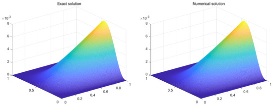
Figure 1. Comparison of the exact solutions and $P_{TAI}^{-1}\left(10\right)$ numerical solutions ($d=d_1\left(x\right)$, $\lambda =1.5$, $\beta =1.2$, ${\gamma }_1=0.75$).

Table 1. Numerical results of I, $P_{DCS}^{-1}$, $P_{SDTA{S}_{\tau }}^{-1}$, $P_{CAI}^{-1}\left(l\right)$ and $P_{TAI}^{-1}\left(l\right)$ ($d=d_1\left(x\right)$, $\lambda =1.5$, $\beta =1.2$, ${\gamma }_1=0.75$).

Method	Index	N
		${\mathbf{2}}^{\mathbf{8}}$	${\mathbf{2}}^{\mathbf{9}}$	${\mathbf{2}}^{\mathbf{10}}$	${\mathbf{2}}^{\mathbf{11}}$	${\mathbf{2}}^{\mathbf{12}}$
I	IT	87.34	108.21	123.12	134.07	140.03
	CPU	0.82	3.66	14.33	70.64	555.72
$P_{DCS}^{-1}$ [17]	$\alpha$	0.1	0.1	0.1	0.1	0.1
	IT	16.06	16.03	16.02	16.01	17.00
	CPU	0.38	1.31	4.53	17.33	65.74
$P_{SDTA{S}_{\tau }}^{-1}$ [22]	$\alpha$	0.1	0.1	0.1	0.1	0.1
	IT	11.04	12.02	14.01	15.01	16.00
	CPU	0.20	0.52	1.91	7.32	36.86
$P_{CAI}^{-1}\left(l\right)$ [25]	l	8	8	8	8	8
	IT	8.03	7.01	6.01	6.00	6.00
	CPU	0.25	0.79	2.49	9.99	37.84
${\mathit{P}}_{\mathit{TAI}}^{-\mathbf{1}}\left(\mathit{l}\right)$	l	8	8	8	8	8
	IT	6.02	5.01	5.00	5.00	4.00
	CPU	0.19	0.46	1.49	5.87	24.03

The proposed preconditioner and optimal result have been bolded.

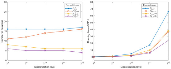
Figure 2. Comparison of average iterations and computation time for $P_{DCS}^{-1}$, $P_{SDTA{S}_{\tau }}^{-1}$, $P_{CAI}^{-1}\left(l\right)$ and $P_{TAI}^{-1}\left(l\right)$ ($d=d_1\left(x\right)$, $\lambda =1.5$, $\beta =1.2$, ${\gamma }_1=0.75$).

To further illustrate the effectiveness of the proposed preconditioning matrices, we plot the eigenvalue distributions of the original coefficient matrix A, the preconditioner $P_{DCS}^{-1}$, $P_{SDTA{S}_{\tau }}^{-1}$, $P_{CAI}^{-1}\left(l\right)$ and $P_{TAI}^{-1}\left(l\right)$ when $N={10}^8$, as shown in Figure 3. It can be observed that the eigenvalue distribution of the coefficient matrix A without preconditioning is highly dispersed, while the eigenvalue distributions of the preconditioned matrices $A{P}_{TAI}^{-1}\left(l\right)$ are concentrated around 1. Notably, the eigenvalue distribution of $A{P}_{TAI}^{-1}\left(l\right)$ is more concentrated than those of the other preconditioners.

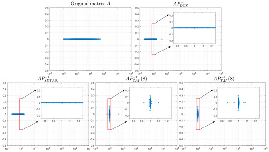
Figure 3. The eigenvalue distributions of the original coefficient matrix A, the preconditioner $P_{DCS}^{-1}$, $P_{SDTA{S}_{\tau }}^{-1}$, $P_{CAI}^{-1}\left(l\right)$ and $P_{TAI}^{-1}\left(l\right)$ ($d=d_1\left(x\right)$, $\lambda =1.5$, $\beta =1.2$, ${\gamma }_1=0.75$).

We searched for the optimal number of interpolation points l in the proposed preconditioner $P_{TAI}^{-1}\left(l\right)$. As shown in Table 2, we tested GMRES using $P_{TAI}^{-1}\left(l\right)$ with the number of interpolation points $l=4,6,8,10,12$. To determine the optimal number of interpolation points l, we visualized the number of iterations, as shown in Figure 4. By analyzing Figure 4, we found that when the number of interpolation points $l\ge 8$, the number of iterations tends to stabilize. With this observation, the number of interpolation points $l=8$ was recommended for test problem 1.

Table 2. Numerical results of $P_{TAI}^{-1}\left(l\right)$ at different numbers of interpolation points l ($d=d_1\left(x\right)$, $\lambda =1.5$, $\beta =1.2$, ${\gamma }_1=0.75$).

N	Index	Number of Interpolation Points l
		4	6	8	10	12	14
$2^8$	IT	8.03	6.02	6.02	6.02	6.02	6.02
	CPU	0.17	0.16	0.18	0.22	0.25	0.24
$2^9$	IT	8.33	5.01	5.01	5.01	5.01	5.01
	CPU	0.49	0.39	0.46	0.47	0.49	0.54
$2^{10}$	IT	8.90	5.00	5.00	5.00	5.00	5.00
	CPU	1.74	1.45	1.62	1.82	1.80	1.95
$2^{11}$	IT	9.12	6.00	5.00	5.00	5.00	5.00
	CPU	8.89	6.20	5.70	6.30	6.51	6.79
$2^{12}$	IT	10.60	5.99	4.00	4.00	4.00	4.00
	CPU	60.43	41.71	42.19	44.64	40.37	50.46

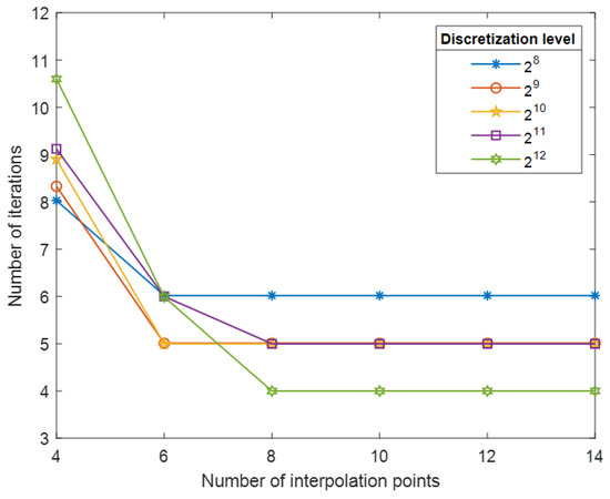
Figure 4. Number of iteration variation curves when $l=4,6,8,10,12$ ($d=d_1\left(x\right)$, $\lambda =1.5$, $\beta =1.2$, ${\gamma }_1=0.75$).

5.2. Test Problem 2

Consider the coefficient

$$d\left(x\right)={\displaystyle \frac{e^{3x}+0.2}{x\left(1-x\right)}}.$$

An illustration of the corresponding analytical solution and the numerical solution are shown in Figure 5. We compared $P_{DCS}^{-1}$, $P_{SDTA{S}_{\tau }}^{-1}$, $P_{CAI}^{-1}\left(l\right)$ and $P_{TAI}^{-1}\left(l\right)$. The results of the computations at discretization levels $N={10}^8,{10}^9,{10}^{10},{10}^{11},{10}^{12}$ are shown in Table 3 and visualized in Figure 6. In terms of the number of iterations, all preconditioning methods show relatively stable iteration numbers as the discretization level increases, but the number of iterations for $P_{TAI}^{-1}\left(l\right)$ is notably lower than that for the other three. In terms of computation time, the computation time for $P_{TAI}^{-1}\left(l\right)$ is slightly higher than that for $P_{SDTA{S}_{\tau }}^{-1}$ at discretization level $N={10}^8,{10}^9,{10}^{10}$, but the difference is not significant. As the discretization level increases, the computation time for $P_{TAI}^{-1}\left(l\right)$ grows more slowly and is significantly lower than that for the other three preconditioners. Additionally, we note that this coefficient is more complex than the last one as it has singularities at point $x=0$ and $x=1$. And this is reflected in the higher number of iterations in Table 3 and the more dispersed eigenvalue distribution in Figure 7.

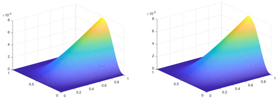
Figure 5. Comparison of the exact solutions and $P_{TAI}^{-1}\left(l\right)$ numerical solutions ($d=d_2\left(x\right)$, $\lambda =1.5$, $\beta =1.2$, ${\gamma }_1=0.75$).

Table 3. Numerical results of I, $P_{DCS}^{-1}$, $P_{SDTA{S}_{\tau }}^{-1}$, $P_{CAI}^{-1}\left(l\right)$ and $P_{TAI}^{-1}\left(l\right)$ ($d=d_2\left(x\right)$, $\lambda =1.5$, $\beta =1.2$, ${\gamma }_1=0.75$).

Method	Index	N
		${\mathbf{2}}^{\mathbf{8}}$	${\mathbf{2}}^{\mathbf{9}}$	${\mathbf{2}}^{\mathbf{10}}$	${\mathbf{2}}^{\mathbf{11}}$	${\mathbf{2}}^{\mathbf{12}}$
I	IT	125.49	174.34	233.23	300.15	∼
	CPU	1.46	7.41	46.45	225.74	∼
$P_{DCS}^{-1}$ [17]	$\alpha$	0.15	0.15	0.15	0.15	0.15
	IT	16.06	18.04	21.02	25.01	29.01
	CPU	0.48	1.52	6.14	32.83	139.03
$P_{SDTA{S}_{\tau }}^{-1}$ [22]	$\alpha$	0.15	0.15	0.15	0.15	0.15
	IT	15.06	18.04	21.02	24.01	28.01
	CPU	0.24	0.65	2.84	22.00	81.56
$P_{CAI}^{-1}\left(l\right)$ [25]	l	12	12	12	12	12
	IT	15.06	15.03	16.02	17.01	17.00
	CPU	0.49	1.60	5.42	21.00	78.15
${\mathit{P}}_{\mathit{TAI}}^{-\mathbf{1}}\left(\mathit{l}\right)$	l	12	12	12	12	12
	IT	12.05	12.02	11.01	11.01	12.00
	CPU	0.35	0.90	3.11	10.89	60.30

The proposed preconditioner and optimal result have been bolded.

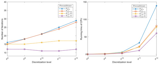
Figure 6. Comparison of average iterations and computation time for $P_{DCS}^{-1}$, $P_{SDTA{S}_{\tau }}^{-1}$, $P_{CAI}^{-1}\left(l\right)$ and $P_{TAI}^{-1}\left(l\right)$ ($d=d_1\left(x\right)$, $\lambda =1.5$, $\beta =1.2$, ${\gamma }_1=0.75$).

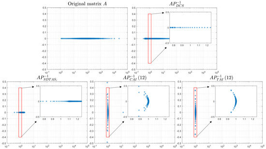
Figure 7. The eigenvalue distributions of the original coefficient matrix A, the preconditioner $P_{DCS}^{-1}$, $P_{SDTA{S}_{\tau }}^{-1}$, $P_{CAI}^{-1}\left(l\right)$ and $P_{TAI}^{-1}\left(l\right)$ ($d=d_2\left(x\right)$, $\lambda =1.5$, $\beta =1.2$, ${\gamma }_1=0.75$).

We also plot the eigenvalue distributions of A, the preconditioner $P_{DCS}^{-1}$, $P_{SDTA{S}_{\tau }}^{-1}$, $P_{CAI}^{-1}\left(l\right)$ and $P_{TAI}^{-1}\left(l\right)$ when $N={10}^8$, as shown in Figure 7. It can be observed that the eigenvalue distribution of the coefficient matrix without preconditioning is highly dispersed, while the eigenvalue distributions of the preconditioned matrices are concentrated around 1. Notably, the eigenvalue distribution of $P_{TAI}^{-1}\left(l\right)$ is more concentrated than those of the other preconditioners.

Similarly, we searched for the optimal number of interpolation points l in the proposed preconditioner $P_{TAI}^{-1}\left(l\right)$. As shown in Table 4, we tested GMRES using $P_{TAI}^{-1}\left(l\right)$ with the number of interpolation points $l=4,6,8,10,12$. To determine the optimal number of interpolation points l, we visualized the number of iterations, as shown in Figure 8. By analyzing Figure 8, we found that when the number of interpolation points $l\ge 12$, the number of iterations tends to stabilize. In this view, we selected the optimal number of interpolation points $l=12$ for the above test.

Table 4. Numerical results of $P_{TAI}^{-1}\left(l\right)$ at different numbers of interpolation points l ($d=d_2\left(x\right)$, $\lambda =1.5$, $\beta =1.2$, ${\gamma }_1=0.75$).

N	Index	Number of Interpolation Points l
		4	6	8	10	12	14
$2^8$	IT	22.09	18.07	13.05	11.04	11.04	12.05
	CPU	0.41	0.40	0.35	0.32	0.36	0.48
$2^9$	IT	25.05	21.04	12.02	11.02	12.02	12.02
	CPU	1.27	1.29	0.92	0.92	1.00	1.00
$2^{10}$	IT	27.03	15.01	13.01	11.01	11.01	12.01
	CPU	10.22	3.16	3.10	3.04	3.26	3.53
$2^{11}$	IT	31.02	16.01	14.01	11.01	12.01	11.01
	CPU	20.98	15.90	12.04	11.23	12.51	11.79
$2^{12}$	IT	60.93	34.98	14.00	13.99	12.00	13.00
	CPU	626.27	259.42	121.80	112.15	76.09	109.79

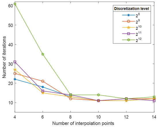
Figure 8. Number of iteration variation curves when $l=4,6,8,10,12$ ($d=d_2\left(x\right)$, $\lambda =1.5$, $\beta =1.2$, ${\gamma }_1=0.75$).

6. Concluding Remarks

In this paper, we consider solving the tempered fractional diffusion equations with variable coefficients in a numerical way. The problem is discretized by the Crank–Nicolson method and the tempered weighted and shifted Grünwald formula. For the resulting linear system, we approximate the SPD Toeplitz matrix by the $\tau$ matrix and take the advantage of the row-by-row approximation strategy to construct an approximate inverse preconditioner. A spectral analysis reveals that the eigenvalues of the preconditioned system matrix are tightly clustered near unity. Experiments further validate the enhanced convergence enabled by the developed preconditioner.

References

- Baeumer, B.; Meerschaert, M.M. Tempered stable Lévy motion and transient super-diffusion. J. Comput. Appl. Math. 2010, 233, 2438–2448. [Google Scholar] [CrossRef]
- Magin, R.L. Fractional calculus in bioengineering. Crit. Rev. Biomed. Eng. 2004, 32, 1–104. [Google Scholar] [CrossRef]
- Meerschaert, M.M.; Zhang, Y.; Baeumer, B. Tempered anomalous diffusion in heterogeneous systems. Geophys. Res. Lett. 2008, 35, L17403. [Google Scholar] [CrossRef]
- Zhang, H.; Liu, F.; Turner, I.; Chen, S. The numerical simulation of the tempered fractional Black-Scholes equation for European double barrier option. Appl. Math. Model. 2016, 40, 5819–5834. [Google Scholar] [CrossRef]
- Huang, X.; Sun, H.-W. A preconditioner based on sine transform for two-dimensional semi-linear Riesz space fractional diffusion equations in convex domains. Appl. Numer. Math. 2021, 169, 289–302. [Google Scholar] [CrossRef]
- Qin, H.; Pang, H.; Sun, H. Sine transform based preconditioning techniques for space fractional diffusion equations. Numer. Linear Algebra Appl. 2023, 30, e2474. [Google Scholar] [CrossRef]
- Sun, L.-Y.; Lei, S.-L.; Sun, H.-W.; Zhang, J.-L. An α-robust fast algorithm for distributed-order time–space fractional diffusion equation with weakly singular solution. Math. Comput. Simul. 2023, 207, 437–452. [Google Scholar] [CrossRef]
- Zhang, C.-H.; Yu, J.-W.; Wang, X. A fast second-order scheme for nonlinear Riesz space-fractional diffusion equations. Numer. Algorithms 2023, 92, 1813–1836. [Google Scholar] [CrossRef]
- Liu, J.; Fu, H.; Wang, H.; Chai, X. A preconditioned fast quadratic spline collocation method for two-sided space-fractional partial differential equations. J. Comput. Appl. Math. 2019, 360, 138–156. [Google Scholar] [CrossRef]
- Lu, X.; Fang, Z.-W.; Sun, H.-W. Splitting preconditioning based on sine transform for time-dependent Riesz space fractional diffusion equations. J. Appl. Math. Comput. 2021, 66, 673–700. [Google Scholar] [CrossRef]
- Shao, X.-H.; Kang, C.-B. A preconditioner based on sine transform for space fractional diffusion equations. Appl. Numer. Math. 2022, 178, 248–261. [Google Scholar] [CrossRef]
- Qu, W.; Liang, Y. Stability and convergence of the Crank-Nicolson scheme for a class of variable-coefficient tempered fractional diffusion equations. Adv. Differ. Equ. 2017, 2017, 108. [Google Scholar] [CrossRef]
- Wang, W.; Chen, X.; Ding, D.; Lei, S.-L. Circulant preconditioning technique for barrier options pricing under fractional diffusion models. Int. J. Comput. Math. 2015, 92, 2596–2614. [Google Scholar] [CrossRef]
- Li, C.; Deng, W. High order schemes for the tempered fractional diffusion equations. Adv. Comput. Math. 2016, 42, 543–572. [Google Scholar] [CrossRef]
- Serra, S. Superlinear PCG methods for symmetric Toeplitz systems. Math. Comput. 1999, 68, 793–803. [Google Scholar] [CrossRef]
- Wang, C.; Li, H.; Zhao, D. Preconditioning Toeplitz-plus-diagonal linear systems using the Sherman-Morrison-Woodbury formula. J. Comput. Appl. Math. 2017, 309, 312–319. [Google Scholar] [CrossRef]
- Bai, Z.-Z.; Lu, K.-Y.; Pan, J.-Y. Diagonal and Toeplitz splitting iteration methods for diagonal-plus-Toeplitz linear systems from spatial fractional diffusion equations. Numer. Linear Algebra Appl. 2017, 24, e2093. [Google Scholar] [CrossRef]
- Wang, C.; Li, H.; Zhao, D. Improved block preconditioners for linear systems arising from half-quadratic image restoration. Appl. Math. Comput. 2019, 363, e124614. [Google Scholar] [CrossRef]
- Lei, S.; Fan, D.; Chen, X. Fast solution algorithms for exponentially tempered fractional diffusion equations. Numer. Methods Partial Differ. Equ. 2018, 34, 1301–1323. [Google Scholar] [CrossRef]
- Zhao, Y.-L.; Zhu, P.-Y.; Gu, X.-M.; Zhao, X.-L.; Jian, H.-Y. A preconditioning technique for all-at-once system from the nonlinear tempered fractional diffusion equation. J. Sci. Comput. 2020, 83, 10. [Google Scholar] [CrossRef]
- Qu, W.; Lei, S.-L. On CSCS-based iteration method for tempered fractional diffusion equations. Jpn. J. Ind. Appl. Math. 2016, 33, 583–597. [Google Scholar] [CrossRef]
- Tang, S.-P.; Huang, Y.-M. A matrix splitting preconditioning method for solving the discretized tempered fractional diffusion equations. Numer. Algorithms 2023, 92, 1311–1333. [Google Scholar] [CrossRef]
- Feng, Y.; Zhang, X.; Chen, Y.; Wei, L. A compact finite difference scheme for solving fractional Black-Scholes option pricing model. J. Inequal. Appl. 2025, 2025, 36. [Google Scholar] [CrossRef]
- Zhang, X.; Wei, L.; Liu, J. Application of the LDG method using generalized alternating numerical flux to the fourth-order time-fractional sub-diffusion model. Appl. Math. Lett. 2025, 168, 109580. [Google Scholar] [CrossRef]
- Pan, J.; Ke, R.; Ng, M.K.; Sun, H.-W. Preconditioning techniques for diagonal-times-Toeplitz matrices in fractional diffusion equations. SIAM J. Sci. Comput. 2014, 36, A2698–A2719. [Google Scholar] [CrossRef]
- Chou, L.-K.; Lei, S.-L. Fast ADI method for high dimensional fractional diffusion equations in conservative form with preconditioned strategy. Comput. Math. Appl. 2017, 73, 385–403. [Google Scholar] [CrossRef]
- Du, N.; Sun, H.-W.; Wang, H. A preconditioned fast finite difference scheme for space-fractional diffusion equations in convex domains. Comput. Appl. Math. 2019, 38, 14. [Google Scholar] [CrossRef]
- Gan, D.; Zhang, G.-F. Efficient ADI schemes and preconditioning for a class of high-dimensional spatial fractional diffusion equations with variable diffusion coefficients. J. Comput. Appl. Math. 2023, 423, 114938. [Google Scholar] [CrossRef]
Disclaimer/Publisher’s Note: The statements, opinions and data contained in all publications are solely those of the individual author(s) and contributor(s) and not of MDPI and/or the editor(s). MDPI and/or the editor(s) disclaim responsibility for any injury to people or property resulting from any ideas, methods, instructions or products referred to in the content. |
© 2025 by the authors. Licensee MDPI, Basel, Switzerland. This article is an open access article distributed under the terms and conditions of the Creative Commons Attribution (CC BY) license (https://creativecommons.org/licenses/by/4.0/).