Combining the A* Algorithm with Neural Networks to Solve the Team Orienteering Problem with Obstacles and Environmental Factors

Abstract

This paper addresses the team orienteering problem applied to unmanned aerial vehicles (UAVs), considering obstacle avoidance and environmental factors such as wind conditions and payload weight. The objective is to optimize UAV routes to maximize collected rewards while adhering to operational constraints. To achieve this, we employ a simheuristic algorithm for the overall route optimization, while integrating the A* algorithm to determine feasible paths between nodes that avoid obstacles in a 2D grid-based environment. Then, a feedforward neural network estimates travel time based on UAV speed, wind conditions, trajectory distance, and payload weight. This estimation is incorporated into the optimization process to improve route planning accuracy. Numerical experiments evaluate the impact of various parameters, including obstacle placement, UAV speed, wind conditions, and payload weight. These experiments include maps with 30 to 100 points of interest and varying obstacle densities and show that our hybrid method improves solution quality by up to $15\%$ in total profit compared to a baseline approach. Furthermore, computation times remain within 5–10% of the baseline, showing that the added predictive layer maintains computational efficiency.

1. Introduction

The team orienteering problem (TOP) is a combinatorial optimization problem that involves selecting a subset of locations, each associated with a specific reward [1,2,3]. The goal is to plan routes for a team of agents to maximize the total collected reward while satisfying operational constraints. These constraints may include time limits, agent capacities, and the structure of the route network [4,5,6]. The TOP belongs to the class of orienteering problems [7] and has applications in healthcare logistics [8], tourism [9], and resource management, where optimizing the use of limited resources is essential [10]. In the TOP, each agent must determine not only which locations to visit but also the optimal sequence to maximize total reward while adhering to imposed constraints. These characteristics increase the problem’s difficulty, as both node selection and visit sequence are crucial for optimization.

This study extends the traditional TOP framework by applying it to a fleet of unmanned aerial vehicles (UAVs). In addition to standard constraints, we incorporate environmental factors such as obstacles and wind conditions, which influence UAV performance. To compute routes that avoid obstacles, we employ the A* algorithm, a widely used path-planning method for UAVs [11,12]. Hence, this paper addresses the scientific problem of solving the TOP under realistic constraints (e.g., physical obstacles and environmental conditions) that are typically ignored in classical approaches. These factors significantly affect the feasibility and efficiency of routes, particularly in applications involving UAVs or autonomous vehicles.

The problem is modeled on a two-dimensional grid map, allowing a precise representation of the environment. Using A*, we efficiently determine paths that minimize travel distance while ensuring obstacle avoidance. Once a path is established, the UAV’s travel time is estimated based on several factors. The trajectory between two locations is defined as a sequence of two-dimensional coordinates obtained using A*. The total travel distance is computed as the sum of Euclidean distances between successive coordinates, measured in kilometers. The estimated travel time considers: (i) the UAV’s speed, assumed to be constant along the trajectory; (ii) the wind’s speed and direction, which influence the UAV’s effective speed; and (iii) the weight of onboard sensors and equipment required for operations at each location.

Figure 1 shows two trajectories: one from node 1 to node 2 and another from node 2 to node 3. These trajectories are located on a 30 × 30 km grid. The following factors influence the UAV’s trajectory: (i) UAV speed—the UAV maintains a constant speed along the entire trajectory (km/min); (ii) wind speed and direction—wind velocity (km/min) and direction (radians) are considered as environmental factors, which can increase or decrease the UAV’s effective speed depending on the trajectory; and (iii) payload weight—the weight (kg) of sensor equipment and other devices mounted on the UAV, which are necessary for performing operations at each location.

To predict travel time, we employed a multi-layer fully connected feedforward neural network [13], suitable for regression tasks. The network’s input features include (i) UAV speed; (ii) distance between two trajectory coordinates; (iii) angle between successive trajectory vectors; (iv) wind speed and direction; and (v) payload weight. For multi-coordinate trajectories, the network estimates the travel time between each successive coordinate pair, and the total time is obtained by summing these individual estimates. With this time estimation model, we can solve the TOP by optimizing UAV routes using the A* algorithm.

Figure 2 illustrates a simplified example of a TOP solution on a 30 × 30 km grid, where two UAVs plan their routes to maximize collected rewards while avoiding obstacles: (i) nodes are represented as numbered blue circles, with larger circles indicating higher rewards; (ii) the first UAV follows the yellow path, starting from node 1 (red square) and visiting nodes 7, 11, 10, 5, 9, and 12; (iii) the second UAV follows the purple path, also starting from node 1 and visiting nodes 4, 8, 6, and 12; (iii) obstacles appear as black rectangles, requiring UAVs to adjust their routes accordingly; and (iv) a red arrow in the top-right corner represents wind direction and speed (18 km/h), a key environmental factor in trajectory optimization.

The main contributions of this study are described as follows: (i) we extend the classical TOP by integrating obstacle avoidance and environmental factors, including wind speed, wind direction, and payload weight, which impact UAV performance; (ii) the A* algorithm is applied to determine the shortest path between nodes, ensuring UAVs navigate complex environments while avoiding obstacles; (iii) a feedforward neural network is used to estimate UAV travel time, incorporating UAV speed, trajectory distance, wind conditions, and payload; and (iv) we analyze the impact of various parameters, including obstacle size and position, maximum nodes per route, route duration, UAV speed, wind conditions, and payload weight. Hence, the novelty of this approach lies in combining classical A*-based path-finding with a data-driven model to account for real-time environmental effects on UAV mobility, an aspect not typically addressed in the standard TOP literature. Theoretical contributions involve expanding the classical TOP framework to account for spatial constraints and dynamic variables, while the practical significance is shown in its potential applications to UAV logistics, disaster response, and environmental monitoring.

The remainder of this paper is structured as follows: Section 2 reviews related work on TOP and UAV-based path planning. Section 3 presents the problem formulation and modeling approach. Section 4 details the proposed methodology, including A*-based path planning and neural network time estimation. Section 5 discusses experimental results, and Section 6 concludes with insights and future research directions.

2. Related Work

The dynamic TOP [14] with obstacles, introduced in this paper, represents a significant advancement in rich and real-life logistics, integrating environmental dynamics and physical constraints into the classical TOP. This section reviews state-of-the-art methodologies, identifying key gaps and positioning the novelty of this study within the existing literature.

Heuristic and metaheuristic approaches have proven effective in addressing the computational challenges of the TOP. Methods such as iterated local search (ILS) have significantly improved solution quality, particularly in dynamic and constrained environments [15,16]. These methods optimize node selection and route sequencing, efficiently delivering near-optimal solutions. Simulated annealing (SA) has also been employed to tackle the TOP and its variants. Enhancements in SA-based heuristics have successfully optimized multi-objective formulations of the problem [17,18], while effective in static scenarios, these techniques have limited adaptability to dynamic conditions.

Stochastic extensions of the TOP, such as the stochastic team orienteering problem (STOP), introduce uncertainty in travel times and rewards. Methods like simheuristics, which combine Monte Carlo simulation with traditional heuristics, have been used to manage variability effectively [6]. These techniques enable UAV route optimization under uncertainty, making them useful in applications such as surveillance and emergency response. Further advancements have addressed dynamic environments by integrating weather conditions and real-time changes in rewards. Works focusing on weather-adaptive routing highlight the influence of environmental factors on UAV performance [19,20]. However, these studies often lack explicit modeling physical obstacles, limiting their applicability in complex operational scenarios.

The team assignment orienteering problem (TAOP) extends the classical TOP by incorporating task-specific requirements and stochastic constraints. Studies on task allocation for UAV fleets have developed strategies to optimize both task assignment and route planning [21,22]. These approaches use coordination mechanisms to ensure efficient coverage and reward maximization. Simheuristics and learnheuristics [23,24] have also been applied to manage stochasticity and dynamism in task assignment and routing, particularly in applications involving heterogeneous fleets [25]. However, these methods rarely address dynamic obstacles or integrate predictive modeling for travel times.

Recent studies emphasize the need to account for environmental and physical constraints in TOP solutions. Research addressing UAV battery limitations and weather impacts has demonstrated significant efficiency improvements [26,27], while valuable, these advancements often simplify obstacle representation, limiting their utility in real-world scenarios.

Despite progress in TOP research, several critical gaps remain: (i) few approaches explicitly incorporate obstacles, a critical component in real-world UAV routing [19,20]; (ii) limited work has utilized machine learning for travel time predictions in dynamic scenarios; and (iii) balancing reward maximization with dynamic environmental factors remains underexplored. Our work addresses these gaps through modeling of physical obstacles using the A* algorithm for safe and efficient routing and a feedforward neural network predicts travel times, incorporating factors like wind speed, UAV load, and obstacle density.

3. Problem Formulation

The mathematical model of our problem is based on the one proposed by Chao et al. [1] for the TOP. In this study, we manage a fleet $D=\{1,2,\dots ,d\}$ consisting of d homogeneous UAVs. Each UAV aims to visit as many nodes as possible within a specified time limit, starting at an initial node and ending at a final node. Upon visiting a node, a UAV receives a corresponding reward, and no other UAV can collect the reward from the same node. Thus, each team member must select a subset of nodes to visit, minimizing overlap among UAVs while complying with time constraints and maximizing the team’s total score. The TOP is formalized within a directed graph $G=(V,A)$, where (i) the set of nodes is $V=\{0,1,2,\dots ,n\}$, with node 0 representing the initial depot and node n representing the final depot; (ii) the set of arcs is defined as $A=\left\{\right(i,j)\mid i,j\in V,i\ne j\}$; and (iii) the set of rewards is $R=\{r_0,r_1,r_2,\dots ,r_n\}$, where $r_i>0$ is the reward a UAV receives when visiting node i.

Each UAV $d\in D$ starts its route at the initial depot, visits several intermediate nodes, and ends at the final depot. This implies that the maximum number of routes in any solution equals the fleet size D. The travel time between nodes i and j is denoted by $T_{ij}>0$ (if $i\ne j$), and the parameter $t_{max}>0$ represents the maximum allowed duration for a route. It is important to note that rewards are accumulated only the first time a node is visited, i.e., revisiting a node does not grant additional benefits. The objective is to maximize the total sum of rewards obtained by all UAVs.

To model the problem, we define the following binary variables: $y_{id}$ takes the value 1 if node $i\in V$ is visited by UAV $d\in D$, and 0 otherwise; $x_{ijd}$ takes the value 1 if arc $(i,j)$ is traversed by UAV $d\in D$, and 0 otherwise. Under these conditions, the goal is to maximize the total collected reward:

$$max\sum _{d\in D}\sum _{i\in V}{r}_i{y}_{id}$$

(1)

In addition, the following constraints apply:

If a node i is visited, there must exist an arc connecting it, as follows:

$$\sum _{j\in V,j\ne i}{x}_{ijd}=y_{id},\forall i\in V,d\in D$$

(2)

The initial and final depots should not be visited by more UAVs than the fleet size:

$$\sum _{d\in D}{y}_{0d}\le \left|D\right|,\sum _{d\in D}{y}_{nd}\le \left|D\right|$$

(3)

Each intermediate node i must be visited by only one UAV:

$$\sum _{d\in D}{y}_{id}\le 1,\forall i\in V\setminus \{0,n\}$$

(4)

The total travel time of any UAV must not exceed $t_{max}$:

$$\sum _{(i,j)\in A}{T}_{ij}{x}_{ijd}\le t_{max},\forall d\in D$$

(5)

The variables $y_{id}$ and $x_{ijd}$ must be binary:

$$y_{id}\in \{0,1\},x_{ijd}\in \{0,1\},\forall i,j\in V,d\in D$$

(6)

It is important to note that in real-world UAV operations, travel times between nodes are often subject to uncertainty due to environmental factors. In our model, we consider this uncertainty by classifying edges into deterministic and stochastic categories. Specifically, edges whose end node has an even ID ($i\in V$ where $imod2=0$) or is divisible by three ($imod3=0$) are considered to have stochastic travel times, while the remaining edges have deterministic travel times. This classification allows us to model realistic scenarios where travel time variability may affect route feasibility and reward collection.

4. Solution Method

In this section, the solving methodology is provided. We will first describe the methodology, in general, and then we will provide details on the ‘real-value’ computation of the travel time as well as on its estimation using a neural network.

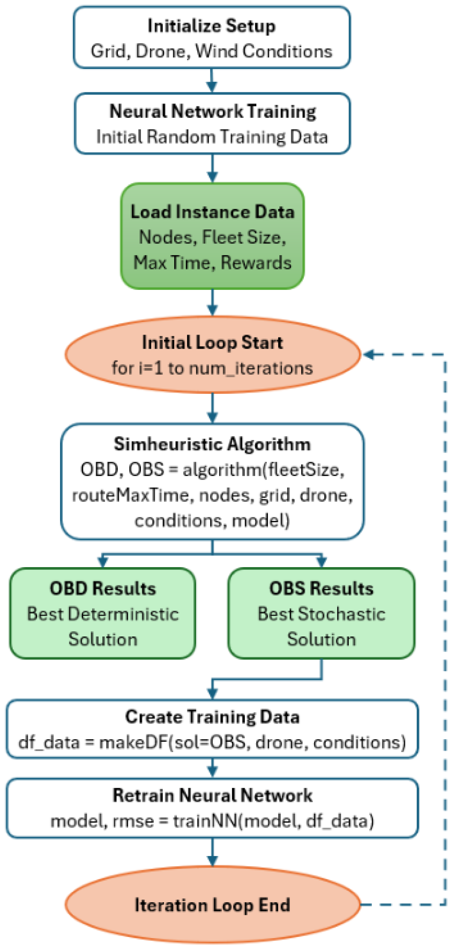
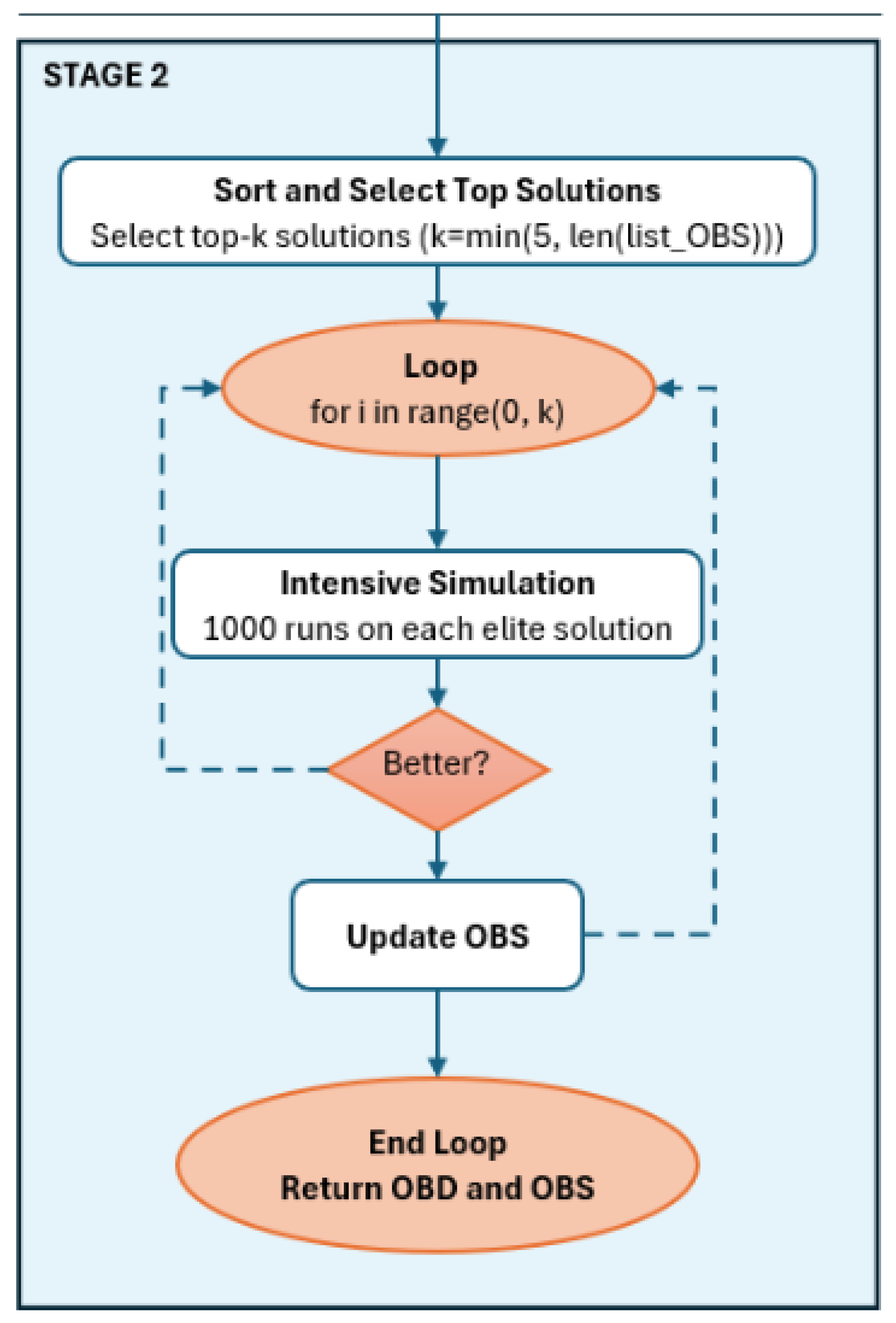
4.1. Overview of Our Approach

Our approach starts with an initialization phase that has two main parts (Figure 3). First, the ‘Initial Setup’ creates the environment for UAV route planning by configuring a grid-based operational area and placing obstacles. It also sets the drone’s speed and payload capacity and defines environmental conditions like wind speed and direction. After setting up the environment, the system trains a neural network with random data to create an initial predictive model. This model estimates travel times based on factors like UAV speed, distance, wind conditions, and payload weight. Using synthetic data for various scenarios, it establishes a foundation for accurate predictions before actual route planning. The travel time estimates will be refined through feedback as more operational data are collected.

After initialization, the system loads instance data from input files detailing problem specifications. Each file includes parameters like the number of nodes (UAV points), fleet size (number of UAVs), and maximum route duration. The system extracts node locations and rewards, ensuring they do not conflict with obstacles. This converts raw descriptions into structured data for route planning algorithms, defining the optimization challenge. At the core of our methodology lies an iterative optimization and learning process. Each iteration executes our simheuristic algorithm to generate two solutions: OBD (our best deterministic solution) and OBS (our best stochastic solution). The system then extracts operational data from the OBS to retrain the neural network model, improving travel time prediction accuracy. This feedback loop between optimization and learning represents a key innovation—the system progressively learns from its own results, creating increasingly reliable UAV routing solutions with each iteration. Rather than treating travel time estimation as static, we continuously refine it throughout the solution process, enhancing route quality as the neural network adapts to operational realities.

The simheuristic algorithm follows a two-stage approach to solve the dynamic team-orienteering problem with obstacles. The process begins with an initialization phase that creates an initial solution by setting the alpha value for enhanced savings calculations and generating an initial efficiency list. This solution is established as our initial best deterministic solution (OBD) and serves as the first entry in our list of candidate solutions. Stage 1 focuses on building a collection of high-quality candidate solutions through an iterative time-constrained process (Figure 4). During this stage, the algorithm repeatedly generates new solutions using a merging process with biased randomization. Each promising solution (one that exceeds the current best reward) is designated as the new OBD and undergoes Monte Carlo simulation with 100 runs to evaluate its performance under stochastic conditions. These promising solutions are added to the list of candidate stochastic solutions (${\mathrm{list}}_{O}BS$). This stage efficiently explores the solution space to identify diverse high-quality route configurations that perform well under varying conditions.

As shown in Figure 5, Stage 2 refines the most promising stochastic solutions to determine our best stochastic solution (OBS). First, the algorithm sorts all candidate solutions in ${\mathrm{list}}_{O}BS$ by their simulated reward values and selects the top-k solutions, where k is the minimum between a predefined maximum (5) and the total number of candidates. Each of these elite solutions undergoes a more intensive Monte Carlo simulation with 1000 runs to more accurately assess its performance under uncertainty. The solution that demonstrates the highest reward after this intensive simulation becomes the final OBS.

This two-stage approach balances exploration and refinement, efficiently identifying solutions that not only maximize rewards in deterministic settings but also maintain robustness when facing the uncertainties inherent in real-world UAV operations with varying environmental conditions.

To account for uncertainty in travel times, our simheuristic algorithm incorporates a Monte Carlo simulation module. This module evaluates candidate solutions under stochastic conditions, providing a more realistic assessment of solution quality in uncertain environments. Each promising deterministic solution undergoes multiple simulation runs to estimate its expected performance when travel times vary according to predefined probability distributions.

A critical aspect of our methodology lies in the integration of the A* algorithm and neural network predictive modeling during the solution generation process. As illustrated in Figure 6, for each potential edge between nodes in our problem, we employ a two-step approach to determine both the optimal route and its expected travel time. First, the A* algorithm calculates the optimal path between nodes while ensuring obstacle avoidance. Operating on our 2D grid-based environment representation, A* efficiently explores the state space to determine the shortest feasible path between any two nodes. This process is essential for ensuring UAV routes remain physically viable in environments with obstacles. Simultaneously, our neural network model predicts the travel time for each path segment. The network takes as input multiple features including UAV speed, path distance, trajectory angles, wind conditions (speed and direction), and payload weight. These predictions account for the complex interplay of environmental factors that impact UAV performance beyond mere distance considerations.

The integration of these components occurs for every potential edge in our solution space: both between intermediate nodes and between nodes and depot locations. The best-found paths and their predicted travel times are stored in an efficiency list, which serves as the foundation for our merging process during solution generation. This approach ensures that all routes generated by our simheuristic algorithm are not only feasible regarding obstacle avoidance but also accurately reflect expected travel times under varying environmental conditions.

4.2. Black-Box Modeling of UAV Travel Time on an Arc

In the context of the routing problem, determining the time required for a UAV to traverse an arc $(i,j)$ is key for ensuring route feasibility. This calculation involves multiple interacting factors, including UAV speed, wind conditions, payload weight, and arc geometry. These factors interact in a nonlinear and context-dependent manner. Due to this complexity, we treat this calculation as a ‘black box’ (emulation of reality), whose exact behavior is not directly accessible by the algorithm but is based on the following principles.

The UAV’s initial speed $v_{\mathrm{drone}}$ is reduced as a function of the payload weight $w_{\mathrm{payload}}$. This reduction follows a nonlinear relationship proportional to the square of the payload weight:

$$v_{\mathrm{adjusted}}=v_{\mathrm{drone}}-(k·w_{\mathrm{payload}}^2)$$

(7)

where k is a coefficient that captures the impact of weight on speed.

Wind conditions, both in magnitude and direction $(v_{\mathrm{wind}},{\theta }_{\mathrm{wind}})$, significantly affect the UAV’s effective speed when traversing an arc $(i,j)$. These effects are modeled by considering the vector components of both the wind and the UAV:

$$v_{\mathrm{resultant}}=\sqrt{{(v_{\mathrm{drone},x}+v_{\mathrm{wind},x})}^2+{(v_{\mathrm{drone},y}+v_{\mathrm{wind},y})}^2}$$

(8)

where

$$\begin{array}{cc}\hfill v_{\mathrm{drone},x}& =v_{\mathrm{adjusted}}·cos\left({\theta }_{\mathrm{path}}\right)\hfill \end{array}$$

(9)

$$\begin{array}{cc}\hfill v_{\mathrm{drone},y}& =v_{\mathrm{adjusted}}·sin\left({\theta }_{\mathrm{path}}\right)\hfill \end{array}$$

(10)

and

$$\begin{array}{cc}\hfill v_{\mathrm{wind},x}& =v_{\mathrm{wind}}·cos\left({\theta }_{\mathrm{wind}}\right)\hfill \end{array}$$

(11)

$$\begin{array}{cc}\hfill v_{\mathrm{wind},y}& =v_{\mathrm{wind}}·sin\left({\theta }_{\mathrm{wind}}\right)\hfill \end{array}$$

(12)

The arc $(i,j)$ is decomposed into smaller segments, and for each segment, the Euclidean distance and required time are computed based on the resultant ground speed.

$$t_{\mathrm{segment}}={\displaystyle \frac{d_{\mathrm{segment}}}{v_{\mathrm{resultant}}}}$$

(13)

The total travel time for an arc is the sum of the travel times for all its segments.

$$T_{ij}=\sum _k{t}_{\mathrm{segment},k}$$

(14)

4.3. A White-Box Neural Network Approach for Travel Time Estimation

The proposed neural network does not estimate the total trajectory time directly. Instead, it calculates the travel time for each segment, summing them to obtain the total time. This modular approach efficiently handles dynamic conditions and nonlinear interactions. The network takes six input features describing the arc and UAV conditions: UAV speed $v_{\mathrm{drone}}$, segment distance d, segment direction angle ${\theta }_{\mathrm{dist}}$, wind speed $v_{\mathrm{wind}}$, wind direction ${\theta }_{\mathrm{wind}}$, payload weight $w_{\mathrm{payload}}$.

The network consists of three fully connected hidden layers (Figure 7): layer 1 with 64 neurons, layer 2 with 64 neurons, and layer 3 with 32 neurons. Each layer uses the ReLU activation function to introduce nonlinearity. The final layer produces a single value representing the estimated travel time for the segment. The network contains approximately $64,000$ parameters, balancing learning capacity and computational efficiency. For each segment in an A*-generated path, the actual travel time is computed using the physical model. The dataset includes UAV speed, segment distance, angles, wind conditions, and payload weight.

The neural network was trained using a carefully designed process to ensure a balance between accuracy and efficiency. Data preprocessing involved standard normalization and an $80/20$ train-test split, with no additional feature engineering. The model was trained using the Adam optimizer with a learning rate of $0.001$, a batch size of 10, and early stopping based on validation loss. The training was conducted on a PyTorch (https://pytorch.org/) setup with an Intel Core i7-1280P processor, requiring under 1 GB of RAM and taking about 2 to 3 min per full training cycle for larger datasets. An iterative refinement strategy was applied, where the model was initially trained on synthetic data, then progressively retrained with added examples based on discrepancies between predicted and simulated travel times. For a 21-node problem instance, stable performance was typically reached after 20 to 30 iterations, with RMSE improving from $0.70$ to $0.40$ or lower, and in some cases as low as $0.22$. Even after 5 to 10 iterations, the model achieved sufficient accuracy for practical route planning. The average computational time per iteration—including path generation, simulation, and training—was approximately 65 s on the test hardware.

The neural network is progressively refined using an iterative approach combining simulation, real-time comparisons, and retraining. The iterative process is described as follows: (i) generate deterministic and stochastic solutions (OBD and OBS) using the trained neural network; (ii) simulate real travel times using the physical model; (iii) compare estimated and real travel times to identify discrepancies; (iv) use discrepancies to generate new training data; (v) retrain the network to minimize RMSE; and (vi) update solutions with refined travel time estimates. As it will be discussed in the experimental section, the proposed model handles dynamically generated trajectories. It learns complex patterns and applies them to new conditions. Once trained, the model rapidly predicts segment travel times, improving overall system performance.

4.4. Modeling Travel Time Uncertainty

To model the stochasticity in UAV travel times, we classify each edge $(i,j)$ in the solution according to the characteristics of its end node j. Edges connecting to nodes with even IDs or IDs divisible by three are designated as stochastic, while all other edges maintain deterministic travel times. This assignment is formalized as follows:

$$\text{edge\_type}(i,j)=\left\{\begin{array}{cc}1\left(\mathrm{stochastic}\right),\hfill & \mathrm{if}jmod2=0\mathrm{or}jmod3=0\hfill \\ 0\left(\mathrm{deterministic}\right),\hfill & \mathrm{otherwise}\hfill \end{array}\right.$$

(15)

For edges with stochastic travel times, we employ a lognormal distribution with a variance level parameter $\lambda =0.3$. The mean parameter $\mu$ of this distribution is set to the travel time predicted by our neural network model, establishing a direct connection between our predictive framework and the stochastic simulation. This parameter represents a moderate level of variability and was chosen based on empirical observations of UAV operations in semi-controlled environments. Given a mean travel time $\mu$, we derive the parameters of the lognormal distribution as follows:

$${\sigma }^2=0.3·\mu \left(\mathrm{variance}\right)$$

(16)

$${\mu }^{\prime }=ln\left({\displaystyle \frac{{\mu }^2}{\sqrt{{\sigma }^2+{\mu }^2}}}\right)(\log -\mathrm{mean})$$

(17)

$${\sigma }^{\prime }=\sqrt{ln\left(1+{\displaystyle \frac{{\sigma }^2}{{\mu }^2}}\right)}(\log -\mathrm{standard}\mathrm{deviation})$$

(18)

The travel time for a stochastic edge is then sampled from $\mathrm{lognormal}({\mu }^{\prime },{\sigma }^{\prime })$. This approach allows us to model realistic variations in travel times while maintaining computational tractability.

During the Monte Carlo simulation phase, each candidate solution is evaluated across multiple runs (100 for the initial assessment and 1000 for the final refinement). For each run, the travel times of stochastic edges are randomly sampled from their respective distributions. If the total travel time of a route exceeds the maximum allowed duration, the entire reward for that route is forfeited, reflecting the operational reality that incomplete missions yield no benefit.

5. Numerical Experiments and Analysis of Results

The proposed methodology was developed entirely in Python 3.12.7, using key libraries such as NumPy (2.2.3) for numerical operations, PyTorch (2.6.0) for neural network implementation, scikit-learn (1.6.1) for evaluation metrics, and Matplotlib (3.10.1) for visualizations. These tools supported the implementation of the A* algorithm, the feedforward neural network for travel time estimation, and the simulation of UAV routing scenarios with obstacles and environmental factors, resulting in a fully Python-based solution without the need for external software. The computational experiments were conducted on a computer with a 12th Generation Intel^® Core^TM $i7$-1280P processor at $1.80$ GHz, 32 GB RAM, and running Windows 11 Pro (version 24H2) 64-bit. Due to the absence of standardized benchmarks for the dynamic TOP with obstacles, a diverse set of synthetic test instances was developed. These instances were designed to reflect the complexities inherent in realistic UAV routing scenarios, integrating various operational and environmental constraints. All experiments were conducted on a $30\times 30$ km grid-based environment.

Two primary instance sets were created to evaluate the proposed approach: one comprising 21 nodes and another with 31 nodes. For each instance set, scenarios with and without obstacles were considered to assess the impact of obstacle avoidance on route optimization. Figure 8 illustrates the spatial distribution of nodes, obstacles, and depots for both instance sets.

The experimental framework was structured to systematically evaluate the influence of critical parameters:

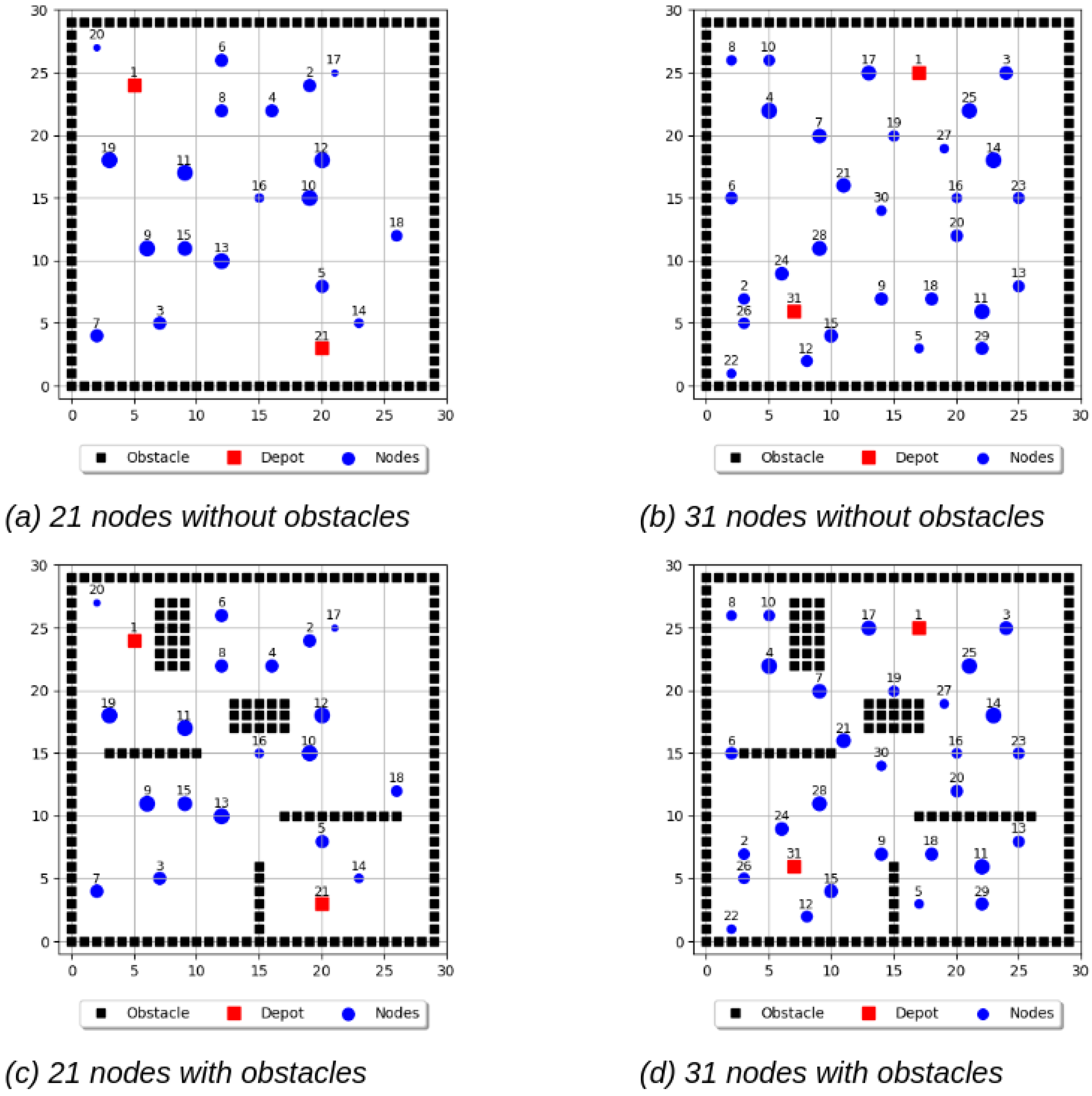
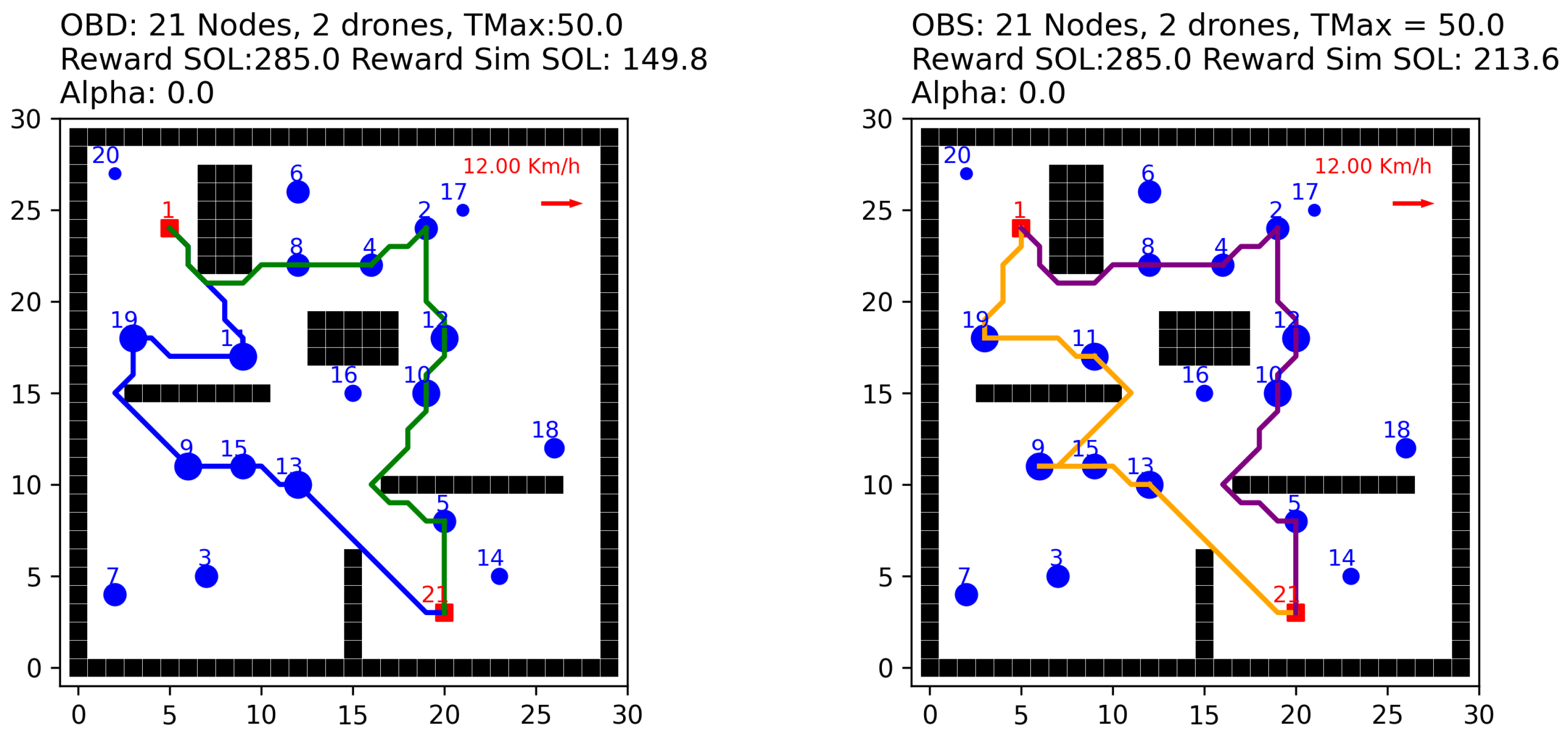
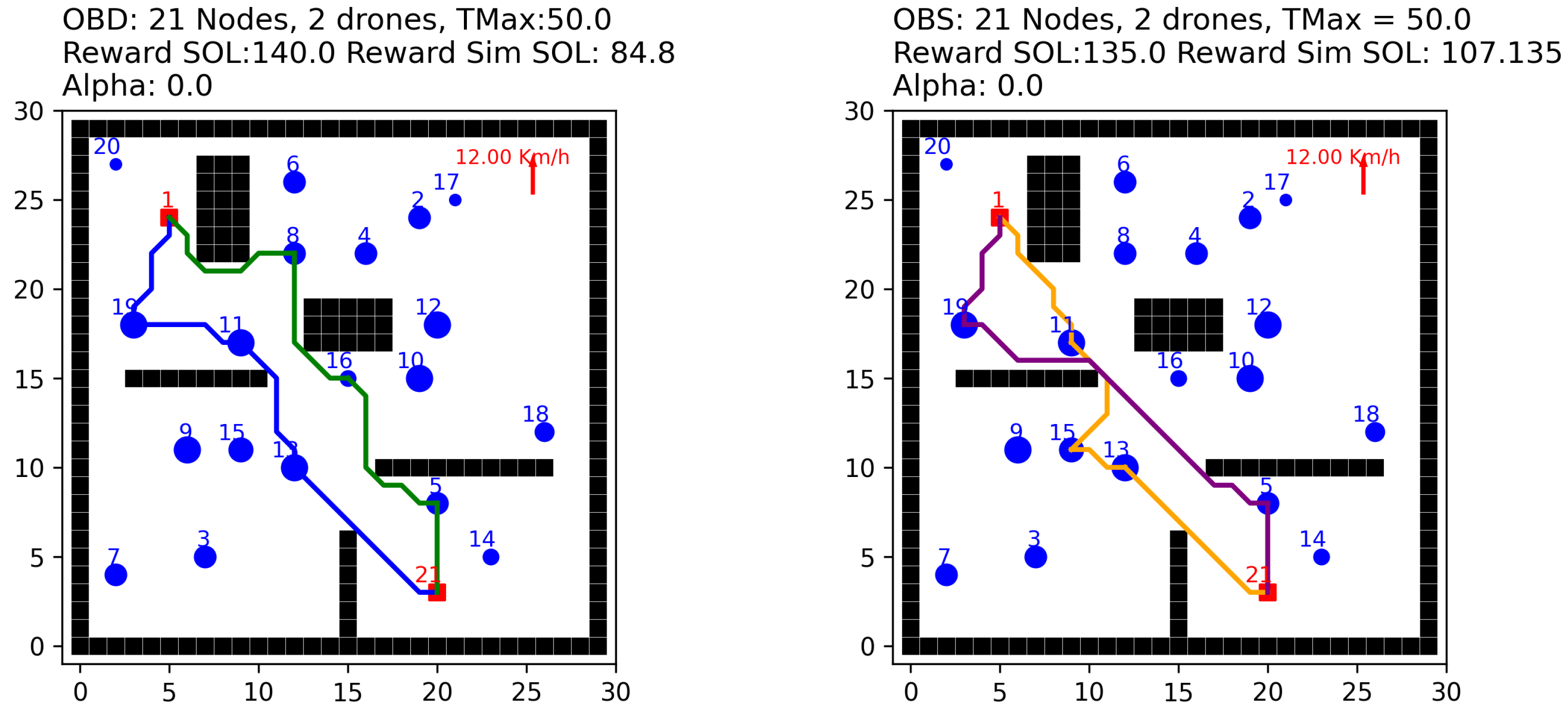
• Obstacle configuration: Two scenarios were tested, obstacle-free environments and environments with strategically placed obstacles that UAVs must avoid.
• Wind conditions: Wind speed was varied between 0 km/min (no wind) and $0.3$ km/min, with directional variations at $0^{\circ }$, ${90}^{\circ }$, ${180}^{\circ }$, and ${270}^{\circ }$.
• Payload weight: Tests were conducted with payloads of 0 kg (no payload) and 1 kg.
• UAV travel speed: Two different UAV speeds were examined, $0.8$ km/min and $1.1$ km/min.
• Route duration limitations: Maximum route durations of 36 min and 46 min were imposed, reflecting typical operational constraints in real-world UAV deployments.

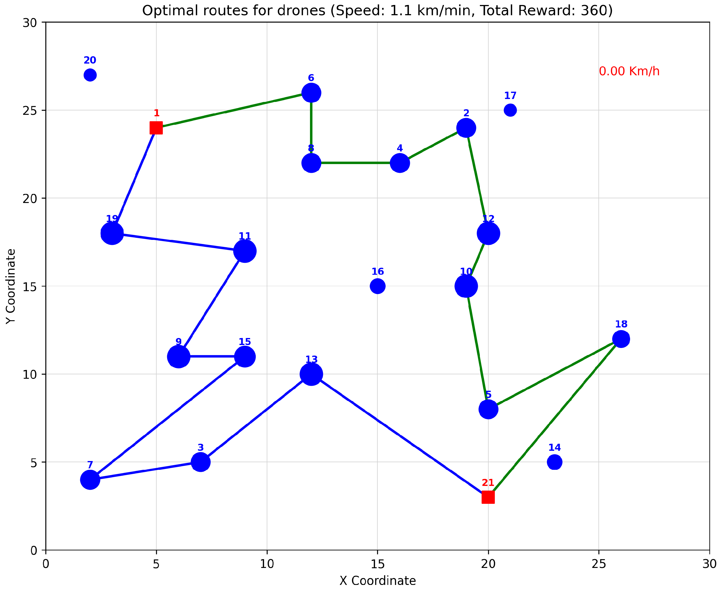
5.1. Solving the Standard TOP Without Obstacles or Environmental Factors

To establish a performance baseline, we solved the simple version of the problem (without obstacles or environmental factors) using Gurobi, a commercial optimization solver. Two different instance sets were considered: a 21-node instance with two UAVs and a 31-node instance with three UAVs. For the 21-node instance with two UAVs, each with a speed of $1.1$ km/min and a maximum route duration of 50 min, the solver identified an optimal solution with a total reward of $360.0$. Figure 9 illustrates the optimal routes identified by Gurobi.

The optimal routes for the UAVs are as follows: drone 1 route is [1, 8, 6, 2, 4, 12, 10, 18, 5, 21], with total distance $=50.81$ km, travel time = 46.19 min, and route reward = $175.0$; drone 2 route is [1, 19, 11, 9, 3, 7, 15, 13, 21], with total distance = $53.99$ km, travel time = $49.08$ min, and route reward = $185.0$.

For the more complex 31-node instance with three UAVs, each with a speed of $1.1$ km/min and a maximum route duration of 50 min, Gurobi found an optimal solution with a total reward of $543.0$. Figure 10 illustrates these optimal routes.

The optimal routes are as follows: drone 1 route is [1, 17, 10, 8, 4, 6, 7, 21, 30, 31], with total distance = 54.99 km, travel time = 49.99 min, and route reward = 163.0; drone 2 route is [1, 3, 25, 14, 23, 13, 11, 29, 5, 31] with total distance = 48.37 km, travel time = 43.97 min, and route reward = 170.0; drone 3 route is [1, 19, 27, 16, 20, 18, 9, 15, 12, 26, 2, 24, 28, 31], with total distance = 54.27 km, travel time = 49.34 min, and route reward = 210.0.

When applying our proposed A*-based neural network approach to the 21-node instance without obstacles, our algorithm achieved a solution with a total reward of $345.0$. The routes generated were as follows: route 1 = [1, 19, 9, 15, 13, 11, 16, 5, 21], with reward = 175.0, and travel time 45.81 min; route 2 = [1, 6, 8, 4, 2, 17, 12, 10, 18, 14, 21], with reward = 170.0, and travel time = 48.33 min.

For the more complex 31-node instance without obstacles, our algorithm achieved a total reward of $503.0$. The routes generated by our algorithm are: route 1 = [1, 3, 25, 14, 23, 13, 29, 11, 18, 9, 15, 12, 31], with reward = 238.0, and travel time = 49.93 min; route 2 = [1, 17, 7, 28, 30, 19, 21, 24, 31], with reward = 150.0, and travel time = 43.60 min; and route 3 = [1, 10, 8, 4, 6, 2, 26, 22, 31], with reward = 115.0, and travel time = 45.47 min.

5.2. Solving the TOP with Obstacles and Environmental Factors

In this section, we extend our analysis to evaluate the robustness of our approach under more realistic operational conditions. We examine how environmental factors such as obstacles, wind conditions, and payload weight affect route optimization in Scenario 1 (the one with 21 nodes).

We first analyze the effect of obstacles on route planning. Figure 11 illustrates the optimal routes generated by our algorithm for Scenario 1 with obstacles, UAV speed of $1.1$ km/min, payload of $1.0$ kg, and wind speed of $0.2$ km/min at 0° direction (easterly wind). The presence of obstacles (represented by black rectangles) significantly impacts the routes, forcing UAVs to take detours that increase travel times and distances. Our algorithm successfully generated feasible routes that avoid all obstacles while maximizing reward collection.

Our best solution (OBD) for this variant with obstacles is as follows: route 1 = [1, 11, 19, 9, 15, 13, 21], with reward = 145.0, and travel time = 49.54 min; and route 2 = [1, 8, 4, 2, 12, 10, 5, 21], with reward = 140.0, and travel time = 49.82 min. The total reward was $285.0$.

To investigate the impact of wind conditions on route optimization, we conducted experiments with constant drone speed ($1.1$ km/min), payload ($1.0$ kg), and wind speed ($0.2$ km/min) while varying the wind direction. This analysis reveals how our algorithm adapts routes based on prevailing wind conditions. As can be seen in Figure 12, with a northerly wind our algorithm generated more conservative routes: route 1 = [1, 19, 11, 13, 21], with reward 90.0, and travel time 48.88 min; and route 2 = [1, 8, 16, 5, 21], with reward = 50.0, and travel time 49.55 min. The total deterministic reward decreased to 140.0.

Several key observations emerge from this analysis: (i) wind direction substantially impacts achievable rewards due to the specific geographic distribution of nodes; (ii) the neural network demonstrates remarkable adaptability across different wind directions; and (iii) the algorithm maintains consistent computational performance across all wind directions, with average computation times ranging from $64.15$ to $64.63$ s per iteration.

We also examined the impact of travel time stochasticity on solution reliability. Using a constant variance level parameter $\lambda =0.3$, we conducted multiple simulation runs to evaluate how solutions optimized for deterministic conditions performed under uncertainty. This moderate level of variability typically resulted in simulation-based reward estimates (OBS) that were approximately 10–15% lower than their deterministic counterparts (OBD), highlighting the importance of accounting for uncertainty during the optimization process. The consistent gap between deterministic and stochastic solution quality demonstrates the value of our simheuristic approach, which explicitly accounts for uncertainty when evaluating and selecting solutions. Without this consideration, planners might overestimate the achievable rewards in real-world deployments, leading to suboptimal resource allocation and mission planning. The combined effect of obstacles, payload weight, and wind conditions creates a complex optimization scenario that traditional exact solvers would not be able to address efficiently. Our neural network-based approach demonstrates robust performance across these varying conditions, providing solutions that balance reward maximization with route feasibility and reliability.

6. Discussion and Conclusions

In this study, we developed a method for calculating the travel time of a UAV along a path defined by two nodes, considering the complexity of factors such as UAV speed, payload, wind conditions, and geometric aspects of the path. By treating this calculation as a ‘black box’ we have addressed the nonlinearity and interdependencies of these factors, which would otherwise make explicit modeling challenging.

To enhance computational efficiency and accuracy, we introduced a neural network model capable of estimating the time required to traverse individual path segments. This modular approach allows for real-time estimation across various trajectories, even in dynamic and complex environments. The network was trained using simulated data and validated with real-world conditions, demonstrating the system’s ability to learn complex patterns and generalize across new scenarios. The iterative training process further refined the model’s predictions, reducing discrepancies between estimated and real travel times.

Our model’s ability to account for travel time uncertainty through stochastic modeling represents a significant advancement in practical UAV route planning. By classifying edges based on destination node characteristics and employing lognormal distributions with a moderate variability level ($\lambda =0.3$) to model travel time uncertainty, we have created a framework that balances computational efficiency with realistic representation of operational uncertainties. The simulation results show that solutions optimized without considering uncertainty can significantly underperform when deployed in real-world conditions.

This study fills an important gap in the literature on the team orienteering problem in environments with physical obstacles and dynamic environmental factors, conditions that are rarely considered in traditional TOP research. By combining A* path-finding with neural network-based travel time prediction, our approach introduces a flexible, data-driven framework capable of handling complex routing scenarios in realistic UAV applications. The proposed methodology also has relevant implications for Robotic Engineering, particularly in the design of autonomous navigation and control systems. By integrating classical path planning (A*) with data-driven travel time prediction through neural networks, the approach supports more informed and adaptive navigation in dynamic and constrained environments. This hybrid model enables robots or UAVs to make route decisions based not only on geometry but also on external conditions such as wind or payload effects, which are often critical in real-world deployment.

Still, the proposed methodology has several practical limitations. Combining the A* algorithm with neural network predictions increases both memory usage and computational demands. The memory required by the A* algorithm can become excessive in large or detailed grid environments, while performance on a 30 × 30 km grid with moderate obstacles was acceptable, scaling to larger or denser environments would require further memory optimizations. Additionally, training the neural network demands significant processing power, especially in early iterations. Another limitation is the dependency of prediction accuracy on the volume and variety of training data. In the initial stages, with limited data, the model’s travel time estimates can be inaccurate, leading to less optimal routing.

Future work will focus on enhancing the model’s adaptability and accuracy by incorporating real-time data integration, such as live environmental factors, weather, and traffic conditions. This would improve the system’s ability to make dynamic adjustments during operation. Additionally, expanding the framework to accommodate multi-UAV collaboration could optimize route efficiency across several UAVs, considering communication and coordination constraints. This would allow the system to scale and handle more complex operational scenarios.

References

1. Chao, I.M.; Golden, B.L.; Wasil, E.A. The team orienteering problem. Eur. J. Oper. Res. 1996, 88, 464–474. [Google Scholar] [CrossRef]
2. Gunawan, A.; Lau, H.C.; Vansteenwegen, P. Orienteering Problem: A survey of recent variants, solution approaches and applications. Eur. J. Oper. Res. 2016, 255, 315–332. [Google Scholar] [CrossRef]
3. Xu, W.; Xu, Z.; Peng, J.; Liang, W.; Liu, T.; Jia, X.; Das, S.K. Approximation Algorithms for the Team Orienteering Problem. In Proceedings of the IEEE INFOCOM 2020-IEEE Conference on Computer Communications, Toronto, ON, Canada, 6–9 July 2020; pp. 1389–1398. [Google Scholar] [CrossRef]
4. Boussier, S.; Feillet, D.; Gendreau, M. An exact algorithm for team orienteering problems. 4OR 2007, 5, 211–230. [Google Scholar] [CrossRef]
5. Vansteenwegen, P.; Souffriau, W.; Oudheusden, D.V. The orienteering problem: A survey. Eur. J. Oper. Res. 2011, 209, 1–10. [Google Scholar] [CrossRef]
6. Panadero, J.; Juan, A.A.; Ghorbani, E.; Faulin, J.; Pagès-Bernaus, A. Solving the stochastic team orienteering problem: Comparing simheuristics with the sample average approximation method. Int. Trans. Oper. Res. 2024, 31, 3036–3060. [Google Scholar] [CrossRef]
7. Vansteenwegen, P.; Gunawan, A. Orienteering Problems; Springer: Cham, Switzerland, 2019. [Google Scholar]
8. Aringhieri, R.; Bigharaz, S.; Duma, D.; Guastalla, A. Novel Applications of the Team Orienteering Problem in Health Care Logistics. In Proceedings of the Optimization in Artificial Intelligence and Data Sciences; Amorosi, L., Dell’Olmo, P., Lari, I., Eds.; Springer: Cham, Switzerland, 2022; pp. 235–245. [Google Scholar] [CrossRef]
9. Moosavi Heris, F.S.; Ghannadpour, S.F.; Bagheri, M.; Zandieh, F. A new accessibility based team orienteering approach for urban tourism routes optimization (A Real Life Case). Comput. Oper. Res. 2022, 138, 105620. [Google Scholar] [CrossRef]
10. Du, J.; Wu, P. Deep reinforcement learning for UAVs rolling horizon team orienteering problem under ECA. Ocean Eng. 2025, 326, 120781. [Google Scholar] [CrossRef]
11. Foead, D.; Ghifari, A.; Kusuma, M.B.; Hanafiah, N.; Gunawan, E. A systematic literature review of A* pathfinding. Procedia Comput. Sci. 2021, 179, 507–514. [Google Scholar] [CrossRef]
12. Farid, G.; Cocuzza, S.; Younas, T.; Razzaqi, A.A.; Wattoo, W.A.; Cannella, F.; Mo, H. Modified A-Star (A*) Approach to Plan the Motion of a Quadrotor UAV in Three-Dimensional Obstacle-Cluttered Environment. Appl. Sci. 2022, 12, 5791. [Google Scholar] [CrossRef]
13. Nehra, N.; Sangwan, P.; Kumar, D. Artificial neural networks: A comprehensive review. In Handbook of Machine Learning for Computational Optimization; Taylor Francis: Boca Raton, FL, USA, 2021; pp. 203–227. [Google Scholar]
14. Kirac, E.; Milburn, A.B.; Gedik, R. The Dynamic Team Orienteering Problem. Eur. J. Oper. Res. 2025, 324, 22–39. [Google Scholar] [CrossRef]
15. Vansteenwegen, P.; Souffriau, W.; Berghe, G.V.; Van Oudheusden, D. Iterated local search for the team orienteering problem with time windows. Comput. Oper. Res. 2009, 36, 3281–3290. [Google Scholar] [CrossRef]
16. Gunawan, A.; Ng, K.M.; Kendall, G.; Lai, J. An iterated local search algorithm for the team orienteering problem with variable profits. Eng. Optim. 2018, 50, 1148–1163. [Google Scholar] [CrossRef]
17. Vincent, F.Y.; Salsabila, N.Y.; Lin, S.W.; Gunawan, A. Simulated annealing with reinforcement learning for the set team orienteering problem with time windows. Expert Syst. Appl. 2024, 238, 121996. [Google Scholar]
18. Lin, S.W.; Vincent, F.Y. A simulated annealing heuristic for the team orienteering problem with time windows. Eur. J. Oper. Res. 2012, 217, 94–107. [Google Scholar] [CrossRef]
19. Narin, A.B.; Becker, J.; Batta, R. UAV search optimization for recording emerging targets with camouflaging capabilities. J. Def. Model. Simul. 2023, 22, 15485129231203020. [Google Scholar] [CrossRef]
20. Fang, C.; Han, Z.; Wang, W.; Zio, E. Routing UAVs in landslides Monitoring: A neural network heuristic for team orienteering with mandatory visits. Transp. Res. Part E Logist. Transp. Rev. 2023, 175, 103172. [Google Scholar] [CrossRef]
21. Zhu, M.; Du, X.; Zhang, X.; Luo, H.; Wang, G. Multi-UAV rapid-assessment task-assignment problem in a post-earthquake scenario. IEEE Access 2019, 7, 74542–74557. [Google Scholar] [CrossRef]
22. Li, Y.; Peyman, M.; Panadero, J.; Juan, A.A.; Xhafa, F. IoT analytics and agile optimization for solving dynamic team orienteering problems with mandatory visits. Mathematics 2022, 10, 982. [Google Scholar] [CrossRef]
23. Bayliss, C.; Juan, A.A.; Currie, C.S.; Panadero, J. A learnheuristic approach for the team orienteering problem with aerial drone motion constraints. Appl. Soft Comput. 2020, 92, 106280. [Google Scholar] [CrossRef]
24. Hussein, A.A.; Yaseen, E.T.; Rashid, A.N. Learnheuristics in routing and scheduling problems: A review. Samarra J. Pure Appl. Sci. 2023, 5, 60–90. [Google Scholar] [CrossRef]
25. Uguina, A.R.; Gomez, J.F.; Panadero, J.; Martínez-Gavara, A.; Juan, A.A. A Learnheuristic Algorithm Based on Thompson Sampling for the Heterogeneous and Dynamic Team Orienteering Problem. Mathematics 2024, 12, 1758. [Google Scholar] [CrossRef]
26. Nekovář, F.; Faigl, J.; Saska, M. Multi-vehicle dynamic water surface monitoring. IEEE Robot. Autom. Lett. 2023, 8, 6323–6330. [Google Scholar] [CrossRef]
27. Zhu, M.; Zhang, X.; Luo, H.; Wang, G.; Zhang, B. Optimization Dubins path of multiple UAVs for post-earthquake rapid-assessment. Appl. Sci. 2020, 10, 1388. [Google Scholar] [CrossRef]
Figure 1. Example of trajectories with UAVs avoiding obstacles on a 30 × 30 km grid.
Algorithms 18 00309 g001
Figure 2. Example of a TOP solution with UAVs avoiding obstacles on a 30 × 30 km grid.
Algorithms 18 00309 g002
Figure 3. General overview of our approach.
Algorithms 18 00309 g003
Figure 4. A schema of Stage 1.
Algorithms 18 00309 g004
Figure 5. A schema of Stage 2.
Algorithms 18 00309 g005
Figure 6. Interaction between the A* and the neural network predictor.
Algorithms 18 00309 g006
Figure 7. Architecture of the proposed neural network.
Algorithms 18 00309 g007
Figure 8. Base instances with and without obstacles.
Algorithms 18 00309 g008
Figure 9. Optimal routes for the 21-node instance without obstacles.
Algorithms 18 00309 g009
Figure 10. Optimal routes for the 31-node instance without obstacles.
Algorithms 18 00309 g010
Figure 11. Route optimization under obstacle constraints.
Algorithms 18 00309 g011
Figure 12. Route optimization under northerly wind conditions.
Algorithms 18 00309 g012
Disclaimer/Publisher’s Note: The statements, opinions and data contained in all publications are solely those of the individual author(s) and contributor(s) and not of MDPI and/or the editor(s). MDPI and/or the editor(s) disclaim responsibility for any injury to people or property resulting from any ideas, methods, instructions or products referred to in the content.