Patient-Specific Hyperparameter Optimization of a Deep Learning-Based Tumor Autocontouring Algorithm on 2D Liver, Prostate, and Lung Cine MR Images: A Pilot Study

Abstract

Linear accelerator–magnetic resonance (linac-MR) hybrid systems allow for real-time magnetic resonance imaging (MRI)-guided radiotherapy for more accurate dose delivery to the tumor and improved sparing of the adjacent healthy tissues. However, for real-time tumor detection, it is unfeasible for a human expert to manually contour (gold standard) the tumor at the fast imaging rate of a linac-MR. This study aims to develop a neural network-based tumor autocontouring algorithm with patient-specific hyperparameter optimization (HPO) and to validate its contouring accuracy using in vivo MR images of cancer patients. Two-dimensional (2D) intrafractional MR images were acquired at 4 frames/s using 3 tesla (T) MRI from 11 liver, 24 prostate, and 12 lung cancer patients. A U-Net architecture was applied for tumor autocontouring and was further enhanced by implementing HPO using the Covariance Matrix Adaptation Evolution Strategy. Six hyperparameters were optimized for each patient, for which intrafractional images and experts’ manual contours were input into the algorithm to find the optimal set of hyperparameters. For evaluation, Dice’s coefficient (DC), centroid displacement (CD), and Hausdorff distance (HD) were computed between the manual contours and autocontours. The performance of the algorithm was benchmarked against two standardized autosegmentation methods: non-optimized U-Net and nnU-Net. For the proposed algorithm, the mean (standard deviation) DC, CD, and HD of the 47 patients were 0.92 (0.04), 1.35 (1.03), and 3.63 (2.17) mm, respectively. Compared to the two benchmarking autosegmentation methods, the proposed algorithm achieved the best overall performance in terms of contouring accuracy and speed. This work presents the first tumor autocontouring algorithm applicable to the intrafractional MR images of liver and prostate cancer patients for real-time tumor-tracked radiotherapy. The proposed algorithm performs patient-specific HPO, enabling accurate tumor delineation comparable to that of experts.

1. Introduction

During radiation therapy, intrafractional tumor motion poses a significant challenge in accurately irradiating the tumor and minimizing healthy tissue irradiation. This becomes more challenging when the tumor has a large range of motion and undergoes shape deformation due to respiratory and cardiac activities (e.g., lung and liver tumors) [1,2,3]. To minimize healthy tissue irradiation while treating mobile tumors, intrafractional tumor tracking (i.e., following the tumor with a treatment beam) has been widely studied in the past. For target monitoring (i.e., estimating the target position as a function of time) in intrafractional tumor tracking, various approaches have been proposed, which can be categorized into two types: non-invasive and invasive. One non-invasive approach is infrared-based monitoring (e.g., Varian Real-time Position Management (RPM) system); during treatment, the location of an external marker block placed on the patient’s surface is monitored by an infrared camera system [4,5]. This information is used to estimate the internal tumor position based on the correlation between the location of the marker block and the tumor centroid, where the correlation is established prior to the treatment using planning computed tomography (CT) images [4]. Another non-invasive approach is optical surface monitoring (e.g., AlignRT system), which uses multiple high-definition cameras to project structured light patterns on the patient such that motion can be estimated [5,6]. During treatment, the real-time detected patient surface is compared with a reference surface, often obtained from the simulation CT [6], and this information is used to estimate the tumor position based on the correlation between the alignment of the patient and the alignment of the tumor determined by an additional system [5]. Invasive approaches include X-ray image-based methods, which come in different hardware configurations of stereoscopic imaging and can be combined with external monitoring [6]. The CyberKnife system uses both external and internal tumor surrogates to estimate tumor positions during beam delivery. The patient wears a vest containing external markers that are monitored by a camera system to update the patient’s external motion. Metallic surrogates are also surgically inserted near the tumor and are imaged by two orthogonal kilovoltage X-ray systems. During treatment, the tumor position is estimated by the assumed correlation between the patient’s external motion and the location of internal surrogates, where the correlation is established prior to the treatment and periodically updated using the X-ray images. Real-time tumor tracking radiotherapy (RTRT) and Vero systems use metallic seeds as internal tumor surrogates, which are monitored during treatment by two orthogonal diagnostic X-ray systems in fluoroscopic mode. These images are used to estimate the internal tumor’s position [6]. With information from target monitoring, various tracking methods can be used for beam delivery, which include robotic tracking through CyberKnife Synchrony [7], gimbaled tracking through BrainLab Vero [8,9], couch tracking [10], and multi-leaf collimator (MLC) tracking [11,12]. These methods have the potential for margin reduction, particularly for targets affected by respiratory motion where the internal target volume (ITV) is reduced [13].

Most of the currently available target monitoring methods are based on indirect tracking through the use of internal or external tumor surrogates [6]. Reliance on surrogates, however, has been shown to be problematic because implanted seeds can migrate from their initial positions [14], good correlations between internal tumor motion and external surrogate displacement are assumed while mismatches between tumor and surrogates have been shown [15,16], and any tumor shape deformation is unknown during tracking. A hybrid radiotherapy–magnetic resonance (MR) system known as linac-MR [17,18,19,20] overcomes these limitations by enabling intrafractional MR imaging of a tumor.

By providing intrafractional MR images of tumor regions with sufficient soft tissue contrast concurrently with irradiation, linac-MR has the potential to achieve non-invasive intrafractional tumor-tracked radiotherapy (nifteRT). During nifteRT, the treatment beam can follow the mobile tumor based on the intrafractional MR images, by adaptively adjusting its shape and position via MLC control. The feasibility of nifteRT using linac-MR was demonstrated by Yun et al. [21] through tracking and irradiating a phantom undergoing simulated tumor motions. Similarly, other feasibility studies have shown the possibility of magnetic resonance imaging (MRI)-guided tumor tracking for improving tumor localization and sparing of healthy tissues [22,23].

For nifteRT using linac-MR, the first step is to detect the shape and position of the tumor in each MR image. Currently, common clinical practice requires a certified expert (e.g., radiation oncologist) to manually detect and contour the tumor and the organs during the MR simulation session performed prior to treatment. However, it is not feasible for a human expert to continually contour images at the fast imaging rate of linac-MR (>4 frames/s) for the duration of treatment. To address this, a previous study by Yun et al. [24] developed an artificial neural network-based autocontouring algorithm (pulse-coupled neural network), which achieved ~90% contouring accuracy compared to experts’ manual contours for lung cancer patients. However, this was not achieved for other sites such as the liver and prostate. For both of these sites, autocontouring becomes challenging as both the low image contrast and unclear boundary between the tumor and tissue background make it difficult for the algorithm to learn details of the tumor’s shape.

The aim of this pilot study is to address this issue by employing (1) a deep neural network and (2) hyperparameter optimization (HPO) powered by the Covariance Matrix Adaptation Evolution Strategy (CMA-ES) [25], in our autocontouring algorithm. Semantic image segmentation, which refers to the process of transforming raw medical images into clinically relevant, spatially structured information, such as outlining tumor boundaries, is the most widely investigated medical image processing task, with numerous segmentation algorithms published in the field of biomedical image segmentation each year [26,27]. One of the first deep learning-based segmentation algorithms was a fully convolutional network (FCN) [28], which includes only convolutional layers that enable it to take an image of arbitrary size and generate a segmentation map of the same size [29]. However, by following the design principle of classification networks, global context information is not taken into account in an efficient way, potentially ignoring useful scene-level context [29,30]. Ronneberger et al. [31] proposed U-Net, which is built upon an FCN for medical image segmentation. U-Net uses concatenations in a symmetric network architecture to combine global context information from shallower layers and semantic information from deeper layers to improve segmentation details. For tumor segmentation, U-Net-based architectures are extensively used and modified to improve segmentation performance [32,33]. As there now exist numerous segmentation algorithms, various public challenges and benchmarks have been organized in the past for lung, liver, and prostate tumor segmentation to serve as the standard for comparative assessment of segmentation algorithms [26,32,33].

In order for a segmentation algorithm to achieve optimal performance for a given task, it is essential to properly tune the hyperparameters that determine its network architecture and control the training process. Some commonly used HPO methods include grid search, random search, and Bayesian optimization [34]. Since grid search and random search have no means of directing the search towards better solutions, they may not lead to the best solutions and require a long execution time. Bayesian optimization is known to perform well for optimizing continuous hyperparameters. However, it is sequential by nature, and thus, it is often too slow for practical use in large-scale neural networks and is more suitable for small function evaluation budgets (i.e., the number of iterations searching for optimal hyperparameters may be limited due to excessive computing time; for example, <10 times the number of hyperparameters being optimized) [34,35]. CMA-ES is considered as a state-of-the-art optimizer for continuous black-box functions, which may prevent premature convergence and lead to fast convergence by step size control and covariance matrix adaptation, as well as support parallel evaluations of solutions [34]. Loshchilov et al. [36] showed that CMA-ES performed best among more than 100 classic and modern optimizers for various black-box functions with moderate to large evaluation budgets. Compared to various state-of-the-art Bayesian optimization methods such as Tree Parzen Estimator (TPE) and Sequential Model-Based Algorithm Configuration (SMAC), CMA-ES can be more powerful, especially in the regime of parallel evaluations [34]. In a study by Wollmann et al. [37], optimizing three hyperparameters using CMA-ES showed superior performance over TPE and SMAC for segmenting cell nuclei in prostate tissue images.

In this work, HPO with CMA-ES has been implemented to improve the contouring accuracy of a U-Net-based autocontouring algorithm for challenging anatomic sites. For each patient, our algorithm generates patient-specific hyperparameters and trainable parameters using the same patient’s cine MR images. Patient-specific HPO was chosen because, in clinical practice, a single physician is typically responsible for a patient’s treatment, and each physician defines target volumes based on their individual experience and clinical judgment. In nifteRT, our aim is to precisely replicate a specific physician’s contouring style for each patient, rather than generating generalized or consensus-based contours. This level of personalization is likely essential for clinical acceptance of the real-time autocontouring feature in nifteRT. In clinic, the patient’s cine MR images are to be acquired during the MR simulation session prior to the actual treatment using the same imaging sequence and patient setup as in the treatment. The contouring performance of the algorithm for various liver, prostate, and lung cancer patients is presented and compared to that of the standardized segmentation methods. The main contributions of our work are the following:

• Patient-specific HPO was performed, tailoring the hyperparameters for each patient dataset to achieve the best possible autocontouring performance.
• The first application of CMA-ES for optimizing the hyperparameters of a U-Net-based autocontouring algorithm is presented.
• The proposed algorithm is the first tumor autocontouring algorithm specifically applicable to the intrafractional MR images of liver and prostate cancer patients for nifteRT.
• The proposed algorithm achieved the best overall performance among standardized segmentation algorithms such as U-Net [31] and nnU-Net [27].
• A total of 47 in vivo MR image sets were acquired to evaluate the algorithm, which achieved comparable contouring performance to that of human experts.

2. Materials and Methods

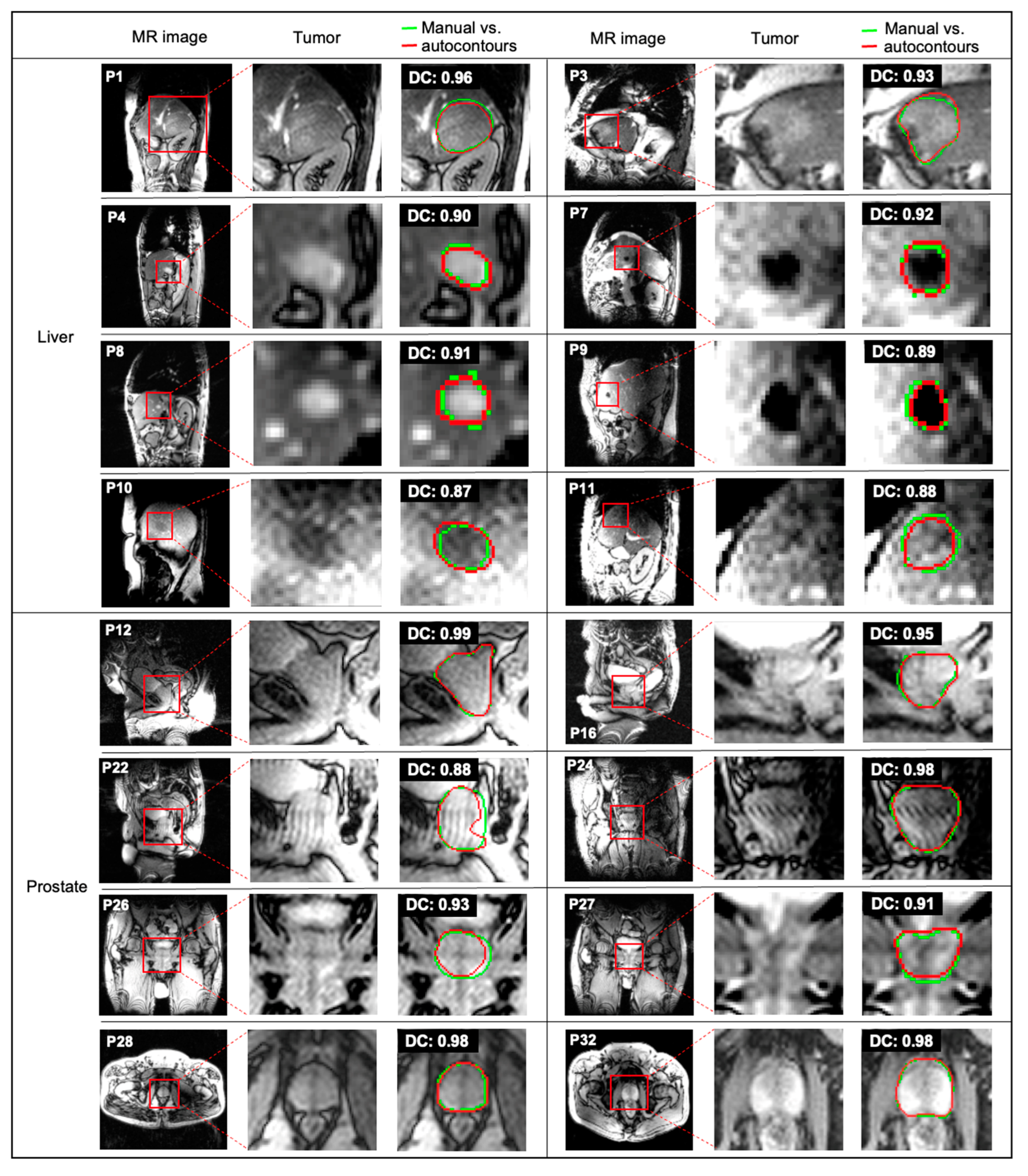
2.1. Patient Imaging and Manual Contouring

In this study, 11 liver, 24 prostate, and 12 lung cancer patients (see

Table 1. Characteristics of the liver, prostate (sagittal: P12–22, coronal: P23–27, axial: P28–35), and lung cancer patients included in this study. F: female; M: male; HCC: hepatocellular carcinoma; NSCLC: non-small-cell lung cancer; SCLC: small-cell lung cancer; SD: standard deviation.

Site	Patient	Gender	Age	Tumor Area (cm2)	Overall Stage	Cancer Type
Liver	1	F	65	36.2	III	Rectal adenocarcinoma
	2	M	69	11.5	I	HCC
	3	M	70	24.2	IV	Sigmoid colon adenocarcinoma
	4	M	57	2.8	I	HCC
	5	M	64	2.0	II	HCC
	6	M	63	3.7	IVB	Nasopharyngeal carcinoma
	7	M	65	3.1	IVA	Colorectal carcinoma
	8	M	59	2.4	IV	Adenocarcinoma
	9	M	68	1.5	IIB	Rectal adenocarcinoma
	10	F	82	6.0	IV	Colorectal cancer
	11	M	71	6.2	I	HCC
Prostate	12	M	66	23.3	IIA	Prostatic adenocarcinoma
	13	M	71	14.0	IIIB	Prostatic adenocarcinoma
	14	M	75	21.8	IIB	Prostatic adenocarcinoma
	15	M	62	12.2	IIIB	Prostatic adenocarcinoma
	16	M	66	15.9	I	Prostatic adenocarcinoma
	17	M	76	13.7	I	Prostatic adenocarcinoma
	18	M	77	24.5	IIC	Prostatic adenocarcinoma
	19	M	70	18.7	IIB	Prostatic adenocarcinoma
	20	M	69	8.4	IIIC	Prostatic adenocarcinoma
	21	M	63	4.7	IIB	Prostatic adenocarcinoma
	22	M	66	22.2	IIC	Prostatic adenocarcinoma
	23	M	70	20.1	IIB	Prostatic adenocarcinoma
	24	M	66	22.8	IIC	Prostatic adenocarcinoma
	25	M	77	26.9	IIC	Prostatic adenocarcinoma
	26	M	69	13.3	IIIC	Prostatic adenocarcinoma
	27	M	63	9.2	IIB	Prostatic adenocarcinoma
	28	M	62	11.6	IIIB	Prostatic adenocarcinoma
	29	M	69	13.9	IIIC	Prostatic adenocarcinoma
	30	M	66	19.7	IIC	Prostatic adenocarcinoma
	31	M	66	13.1	I	Prostatic adenocarcinoma
	32	M	75	26.4	IIB	Prostatic adenocarcinoma
	33	M	63	12.7	IIB	Prostatic adenocarcinoma
	34	M	70	14.3	IIB	Prostatic adenocarcinoma
	35	M	77	17.7	IIC	Prostatic adenocarcinoma
Lung	36	F	73	6.4	II	NSCLC
	37	M	65	3.8	IA	NSCLC
	38	F	78	7.4	I	Lung cancer
	39	M	79	3.8	I	NSCLC
	40	M	65	5.1	I	NSCLC
	41	M	90	3.9	I	Squamous cell carcinoma
	42	M	75	3.7	I	NSCLC
	43	M	81	1.3	I	NSCLC
	44	M	75	3.0	IIA	NSCLC
	45	M	70	1.7	IB	SCLC
	46	M	65	1.4	IA	NSCLC
	47	M	72	4.8	IVA	NSCLC
Mean (SD)				11.6 (8.7)

for patient characteristics) were scanned between 28 September 2011 and 15 June 2022 using a 3 tesla (T) MRI (Philips Achieva, Eindhoven, the Netherlands) with a balanced steady-state free precession (bSSFP) sequence (field of view = 30 × 40 to 40 × 40 cm², acquisition matrix size = 128 × 128, reconstructed matrix size = 256 × 256, voxel size = 2.3 × 3.1 × 10–3.1 × 3.1 × 15 mm³, echo time = 1.1 ms, repetition time = 2.2 ms, imaging time per frame = 275 ms) to acquire > 300 dynamic images per patient (approximately 2 min imaging time). The patients did not receive motion management nor breathing guidance during the scan. For liver and lung patients, the sagittal plane was imaged as it includes the superior–inferior direction, which is the dominant direction of liver and lung motion [38,39,40]. Each prostate patient was imaged in one of the three imaging planes (sagittal, coronal, and axial) as the dominant prostate motion is often not in one direction [41,42]. The same imaging plane was used throughout the training and testing of the algorithm for each patient. For these patients, our foremost clinical goal in nifteRT is to realize hypofractionated 3D conformal radiotherapy using linac-MR technology. Hypofractionation would be possible because treatment margin can be reduced via nifteRT without increasing the normal tissue complication probability. In nifteRT, we aim to remove or minimize the ITV margin, which is assigned to address intrafractional physiological movements and variations in size, shape, and position during irradiation. The planning target volume (PTV) margin accounting for the interfractional variations in anatomy and patient setup error will still be assigned as in the current treatment techniques.

For each patient, an expert (radiation oncologist) manually contoured the gross tumor volume in 130 consecutive images using either Computational Environment for Radiotherapy Research (CERR) [43] or 3D Slicer (version 4.11) [44] software. In this study, 130 images/patient was chosen to balance the burden of manual contouring and obtaining a sufficient number of testing images. This dataset was used to train the algorithm, as well as to serve as a reference for comparison to autocontours by dividing into 30 training, 30 validation, and 70 testing images. Only the training images were used to learn the trainable parameters (i.e., neural network weights) of the U-Net-based algorithm. The validation images were used to (1) monitor the prediction accuracy of a given model built by the current set of hyperparameters and to (2) apply early stopping (details in Section 2.3) to prevent overfitting. The testing images were unseen by the algorithm during HPO and training and were only used to evaluate the accuracy of the final, hyperparameter (HP)-optimized network [35]. The 30-30-70 ratio was empirically chosen to include at least two respiratory cycles in the training images and to use the same number of validation images as training images.

Regarding the data size, 47 patients were considered to be reasonable for this pilot study because our aim is to demonstrate patient-specific HPO and training of the algorithm to autocontour tumors that are unique to each patient. As tumors exhibit unique features for different patients, patient-specific models may perform better than a single general model that is trained on a large number of patients [45,46]. Recent studies aimed at building patient-specific models have also used a data size comparable to that used in this study (17 patients in Fransson et al. [47], 10 patients in Smolders et al. [45], and 36 patients in Jansen et al. [46]). In addition, there were practical limitations. Manual contouring of 130 images per patient, totaling 6110 images, imposed a significant workload for the radiation oncology experts involved. Also, recruiting a larger cohort of patients presented challenges in a clinical setting. Recruitment efforts are ongoing, with more patients being enlisted for future studies.

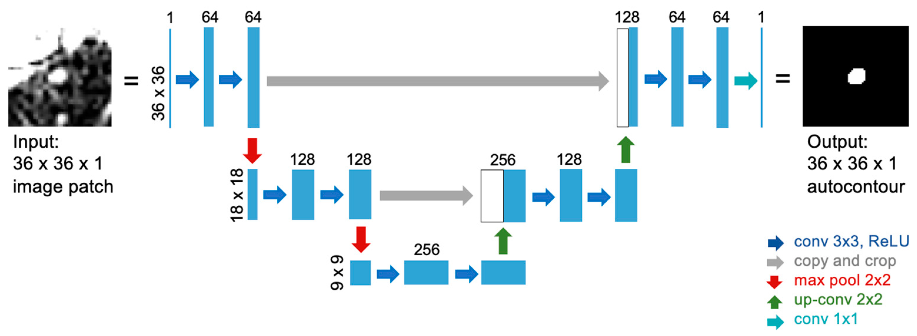
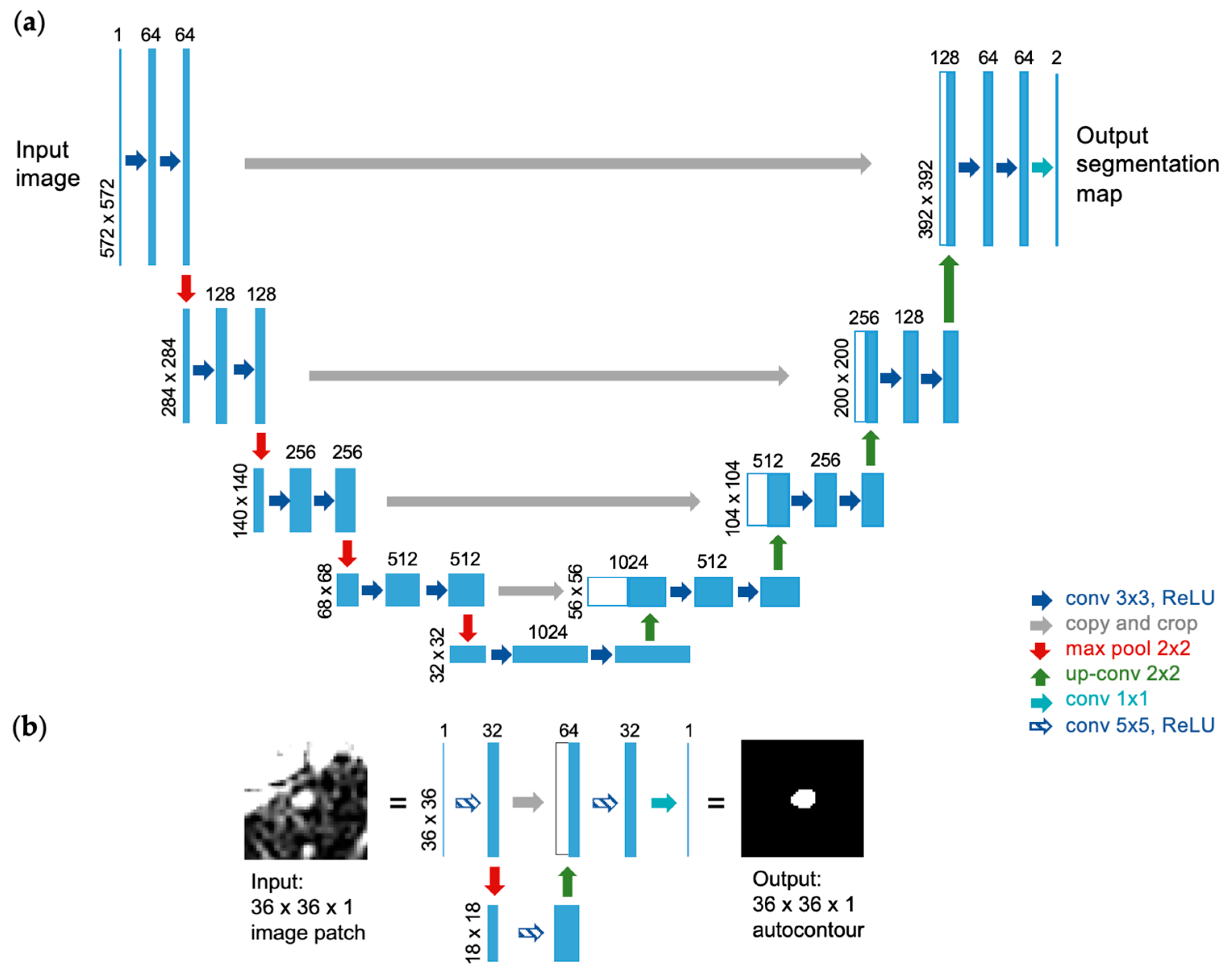
2.2. U-Net Implementation for Autocontouring Algorithm

Our overall aim was to achieve ≥0.9 contouring accuracy from the testing images, measured by Dice’s coefficient (DC; ∊[0, 1], where 1 means complete agreement) [48] between manual contours and autocontours. Since the mean (standard deviation (SD)) of intra- and interobserver variations in experts’ manual contouring were previously found as 0.88 (0.04) and 0.87 (0.04), respectively [49], which represent inherent uncertainties in manual contours, a comparable number of 0.9 was set as a goal to determine reasonable autocontouring accuracy.

As the first part of developing such an autocontouring algorithm, a deep neural network using a U-Net architecture was implemented. U-Net, initially developed for biomedical image segmentation by Ronneberger et al. [31], has been widely applied for segmentation tasks in medical imaging involving various sites, patients, and imaging modalities, for which it showed promising performance [50,51,52,53,54]. As opposed to classification tasks that require a label as output [55,56], segmentation tasks require a binary image as output; this makes U-Net a suitable choice due to its ability to localize the extracted features which allows to produce an accurate segmentation map as output. Also, U-Net can learn with a limited amount of training data, and it is faster to train than most other segmentation models due to its use of context-based learning [31,57].

U-Net is a convolutional neural network whose architecture consists of a contracting path for capturing context and a symmetric expanding path that enables precise localization (see Figure 4a, which is located under Section 3 for comparison to our modified version of U-Net). The contracting (or down-sampling) part extracts features with 3 × 3 convolutions, and the expanding (or up-sampling) part uses up-convolution, decreasing the number of feature maps while increasing their dimensions. A feature map is a collection of extracted features forming a 2D matrix that results from convolving an input image with a filter. For example, a 256 × 256 × 1 input image convolved with n number of 3 × 3 filters results in a 256 × 256 × n block of feature maps (using zero paddings to the input image to maintain the height and width dimensions after convolution), forming a 3D matrix. Feature maps from the expanding part are concatenated with the corresponding feature maps from the contracting part to recover localization information. Finally, a 1 × 1 convolution creates a linear projection of the feature maps to generate a binary segmentation map. For each patient case used in this study, the original U-Net architecture was modified by optimizing its hyperparameters.

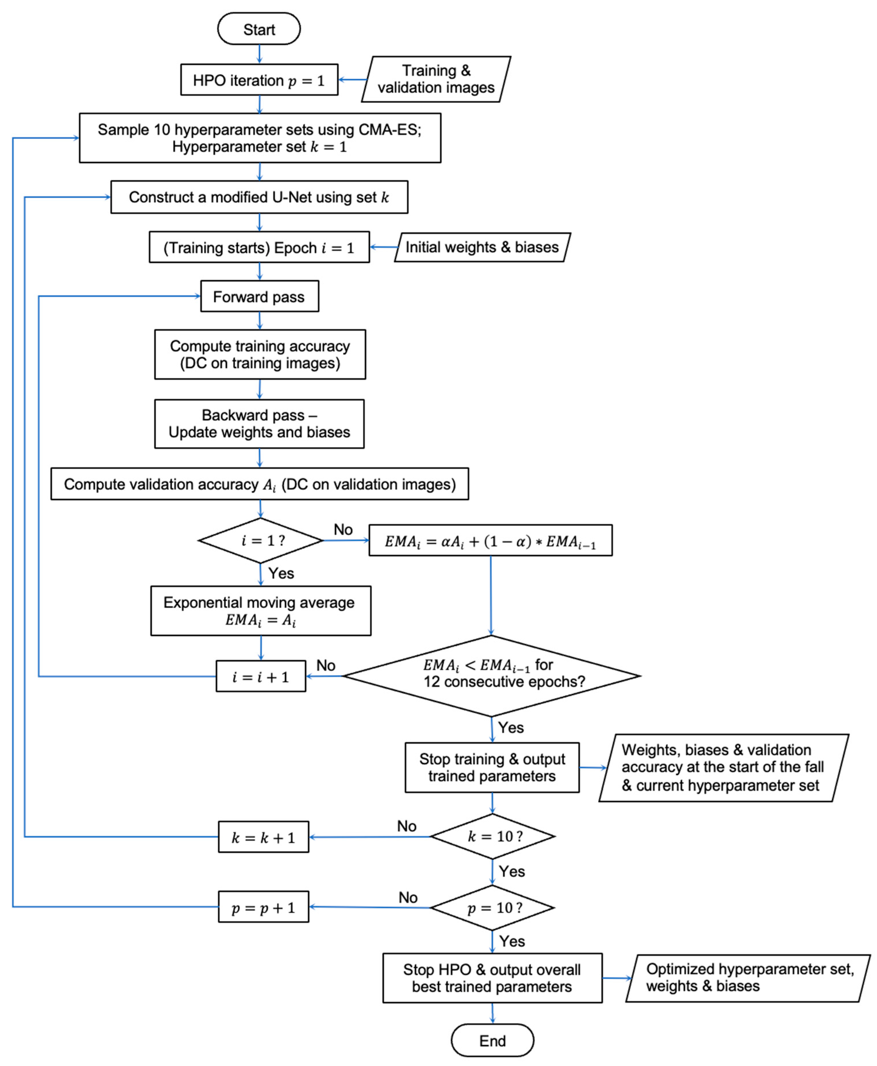
2.3. CMA-ES Implementation for HPO

The contouring performance of U-Net for a given task crucially depends on a wide range of hyperparameter choices [58]. Also, U-Net modified by HPO can be less computationally demanding than the original U-Net. As previously mentioned in Section 1, CMA-ES has advantages over other HPO methods by supporting parallel evaluations of solutions, potentially avoiding premature convergence and leading to fast convergence. Hence, HPO with CMA-ES was implemented to further develop the autocontouring algorithm. CMA-ES is a stochastic, population-based optimization algorithm for real-parameter optimization of non-linear, non-convex functions. It starts by creating a population of solutions randomly drawn from a normal distribution. By evaluating the objective function of each solution, the best portion of the population is selected, and the corresponding covariance matrix is calculated to adjust the shape of the next sampling distribution. This allows the search to move in the directions of the previously successful steps and may quickly converge to the global minimum.

The set of six hyperparameters—number of consecutive convolutions before or after each pooling or up-convolution, filter size for convolutions, number of feature maps, number of poolings, initial learning rate of the Adam optimizer, and number of training images—was independently optimized for each patient case within specified search ranges. The first four hyperparameters affecting the network size and the learning rate were chosen to be optimized as they often have a larger impact on the network performance [59]. The number of training images was also optimized as a hyperparameter, since it is a parameter outside the trainable parameters and is used to control the model performance [60,61]. Although optimizing a greater number of hyperparameters may improve the network performance, six hyperparameters were optimized in this work, which were empirically chosen to balance the network performance and computing time. Each of these hyperparameters with its search range in parentheses is described as follows:

• Number of consecutive convolutions (1 or 2): As a convolution operation extracts features from the input image, using multiple, consecutive convolutions allows us to extract more complex features that are combinations of simpler features that were previously extracted. As we have a small number of training images (30), a maximum of two convolutions was used to avoid creating too many weight parameters and thereby avoid overfitting.
• Filter size (3 or 5): A smaller filter (e.g., 3 $\times$ 3 matrix) extracts a larger amount of smaller and local features for a given input image, while a larger filter (e.g., 9 $\times$ 9 matrix) extracts a smaller amount of larger and broad features. A maximum of size 5 was used since a larger size may lead to overfitting, and an odd number was used for computational efficiency.
• Number of feature maps ([32, 128]): This refers to the number of filters applied to the input image during convolution. Despite 64 feature maps being used in the original U-Net [31], half of that number was used as the minimum as too small a number may not be sufficient to capture various shapes, and twice that number was used as the maximum as too large a number may cause overfitting.
• Number of poolings (1 or 2): A pooling operation down-samples the input image, reducing the sensitivity of the network to the location of features in the image. As each pooling is followed by convolutions in U-Net, the number of poolings largely affects the number of weight parameters to be used and thus the complexity of the network architecture. A maximum of two poolings was used since small image patches (e.g., 36 $\times$ 36) were used as input.
• Initial learning rate ([10⁻⁵, 10⁻¹]): This decides the initial step size the optimizer uses in the search space of weight parameters. With 10⁻³ being the default value used in the Adam optimizer [62], a range around this value was used since too large a number might cause the network to oscillate in the search space, while too low a number might take too long an execution time.
• Number of training images ([10, 30]): This refers to the number of annotated image pairs used to train the network. The maximum number of training images was set to 30 as it includes approximately two respiratory cycles, which were considered sufficient for the network to learn any respiration-induced tumor motion. Since using a smaller number of training images reduces the amount of labor for manual contouring, 10 was set as the minimum to test whether satisfactory performance can be achieved.

The overall HPO and training process is shown in Figure 1, which was executed for each patient case for patient-specific HPO. Starting with the first HPO iteration, 10 hyperparameter sets (solutions) were sampled using CMA-ES. The size of solution population for CMA-ES was maintained at 10 for faster execution time for all patient cases. Each solution was used to construct a modified U-Net, which was subsequently trained. The number of epochs for the training process of each solution was determined by an early stopping method. This method was implemented to prevent our networks from overfitting to the training images, rather than generalizing to all imaging data (training, validation, and testing images). The early stopping point (optimal number of epochs) was found for each solution by monitoring the exponential moving average (EMA) of validation accuracy, defined as follows:

$${EMA}_i=\left\{\begin{array}{c}{A}_i, i=1\hfill \\ \alpha A_i+\left(1-\alpha \right)\ast {EMA}_{i-1}, i>1\hfill \end{array}\right.$$

(1)

where $A_i$ is the validation accuracy (measured by DC on validation images) at epoch $i$, and $\alpha$ is the smoothing factor between 0 and 1. When the current EMA was less than the previous EMA for 12 consecutive epochs, which is an empirically determined number indicating no further improvement, training was stopped, and the weights and biases at the start of this fall were saved. A demonstrative sample result of the training accuracy and EMA of validation accuracy over epoch number for patient #9 (P9) is shown in Figure A1 in Appendix A. HPO was terminated after 10 iterations for the entire solution population, which resulted in a validation accuracy of ~0.9 for all patient cases.

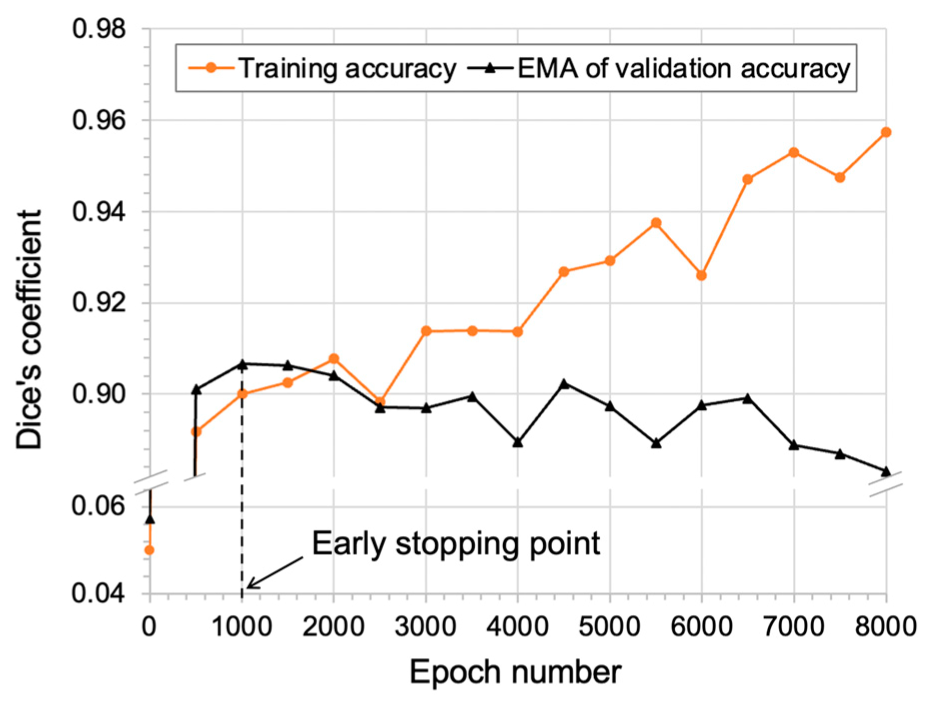
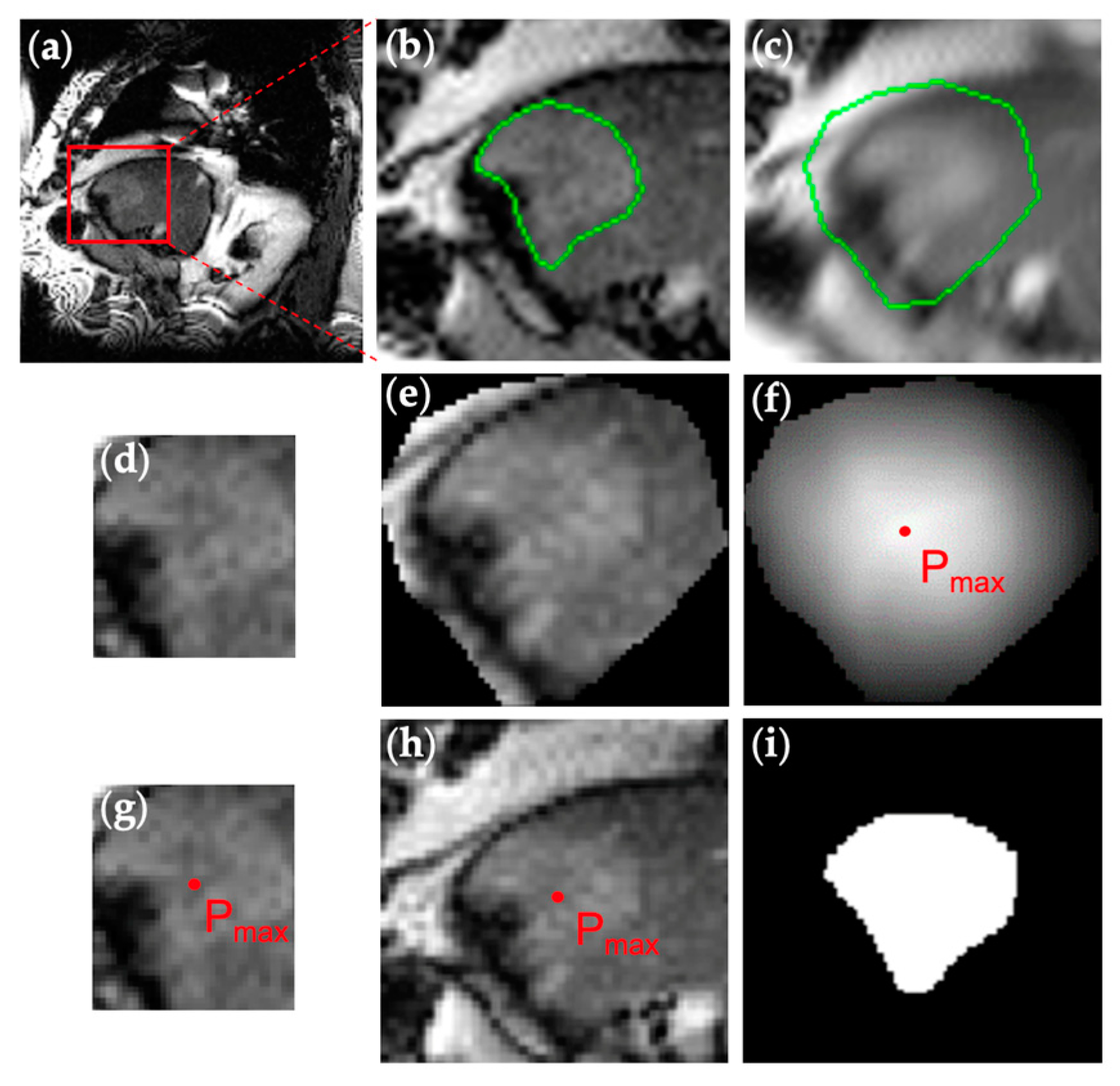
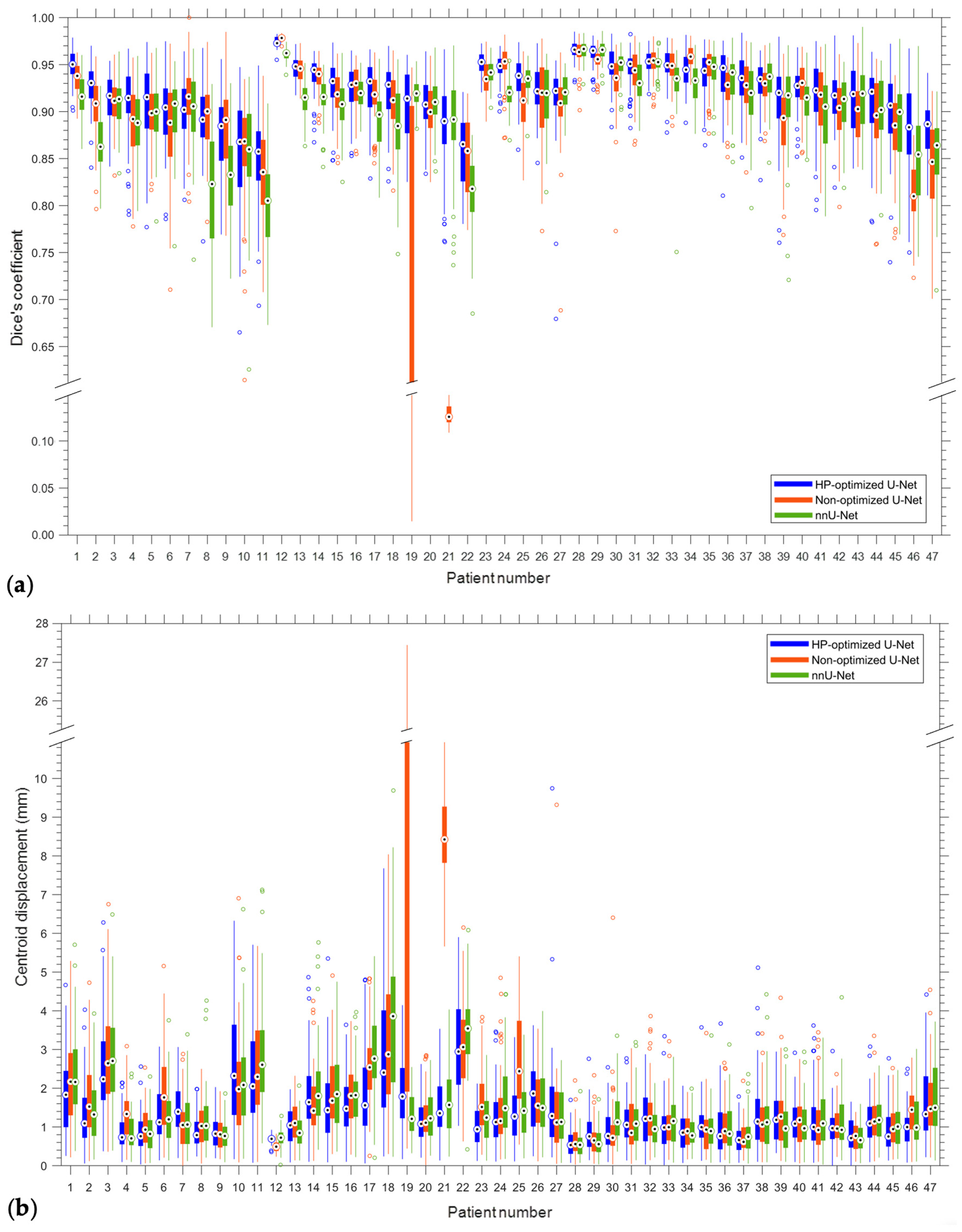
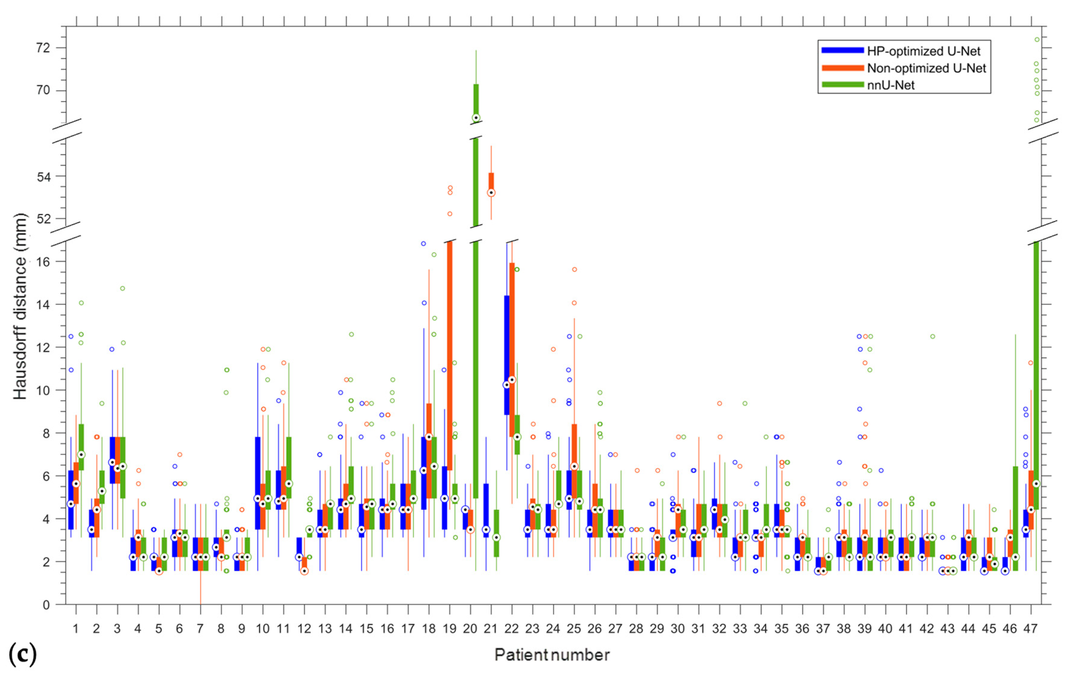
2.4. Performance Evaluation

The algorithm-generated autocontours (region of interest $(RO{I)}_{auto}$) from 70 testing images were evaluated by comparison with manual contours ($RO{I}_{manual}$) drawn by the experts. For quantitative comparison, three evaluation metrics were chosen based on the metric selection guidelines by Taha and Hanbury [63]. First, DC [48], defined as

$$DC=2{\displaystyle \frac{Area\left(RO{I}_{manual}\cap RO{I}_{auto}\right)}{Area\left(RO{I}_{manual}\right)+Area\left(RO{I}_{auto}\right)}}$$

(2)

was used, which provides an overlap-based measure of the agreement between two contours and, thus, is not sensitive to outlier segments [63]. For evaluating small segments, which are those with at least one dimension being significantly smaller (e.g., <5%) than the corresponding image dimension, distance-based metrics are recommended over overlap-based metrics [63]. As shown in Table 1, tumors of varying sizes were segmented in this study, and the tumors with a size < 5.1 cm² were considered as small segments based on the study by Taha and Hanbury [63]. Therefore, centroid displacement (CD) and Hausdorff distance (HD) [64] were also utilized to compensate for the shortcomings of DC, where CD is the separation between the centroid position of one contour and the other contour and HD is the maximum of all distances from a point in one contour to the closest point in the other contour. Each of these metrics was computed for 70 testing images per patient.

Furthermore, in order to benchmark the performance of the proposed HP-optimized U-Net, two widely established standards of neural networks for biomedical image segmentation were employed: U-Net [31] and nnU-Net [27], which are described in Section 2.4.1 and Section 2.4.2, respectively.

2.4.1. Non-Optimized U-Net

As the proposed method performs patient-specific HPO, it is essential to compare its performance against that of U-Net without HPO (called “non-optimized U-Net” hereinafter). Previously, Yun et al. [65] applied non-optimized U-Net (Figure 2) to segment tumors for some liver, prostate, and lung cancer patients. To improve speed, the original U-Net was modified while maintaining as similar an architecture as possible, by using image patches as input and two max-pooling operations. For training, 10,000 epochs, a learning rate of 1.0 × 10⁻⁴, and 30 training images were used, which were empirically found to perform well in general.

2.4.2. nnU-Net

nnU-Net (“no-new-Net”) [27] is a state-of-the-art segmentation method that has achieved the best performance on multiple benchmarks and challenges, proving its robustness and efficiency [26,27,32]. It is widely used for various segmentation tasks as a standardized baseline, a segmentation method, and a framework for developing novel segmentation methods [33,66]. nnU-Net is a self-adapting framework on the basis of 2D and 3D vanilla U-Nets. It automatically adapts to a given training dataset and configures a matching U-Net-based segmentation pipeline including network architecture, training, and post-processing. nnU-Net differs from U-Net in its architecture as it uses a leaky rectified linear unit (ReLU), instance normalization, and strided convolutions for down-sampling.

2.5. Overall Workflow

In summary, a potential clinical workflow for implementing the developed algorithm can be as follows:

• MR simulation to acquire dynamic images of a patient;
• Manual contouring of the tumor by experts in each dynamic image;
• Patient-specific HPO and training of the algorithm;
• Autocontouring during the actual treatment session.

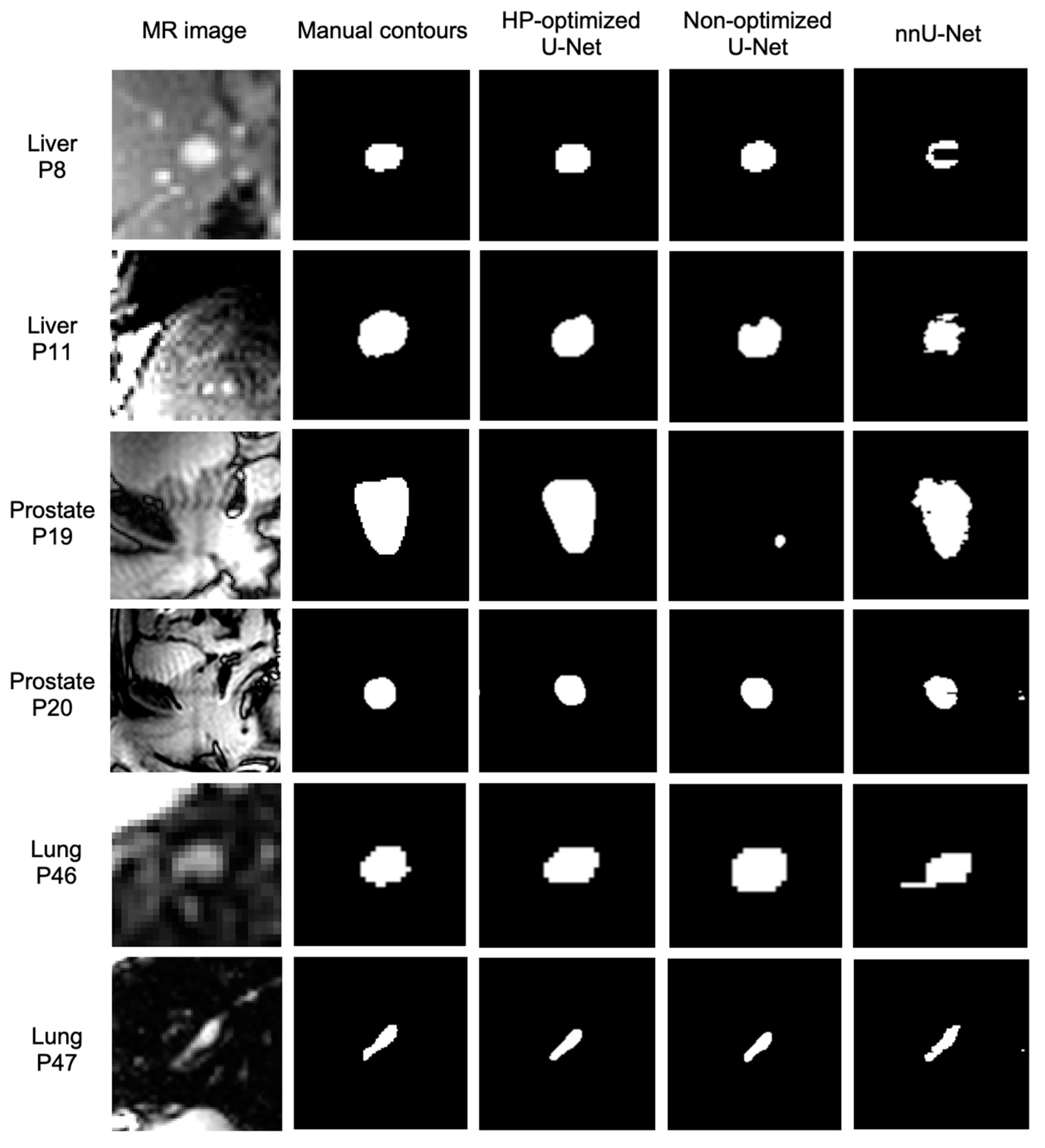
In step 1, an MR simulation takes place to acquire 130 dynamic images for a patient ~2 weeks prior to the actual treatment session (no motion management nor breathing guidance). In step 2, experts delineate the tumor in each dynamic image. The original 256 $\times$ 256 patient images are then cropped into small patches (~60 $\times$ 60) centered on the tumor to reduce the interference of background anatomy adjacent to the tumor and the number of computations. To create image patches for each patient dataset (example shown in Figure 3), prior to algorithm training, a single tumor contour (tumor ROI) that is the least impacted by motion artifacts during respiration is selected (often at the end of the exhale phase) from the 30 training images (Figure 3a,b). Also, a background region that represents the maximum anticipated range of tumor motion is delineated, by observing the tumor motion in the 30 training images (Figure 3c). Subsequently, the position of maximum cross correlation (P_max) is found using the normalized cross correlation operation between the tumor ROI and the background region in each image (Figure 3d–f). The tumor ROI centered at P_max is then dilated either 12 or 16 times (empirically chosen) to obtain image patches covering the possible variations in tumor size from deformation (Figure 3g–i). As a result, 130 image patches were generated.

In step 3, 60 consecutive image patches (30 for training, 30 for validation) and their corresponding manual contours are input into the CMA-ES optimization algorithm to search for the optimal set of hyperparameters. The U-Net, constructed and trained using the optimized hyperparameters, is evaluated by autocontouring the tumor in the remaining 70 testing images that were never seen by the algorithm. In step 4, the algorithm is used to autocontour the tumor in the actual treatment session. The algorithm consisting of HPO and autocontouring was coded in Pytorch version 1.6.0 on a 64-bit computer system (Ubuntu 18.04, Intel Core i9-7920X, 128 GB RAM) using the Python package, cma 2.7.0. The code will be available upon request for academic purposes. For faster execution of both HPO and the training of the algorithm, three graphics processing units (GPUs; NVIDIA GeForce RTX 2080 Ti) were utilized in parallel, while a single GPU was used for the final autocontouring.

3. Results

The HPO and training were performed together, as shown in Figure 1. The HP-optimized U-Net architecture for P46 is shown in Figure 4b as an example, along with the original U-Net architecture [31] in Figure 4a. P46 had the optimized hyperparameters that resulted in the simplest architecture of all cases. The optimized hyperparameters for the 47 patient cases are summarized in

Table A1. Optimized hyperparameters using CMA-ES for liver (P1–11), prostate (sagittal: P12–22, coronal: P23–27, axial: P28–35), and lung cancer patients (P36–47).

Patient		# of Convolutions	Filter Size	Feature Map #	# of Poolings	Learning Rate	# of Training Image Pairs
	Range:	1 or 2	3 or 5	[32, 128]	1 or 2	[10−5, 10−1]	[10, 30]
1		2	5	36	2	2.69 × 10−4	30
2		2	5	37	2	3.10 × 10−4	23
3		2	3	33	1	1.86 × 10−3	10
4		2	3	40	1	6.12 × 10−4	21
5		1	3	76	2	1.76 × 10−3	24
6		1	5	53	1	3.51 × 10−4	30
7		1	5	93	2	1.16 × 10−4	11
8		2	5	45	1	2.64 × 10−5	18
9		2	5	73	1	3.39 × 10−4	30
10		2	5	56	1	4.43 × 10−4	30
11		2	5	35	1	1.74 × 10−3	27
12		2	5	32	2	3.07 × 10−5	23
13		1	5	43	1	8.24 × 10−4	29
14		2	5	39	2	1.48 × 10−4	21
15		2	5	36	2	5.48 × 10−5	29
16		1	3	63	2	4.38 × 10−4	29
17		2	5	72	2	4.85 × 10−4	11
18		2	5	50	2	1.67 × 10−5	30
19		2	5	44	2	2.04 × 10−4	23
20		2	5	33	1	1.60 × 10−4	30
21		1	5	89	2	8.35 × 10−4	10
22		2	5	33	1	2.58 × 10−5	10
23		1	5	124	1	3.84 × 10−5	11
24		1	3	70	2	3.29 × 10−4	18
25		2	5	34	2	8.90 × 10−5	29
26		2	5	53	2	1.49 × 10−4	30
27		1	5	42	2	1.83 × 10−4	28
28		2	5	32	2	8.47 × 10−4	23
29		2	5	46	1	4.65 × 10−4	24
30		2	5	52	2	1.49 × 10−5	18
31		2	5	46	2	1.19 × 10−5	14
32		1	5	57	1	9.65 × 10−4	15
33		2	5	72	1	5.18 × 10−5	28
34		2	3	77	2	2.53 × 10−4	16
35		1	5	40	1	7.41 × 10−4	29
36		2	3	33	2	9.81 × 10−4	28
37		1	5	59	1	1.28 × 10−3	24
38		1	3	92	1	1.02 × 10−4	28
39		1	5	48	1	9.98 × 10−5	23
40		2	5	50	2	6.31 × 10−4	17
41		1	5	54	2	3.65 × 10−4	15
42		1	5	41	1	2.85 × 10−3	29
43		1	5	36	1	5.96 × 10−4	15
44		1	5	72	2	3.71 × 10−4	29
45		1	5	76	1	2.61 × 10−3	18
46		1	5	32	1	3.12 × 10−4	30
47		1	5	43	2	2.04 × 10−4	27

in Appendix A. The average time taken for HPO and the training of each patient case (i.e., execution time of Figure 1) ranged between 3 and 9 h, depending on the GPUs and version of Pytorch used (longer time using the authors’ workstation and shorter time using Colab with NVIDIA A100 GPU and Pytorch version 2.0.1).

The autocontours generated by the HP-optimized U-Net are visually compared against the manual contours for P1, 3, 4, 7–12, 16, 22, 24, 26–28, and 32 in Figure 5. In this figure, three sagittal (P12, 16, and 22), three coronal (P24, 26, and 27), and two axial (P28 and 32) prostate cases are shown as examples, where P12 and 22 are the cases with the highest and lowest mean DC of all prostate cases, respectively. It is important to emphasize that our algorithm was designed to mimic an individual expert’s manual contours, even if the contours are quite unique and not visually intuitive to others. The summary of the computed metrics for all patients is provided in

Table A2. Comparison between manual contours and autocontours generated by HP-optimized U-Net using Dice’s coefficient (DC), Intersection over Union (IoU), centroid displacement (CD), and Hausdorff distance (HD) for liver (P1–11), prostate (sagittal: P12–22, coronal: P23–27, axial: P28–35), and lung (P36–47) cancer patients (70 images/patient, SD: standard deviation).

Patient	DC		IoU		CD (mm)		HD (mm)
	Mean/SD	Max/Min	Mean/SD	Max/Min	Mean/SD	Max/Min	Mean/SD	Max/Min
1	0.95/0.02	0.98/0.90	0.90/0.03	0.96/0.82	1.84/1.00	4.67/0.25	4.96/1.77	12.50/3.13
2	0.93/0.02	0.97/0.84	0.86/0.04	0.94/0.72	1.29/0.81	4.03/0.06	3.49/0.75	4.94/1.56
3	0.91/0.03	0.95/0.84	0.84/0.04	0.91/0.73	2.47/1.29	6.28/0.37	6.67/1.82	11.90/3.49
4	0.91/0.04	0.97/0.79	0.84/0.06	0.94/0.65	0.87/0.48	2.14/0.09	2.25/0.71	4.42/1.56
5	0.91/0.04	0.97/0.78	0.84/0.07	0.95/0.64	0.85/0.50	2.56/0.03	2.08/0.61	3.49/1.56
6	0.90/0.04	0.97/0.79	0.82/0.06	0.95/0.65	1.31/0.74	3.07/0.14	3.10/1.18	6.44/1.56
7	0.90/0.03	0.96/0.81	0.82/0.05	0.93/0.68	1.44/0.62	3.06/0.20	2.31/0.74	4.69/1.56
8	0.89/0.04	0.97/0.76	0.81/0.06	0.94/0.62	0.88/0.45	1.98/0.24	2.64/0.81	4.69/1.56
9	0.88/0.05	0.96/0.77	0.79/0.07	0.92/0.63	0.88/0.42	2.03/0.19	2.11/0.62	3.49/1.56
10	0.86/0.06	0.95/0.67	0.75/0.09	0.90/0.50	2.51/1.45	6.33/0.17	5.58/2.24	11.27/1.56
11	0.85/0.05	0.95/0.69	0.74/0.07	0.90/0.53	2.30/1.35	5.71/0.08	5.26/1.58	9.50/2.21
12	0.97/0.01	0.98/0.96	0.95/0.01	0.97/0.91	0.69/0.11	0.93/0.35	2.51/0.52	3.13/1.56
13	0.95/0.01	0.97/0.92	0.90/0.02	0.95/0.85	1.05/0.47	1.97/0.08	3.84/1.06	6.99/1.56
14	0.94/0.02	0.96/0.87	0.89/0.03	0.93/0.77	1.82/0.93	4.87/0.10	4.53/1.37	9.88/3.13
15	0.93/0.03	0.97/0.85	0.87/0.04	0.95/0.74	1.56/0.96	5.35/0.09	3.97/1.44	9.38/1.56
16	0.92/0.03	0.96/0.85	0.86/0.04	0.93/0.74	1.55/0.80	3.64/0.10	4.43/1.15	8.84/2.21
17	0.92/0.03	0.97/0.83	0.86/0.05	0.93/0.71	1.88/1.24	4.80/0.06	4.64/1.33	7.97/3.13
18	0.92/0.03	0.97/0.83	0.86/0.05	0.94/0.70	2.81/1.68	7.68/0.24	6.68/2.87	16.83/2.21
19	0.91/0.04	0.96/0.83	0.83/0.06	0.92/0.70	1.88/0.90	4.15/0.17	5.30/1.75	10.94/3.13
20	0.91/0.03	0.96/0.83	0.83/0.05	0.93/0.72	1.14/0.57	2.62/0.21	3.92/0.91	5.63/2.21
21	0.89/0.05	0.97/0.76	0.80/0.08	0.93/0.61	1.57/0.85	3.53/0.13	3.93/1.50	7.81/1.56
22	0.86/0.04	0.92/0.78	0.75/0.06	0.85/0.64	3.10/1.21	5.90/1.03	11.52/3.75	24.41/6.25
23	0.95/0.01	0.97/0.92	0.91/0.02	0.95/0.85	1.02/0.57	2.12/0.12	3.76/0.82	6.44/2.21
24	0.95/0.02	0.97/0.90	0.90/0.03	0.94/0.82	1.29/0.77	3.46/0.11	4.00/1.20	7.97/2.21
25	0.94/0.02	0.97/0.86	0.88/0.04	0.95/0.75	1.37/0.75	3.32/0.11	5.38/1.96	12.50/3.13
26	0.92/0.02	0.97/0.85	0.86/0.04	0.95/0.73	1.82/0.88	3.63/0.24	3.82/1.13	6.25/1.56
27	0.92/0.04	0.95/0.68	0.84/0.06	0.91/0.51	1.52/1.33	9.75/0.21	3.90/1.83	17.19/2.21
28	0.97/0.01	0.99/0.93	0.93/0.02	0.97/0.87	0.58/0.34	1.70/0.07	2.13/0.56	3.49/1.56
29	0.96/0.01	0.98/0.92	0.93/0.02	0.96/0.86	0.84/0.48	2.76/0.14	2.22/0.77	4.69/1.56
30	0.95/0.02	0.98/0.88	0.90/0.04	0.97/0.79	0.94/0.56	2.54/0.09	3.22/0.96	6.99/1.56
31	0.95/0.02	0.98/0.88	0.90/0.04	0.97/0.79	1.13/0.55	2.77/0.13	3.21/1.00	6.25/1.56
32	0.95/0.01	0.98/0.92	0.91/0.02	0.95/0.85	1.28/0.72	2.88/0.03	4.42/1.06	6.63/3.13
33	0.95/0.02	0.98/0.88	0.90/0.03	0.96/0.78	0.99/0.59	3.34/0.1	2.65/0.89	6.63/1.56
34	0.94/0.02	0.98/0.89	0.89/0.03	0.96/0.80	0.89/0.49	2.06/0.07	3.30/0.89	5.63/1.56
35	0.94/0.03	0.98/0.86	0.89/0.04	0.95/0.76	1.07/0.56	3.57/0.12	4.04/1.26	7.81/2.21
36	0.94/0.03	0.98/0.81	0.88/0.05	0.95/0.68	0.95/0.68	3.67/0.09	2.33/0.75	4.69/1.56
37	0.93/0.03	0.98/0.85	0.88/0.05	0.97/0.74	0.70/0.38	1.79/0.08	1.86/0.48	3.13/1.56
38	0.93/0.03	0.97/0.83	0.87/0.04	0.93/0.71	1.34/0.92	5.11/0.10	2.87/1.00	6.63/1.56
39	0.93/0.10	0.98/0.76	0.84/0.06	0.96/0.61	1.50/2.31	19.85/0.32	2.87/2.14	12.50/1.56
40	0.92/0.02	0.97/0.85	0.86/0.04	0.94/0.74	1.13/0.57	2.92/0.09	2.63/0.79	6.25/1.56
41	0.92/0.04	0.98/0.80	0.85/0.06	0.95/0.66	1.18/0.77	3.62/0.08	2.26/0.73	4.69/1.56
42	0.92/0.03	0.98/0.82	0.85/0.05	0.96/0.69	1.01/0.50	2.96/0.00	2.41/0.63	4.42/1.56
43	0.91/0.04	0.98/0.84	0.84/0.07	0.96/0.72	0.80/0.43	1.65/0.00	1.60/0.21	3.13/1.56
44	0.91/0.04	0.96/0.78	0.84/0.06	0.93/0.64	1.14/0.57	3.07/0.09	2.32/0.80	4.69/1.56
45	0.90/0.04	0.97/0.74	0.82/0.07	0.95/0.59	0.93/0.57	2.77/0.13	1.97/0.57	3.13/1.56
46	0.88/0.05	0.97/0.75	0.79/0.08	0.95/0.61	1.00/0.49	2.50/0.08	1.81/0.45	3.13/1.56
47	0.88/0.03	0.94/0.81	0.79/0.05	0.89/0.68	1.60/0.95	4.42/0.22	3.71/1.52	9.11/1.56
Mean	0.92/0.04	0.97/0.83	0.85/0.05	0.94/0.71	1.35/1.03	3.95/0.15	3.63/2.17	7.51/2.01

in Appendix A.

Also, the DC, CD, and HD obtained using the HP-optimized U-Net, non-optimized U-Net, and nnU-Net are graphically compared in Figure 6. As patients were numbered in decreasing order of their mean DC for each site, this pattern of decreasing DC over patient number is seen in Figure 6a. The mean (SD) DC, CD, and HD of the 47 patient cases were 0.92 (0.04), 1.35 (1.03) mm, and 3.63 (2.17) mm, respectively, for HP-optimized U-Net; 0.89 (0.14), 1.85 (2.70) mm, and 5.23 (7.96) mm for non-optimized U-Net; and 0.90 (0.05), 1.44 (1.11) mm, and 5.16 (8.38) mm for nnU-Net. In addition, the DC, CD, and HD between the HP-optimized U-Net and the other two methods were compared using the paired t-test. A p-value smaller than 0.05 was considered to represent statistical significance.

Table 2. Number of patient cases (out of 47 patients) that showed statistical significance based on the paired t-test comparing HP-optimized U-Net with the standardized methods across the evaluation metrics. A p-value smaller than 0.05 was considered to represent statistical significance.

	Comparing HP-Optimized U-Net with Non-Optimized U-Net			Comparing HP-Optimized U-Net with nnU-Net
	# of Patients with Better Mean Value	# of Patients with p < 0.05		# of Patients with Better Mean Value	# of Patients with p < 0.05
		Two-Tailed	One-Tailed		Two-Tailed	One-Tailed
DC	36	33	32	37	31	30
CD	32	25	21	27	26	19
HD	32	26	24	39	37	33

shows the number of patient cases with p < 0.05 from two-tailed t-tests, as well as those from one-tailed t-tests (i.e., right-tailed for DC and left-tailed for CD and HD) out of the 47 patients. The number of patient cases with better mean values for the HP-optimized U-Net is also shown in this table for comparison. The results from the two-tailed t-tests show that the performance of the proposed method has statistically significant differences for the majority of patient cases, and thus, it can be distinguished from the other two methods. Similarly, the results from the one-tailed t-tests show that the improvements using the proposed method were statistically significant for the majority of patient cases in terms of DC and HD. Some example contours generated by each method are displayed in Figure 7. The patients shown in this figure are the cases that showed great differences in performance between different methods. For the methods with worse performance, contours varied considerably between images in the 70-testing-image set for some patients (e.g., P8 and 19). Thus, contours that deviated considerably from the manual contours and that were more representative of other contours in the set are shown in Figure 7. P8, 20, and 47 were the cases for which nnU-Net showed worse performance in terms of DC, CD, or HD. For P20 and 47, the small islands close to the right boundary were not removed by nnU-Net, resulting in very large HD values. P11 was the case in which all three methods did not perform well (lowest mean DC of all liver patients), P19 was the case in which non-optimized U-Net showed the worst performance, and P46 was the case in which both non-optimized U-Net and nnU-Net showed the worst performance. The mean (SD) autocontouring time per image of the 47 patients was found to be 54.2 (0.3) ms for HP-optimized U-Net, 55.6 (0.3) ms for non-optimized U-Net, and 4855 (610) ms for nnU-Net.

In

Table 3. Comparison of autocontouring performance for different HPO scenarios using training and validation datasets from various numbers of patients.

# of Patients Used for HPO	DC		CD (mm)		HD (mm)
	Mean/SD	Max/Min	Mean/SD	Max/Min	Mean/SD	Max/Min
(i) Patient-specific HPO	0.92/0.04	0.97/0.83	1.35/1.03	3.95/0.15	3.63/2.17	7.51/2.01
(ii) 30 patients (1 training and 1 validation image per patient)	0.64/0.05	0.77/0.53	7.34/2.35	13.28/3.14	15.81/3.53	24.31/9.95
(iii) 9 patients (30 training and 30 validation images per patient)	0.36/0.09	0.57/0.17	9.44/3.46	18.49/2.66	19.40/3.81	29.64/11.48
(iv) 15 patients (30 training and 30 validation images per patient)	0.47/0.07	0.63/0.33	8.54/3.32	16.03/3.29	17.03/4.09	25.96/9.59

, the autocontouring performance of the proposed algorithm using patient-specific HPO is compared with that of non-patient-specific HPO using four different scenarios: (i) patient-specific HPO as explained in Section 2.3; (ii)–(iv) non-patient-specific HPO; (ii) data of 30 randomly selected patients used for training (1 training and 1 validation image per patient); (iii) data of 9 randomly selected patients used for training, 3 patients per tumor site (30 training and 30 validation images per patient); and (iv) data of 15 randomly selected patients used for training, 5 patients per tumor site (30 training and 30 validation images per patient). In each scenario, testing was performed on 70 testing images for each of the 47 patients. The evaluation metrics comparing the generated autocontours against the manual contours in each scenario are shown in this table. Patient-specific HPO achieved the best overall contouring performance.

4. Discussion

NifteRT on linac-MR demands adequate tumor contouring accuracy, as well as contouring speed, which cannot be achieved by humans’ manual contouring. While automatization of tumor delineation using a deep neural network may provide a solution for this, finding the optimal set of hyperparameters of the network that results in satisfactory contouring performance remains a challenging problem. In this work, CMA-ES was implemented for patient-specific HPO within a U-Net-based autocontouring algorithm.

This study clearly demonstrates that the developed autocontouring routine is able to perform HPO to generate accurate autocontours for various patients that are comparable to experts’ manual contours. With the limited search ranges used in this study, the HP-optimized U-Net architecture for each patient was simpler than that of the original U-Net, as shown in Figure 4. In Figure 4b, the architecture was reduced by using one 5 $\times$ 5 convolution, 32 feature maps, and one pooling. The ability to autocontour with a simpler network architecture is beneficial as it leads to faster training and autocontouring with less demanding computing power. Overall, some general trends in the optimized hyperparameters were observed. For the number of convolutions, using one convolution was preferred for lung patients. For filter size, a strong preference for using 5 $\times$ 5 was observed for all patients. For learning rate, a relatively lower learning rate was preferred for prostate patients (e.g., median of 1.72 × 10⁻⁴ for prostate and 4.84 × 10⁻⁴ for lung). No trends were observed for the remaining hyperparameters. For the input range of the number of training images, annotating 30 images instead of 10 may not seem to dramatically increase the workload of a clinician. However, considering the total number of images that had to be annotated (i.e., 6110 images for 47 patients), this is a considerable increase in workload. Thus, reducing the number of training images as much as possible was the goal of its optimization. Also, the evaluation of autocontours revealed the overall promising contouring performance of the algorithm, which achieved a mean DC of ≥0.9 for all the studied patients except four liver patients (P8–11), two prostate patients (P21 and 22), and two lung patients (P46 and 47). P10 and 11 had relatively lower mean DCs of 0.86 and 0.85, respectively, which can be largely attributed to the fact that the tumors were hardly visible on the images. P22 also had a relatively lower mean DC of 0.86, which may be due to the pronounced artifacts on the images. The autocontouring performance was generally worse for liver patients than that for prostate patients because of the lower tumor contrast with the normal liver tissue background. For prostate patients, the sagittal (P12–22) and coronal cases (P23–27) were more challenging to contour than the axial cases (P28–35) due to the diffuse boundary of the prostate, and therefore, this mostly resulted in lower DC and higher CD and HD than those for the axial cases. Moreover, the algorithm was able to autocontour both P12 and P16 (or 22), which included and excluded seminal vesicles (SVs), respectively, in the contours. This suggests that the algorithm can accommodate varying clinical scenarios in which SVs may or may not be included in the treatment volume. If SVs are excluded, autocontouring becomes more challenging as there is no visible boundary between the prostate and SVs.

Comparing the three segmentation methods, HP-optimized U-Net achieved the best overall contouring performance in terms of all three evaluation metrics, while non-optimized U-Net showed the worst performance. Despite the fact that both non-optimized U-Net and nnU-Net achieved mean DC values comparable to the intra- and interobserver DC values, their mean HD values were both larger than the intra- and interobserver HD values of 4.3 (1.7) and 4.7 (1.6) mm [49]. The contours from nnU-Net mostly included holes, ragged edges, and/or small islands. nnU-Net applies post-processing, i.e., removing small islands, only if the DC of its contours on the validation images is improved by removing those islands [27]. As there were no small islands found in the validation results, post-processing was not applied to the testing images, resulting in the observed islands. Although applying post-processing ourselves would improve its performance for these cases, the results were left as they were for a fair comparison of the three methods. Furthermore, as can be seen in Figure 6 and Figure 7, contours by non-optimized U-Net for P19 and 21 largely deviated from the manual contours and differed considerably from those of the other two methods. Considering that the autocontouring accuracies in the training images for these patients were much higher (~0.9 DC) than the accuracies in testing images, the network might have overfit to the training images because non-optimized U-Net did not utilize early stopping. Employing a regularization technique such as early stopping may improve its performance for these patients. For autocontouring speed, HP-optimized U-Net was the fastest method while nnU-Net was the slowest. The large difference in inference time between nnU-Net and the other two methods may have come from the fact that nnU-Net additionally performed test time augmentation, which was applied by mirroring along all axes, as well as instance normalization, which was applied after each convolution. Also, nnU-Net used whole images as input, while image patches were used in the other two methods. Using whole images as input results in performing more matrix computations (during operations such as convolutions) in the network, which may lead to prolonged inference time.

The autocontouring time of HP-optimized U-Net was 54.2 ms for each dynamic image. The American Association of Physicists in Medicine (AAPM) Task Group 76 report recommends a maximum delay time of 500 ms for real-time tumor tracking [67]. This delay includes times for image acquisition, reconstruction, contouring, and MLC repositioning. With the rate of intrafractional 2D MR imaging of linac-MR being 4 frames/s (i.e., 250 ms per frame), 54.2 ms is within the clinically feasible range. The autocontouring time, along with the time taken for HPO, can be further reduced using higher-end hardware and optimized coding technique and GPU performance. Studies have shown that an autocontouring time of 1–25 ms is also possible on standard workstation computers [24,68]. Additionally, even though the HPO of each patient takes 3–9 h on average, this will be performed several days prior to the actual treatment, allowing the autocontouring algorithm to be ready for use at the time of the treatment. In clinical practice, typically ~2 weeks of treatment planning is allowed before treatment, assuming no drastic anatomical change takes place during this period. As treatment is replanned in the case of large anatomical changes, HPO will also be performed again in this case using updated patient images.

One limitation of this study is that the patients were imaged on a 3 T MRI system although a linac-MR system, which typically operates at a lower field strength (B₀) [17,18,19,20,69]. Hence, the quality of the images obtained with linac-MR will be different, which may result in different contouring performance of the algorithm. The ability to distinguish a tumor from tissue background during nifteRT largely depends on contrast-to-noise ratio (CNR) between the two, which is known to be affected by B₀ [70]. While there is a complex relationship between CNR and B₀, studies have shown better image contrast using a lower B₀ (e.g., 0.55 T) for sites including the liver and lung, provided that the MRI system is equipped with state-of-the-art hardware [70,71]. This suggests that the contouring performance of our algorithm on the images acquired by a linac-MR system may be comparable to that presented in this study. In addition, other factors such as the MRI sequence, scan parameters, and presence of image artifacts can all affect image quality and the contouring performance of the algorithm. However, despite the pronounced artifacts shown in the P22 and P24 images in Figure 5, the algorithm was able to autocontour with reasonable accuracy. This suggests solid performance of the algorithm even in the presence of artifacts. Another limitation of this study is that there can be through-plane tumor motion that is not captured by the 2D MR images. During the 2D imaging of a mobile tumor on the linac-MR, the imaging plane will be oriented to include the two major axes of tumor motion. This will allow the detection of any in-plane changes in tumor shape and position. For handling any potential through-plane motion, one possible solution is adjusting the slice thickness of the imaging plane to ensure that the tumor remains in the imaging plane. This issue can also be addressed by acquiring a 3D image volume, which can be achieved by using accelerated imaging techniques such as parallel imaging, compressed sensing, and neural network reconstructions [72,73,74]. Moreover, studies have shown that 2D multi-slice or orthogonal imaging can capture the 3D motion of mobile tumors [75,76,77].

Although the developed algorithm achieved the goal of a mean DC of ≥0.9 for most patient cases, there is still room for improvement as CD and HD for some of those cases were large; for example, maximum CD was 19.85 mm in P39 and maximum HD was 24.41 mm in P22. These can be further improved in various ways. For optimizations by CMA-ES, a fixed population size of 10 was used in this work. However, due to the nature of CMA-ES, using a varying population size over the course of the search may improve the optimizations. This is because using a small population size often leads to faster convergence but may lead to solutions being stuck in local minima by failing to explore various minima with diverse solutions, whereas using a large population helps to prevent being stuck in local minima for a more global search, but the search may be too slow until convergence. Also, optimizing more hyperparameters such as activation function and sampling distribution for initial weights could result in better contouring accuracy. Furthermore, contouring performance can be improved by adopting a different model architecture. U-Net uses concatenations to combine shallow, low-level, fine-grained feature maps from the encoder with deep, semantic, coarse-grained feature maps from the decoder. The fusion of semantically dissimilar feature maps using plain concatenations in U-Net can make the learning task difficult for the network. This semantic gap between the encoder and decoder can be reduced by employing variants of U-Net, such as U-Net++ [78] or U-Net3+ [79], which use nested, dense concatenations and redesigned concatenations to combine multi-scale feature maps, respectively. Moreover, convolutional neural network-based models such as U-Net have a limitation in that it may not be good at capturing long-range spatial relations present in an image due to the intrinsic locality of convolution operations. This can be overcome by employing a vision transformer [80], which is known to be powerful at extracting long-range relations by using its self-attention mechanism. Although exploring more advanced architectures may enhance contouring performance, it is essential to carefully monitor computational time, as the ultimate goal is to enable real-time autocontouring. Achieving an optimal balance between accuracy and speed is critical to meeting the requirements of nifteRT.

5. Conclusions

For nifteRT, an autocontouring routine has been developed by implementing HPO with CMA-ES in a U-Net-based algorithm, and its contouring accuracy and speed were validated using in vivo MR images of 47 liver, prostate, and lung cancer patients. By optimizing six hyperparameters for each patient case, the algorithm achieved a DC, CD, and HD of 0.92 (0.04), 1.35 (1.03) mm, and 3.63 (2.17) mm, respectively, between the manual contours and autocontours averaged over all the patients. The developed routine allows for patient-specific HPO, leading to adequate autocontouring performance that may be comparable to that of human experts.

References

1. Huang, F.; Ma, C.; Wang, R.; Gong, G.; Shang, D.; Yin, Y. Defining the individual internal gross tumor volume of hepatocellular carcinoma using 4DCT and T2-weighted MRI images by deformable registration. Transl. Cancer Res. 2018, 7, 151–157. [Google Scholar] [CrossRef]
2. Feng, M.; Balter, J.M.; Normolle, D.; Adusumilli, S.; Cao, Y.; Chenevert, T.L.; Ben-Josef, E. Characterization of pancreatic tumor motion using cine MRI: Surrogates for tumor position should be used with caution. Int. J. Radiat. Oncol. Biol. Phys. 2009, 74, 884–891. [Google Scholar] [CrossRef]
3. Kyriakou, E.; McKenzie, D.R. Changes in lung tumor shape during respiration. Phys. Med. Biol. 2012, 57, 919–935. [Google Scholar] [CrossRef]
4. Sawant, A.; Venkat, R.; Srivastava, V.; Carlson, D.; Povzner, S.; Cattell, H.; Keall, P. Management of three-dimensional intrafraction motion through real-time DMLC tracking. Med. Phys. 2008, 35, 2050–2061. [Google Scholar] [CrossRef] [PubMed]
5. Willoughby, T.; Lehmann, J.; Bencomo, J.A.; Jani, S.K.; Santanam, L.; Sethi, A.; Solberg, T.D.; Tome, W.A.; Waldron, T.J. Quality assurance for nonradiographic radiotherapy localization and positioning systems: Report of Task Group 147. Med. Phys. 2012, 39, 1728–1747. [Google Scholar] [CrossRef]
6. Bertholet, J.; Knopf, A.; Eiben, B.; McClelland, J.; Grimwood, A.; Harris, E.; Menten, M.; Poulsen, P.; Nguyen, D.T.; Keall, P.; et al. Real-time intrafraction motion monitoring in external beam radiotherapy. Phys. Med. Biol. 2019, 64, 15TR01. [Google Scholar] [CrossRef] [PubMed]
7. Schweikard, A.; Shiomi, H.; Adler, J. Respiration tracking in radiosurgery. Med. Phys. 2004, 31, 2738–2741. [Google Scholar] [CrossRef]
8. Matsuo, Y.; Ueki, N.; Takayama, K.; Nakamura, M.; Miyabe, Y.; Ishihara, Y.; Mukumoto, N.; Yano, S.; Tanabe, H.; Kaneko, S.; et al. Evaluation of dynamic tumour tracking radiotherapy with real-time monitoring for lung tumours using a gimbal mounted linac. Radiother. Oncol. 2014, 112, 360–364. [Google Scholar] [CrossRef]
9. Depuydt, T.; Poels, K.; Verellen, D.; Engels, B.; Collen, C.; Buleteanu, M.; Van den Begin, R.; Boussaer, M.; Duchateau, M.; Gevaert, T.; et al. Treating patients with real-time tumor tracking using the Vero gimbaled linac system: Implementation and first review. Radiother. Oncol. 2014, 112, 343–351. [Google Scholar] [CrossRef]
10. D’Souza, W.D.; Naqvi, S.A.; Yu, C.X. Real-time intra-fraction-motion tracking using the treatment couch: A feasibility study. Phys. Med. Biol. 2005, 50, 4021–4033. [Google Scholar] [CrossRef]
11. Cho, B.; Poulsen, P.R.; Sloutsky, A.; Sawant, A.; Keall, P.J. First demonstration of combined kV/MV image-guided real-time dynamic multileaf-collimator target tracking. Int. J. Radiat. Oncol. Biol. Phys. 2009, 74, 859–867. [Google Scholar] [CrossRef] [PubMed]
12. Glitzner, M.; Woodhead, P.L.; Borman, P.T.S.; Lagendijk, J.J.W.; Raaymakers, B.W. Technical note: MLC-tracking performance on the Elekta unity MRI-linac. Phys. Med. Biol. 2019, 64, 15NT02. [Google Scholar] [CrossRef]
13. Keall, P.J.; Sawant, A.; Berbeco, R.I.; Booth, J.T.; Cho, B.; Cerviño, L.I.; Cirino, E.; Dieterich, S.; Fast, M.F.; Greer, P.B.; et al. AAPM Task Group 264: The safe clinical implementation of MLC tracking in radiotherapy. Med. Phys. 2021, 48, e44–e64. [Google Scholar] [CrossRef] [PubMed]
14. Kitamura, K.; Shirato, H.; Shimizu, S.; Shinohara, N.; Harabayashi, T.; Shimizu, T.; Kodama, Y.; Endo, H.; Onimaru, R.; Nishioka, S.; et al. Registration accuracy and possible migration of internal fiducial gold marker implanted in prostate and liver treated with real-time tumor-tracking radiation therapy (RTRT). Radiother. Oncol. 2002, 62, 275–281. [Google Scholar] [CrossRef] [PubMed]
15. Ionascu, D.; Jiang, S.B.; Nishioka, S.; Shirato, H.; Berbeco, R.I. Internal-external correlation investigations of respiratory induced motion of lung tumors. Med. Phys. 2007, 34, 3893–3903. [Google Scholar] [CrossRef]
16. Gierga, D.P.; Brewer, J.; Sharp, G.C.; Betke, M.; Willett, C.G.; Chen, G.T. The correlation between internal and external markers for abdominal tumors: Implications for respiratory gating. Int. J. Radiat. Oncol. Biol. Phys. 2005, 61, 1551–1558. [Google Scholar] [CrossRef]
17. Fallone, B.G.; Murray, B.; Rathee, S.; Stanescu, T.; Steciw, S.; Vidakovic, S.; Blosser, E.; Tymofichuk, D. First MR images obtained during megavoltage photon irradiation from a prototype integrated linac-MR system. Med. Phys. 2009, 36, 2084–2088. [Google Scholar] [CrossRef]
18. Fallone, B.G. The rotating biplanarlinac magnetic resonance imaging system. Semin. Radiat. Oncol. 2014, 24, 200–202. [Google Scholar] [CrossRef]
19. Mutic, S.; Dempsey, J.F. The ViewRay system: Magnetic resonance-guided and controlled radiotherapy. Semin. Radiat. Oncol. 2014, 24, 196–199. [Google Scholar] [CrossRef]
20. Raaymakers, B.W.; Lagendijk, J.J.W.; Overweg, J.; Kok, J.G.M.; Raaijmakers, A.J.E.; Kerkhof, E.M.; van der Put, R.W.; Meijsing, I.; Crijins, S.P.M.; Benedosso, F.; et al. Integrating a 1.5 T MRI scanner with a 6 MV accelerator: Proof of concept. Phys. Med. Biol. 2009, 54, N229. [Google Scholar] [CrossRef]
21. Yun, J.; Wachowicz, K.; Mackenzie, M.; Rathee, S.; Robinson, D.; Fallone, B.G. First demonstration of intrafractional tumor-tracked irradiation using 2D phantom MR images on a prototype linac-MR. Med. Phys. 2013, 40, 051718. [Google Scholar] [CrossRef] [PubMed]
22. Cerviño, L.I.; Du, J.; Jiang, S.B. MRI-guided tumor tracking in lung cancer radiotherapy. Phys. Med. Biol. 2011, 56, 3773–3785. [Google Scholar] [CrossRef]
23. Uijtewaal, P.; Borman, P.T.S.; Woodhead, P.L.; Hackett, S.L.; Raaymakers, B.W.; Fast, M.F. Dosimetric evaluation of MRI-guided multi-leaf collimator tracking and trailing for lung stereotactic body radiation therapy. Med. Phys. 2021, 48, 1520–1532. [Google Scholar] [CrossRef]
24. Yun, J.; Yip, E.; Gabos, Z.; Wachowicz, K.; Rathee, S.; Fallone, B.G. Neural-network based autocontouring algorithm for intrafractional lung-tumor tracking using Linac-MR. Med. Phys. 2015, 42, 2296–2310. [Google Scholar] [CrossRef] [PubMed]
25. Hansen, N.; Ostermeier, A. Completely Derandomized Self-Adaptation in Evolution Strategies. Evol. Comput. 2001, 9, 159–195. [Google Scholar] [CrossRef] [PubMed]
26. Antonelli, M.; Reinke, A.; Bakas, S.; Farahani, K.; Kopp-Schneider, A.; Landman, B.A.; Litjens, G.; Menze, B.; Ronneberger, O.; Summers, R.M.; et al. The Medical Segmentation Decathlon. Nat. Commun. 2022, 13, 4128. [Google Scholar] [CrossRef]
27. Isensee, F.; Jaeger, P.F.; Kohl, S.A.A.; Petersen, J.; Maier-Hein, K.H. nnU-Net: A self-configuring method for deep learning-based biomedical image segmentation. Nat. Methods 2021, 18, 203–211. [Google Scholar] [CrossRef]
28. Long, J.; Shelhamer, E.; Darrell, T. Fully convolutional networks for semantic segmentation. In Proceedings of the IEEE Conference on Computer Vision and Pattern Recognition (CVPR), Boston, MA, USA, 7–12 June 2015; pp. 3431–3440. [Google Scholar] [CrossRef]
29. Minaee, S.; Boykov, Y.; Porikli, F.; Plaza, A.; Kehtarnavaz, N.; Terzopoulos, D. Image segmentation using deep learning: A survey. IEEE Trans. Pattern Anal. Mach. Intell. 2022, 44, 3523–3542. [Google Scholar] [CrossRef]
30. Liu, W.; Rabinovich, A.; Berg, A.C. ParseNet: Looking wider to see better. arXiv 2015, arXiv:1506.04579. [Google Scholar]
31. Ronneberger, O.; Fischer, P.; Brox, T. U-net: Convolutional networks for biomedical image segmentation. In Proceedings of the Medical Image Computing and Computer-Assisted Intervention–MICCAI 2015: 18th International Conference, Munich, Germany, 5–9 October 2015; Proceedings, Part III 18. Springer: Berlin/Heidelberg, Germany, 2015; pp. 234–241. [Google Scholar] [CrossRef]
32. Bilic, P.; Christ, P.; Li, H.B.; Vorontsov, E.; Ben-Cohen, A.; Kaissis, G.; Szeskin, A.; Jacobs, C.; Mamani, G.E.H.; Chartrand, G.; et al. The Liver Tumor Segmentation Benchmark (LiTS). Med. Image Anal. 2023, 84, 102680. [Google Scholar] [CrossRef]
33. Pedrosa, J.; Aresta, G.; Ferreira, C.; Atwal, G.; Phoulady, H.A.; Chen, X.; Chen, R.; Li, J.; Wang, L.; Galdran, A.; et al. LNDb challenge on automatic lung cancer patient management. Med. Image Anal. 2021, 70, 102027. [Google Scholar] [CrossRef] [PubMed]
34. Loshchilov, I.; Hutter, F. CMA-ES for hyperparameter optimization of deep neural networks. arXiv 2016, arXiv:1604.07269. [Google Scholar]
35. Aggarwal, C.C. Neural Networks and Deep Learning: A Textbook, 1st ed.; Springer International Publishing: Yorktown, VA, USA, 2018; pp. 139–191. [Google Scholar] [CrossRef]
36. Loshchilov, I.; Schoenauer, M.; Sebag, M. Bi-population CMA-ES algorithms with surrogate models and line searches. In Proceedings of the 15th Annual Conference on Genetic and Evolutionary Computation, Amsterdam, The Netherlands, 6–10 July 2013; pp. 1177–1184. [Google Scholar] [CrossRef]
37. Wollmann, T.; Bernhard, P.; Gunkel, M.; Braun, D.M.; Meiners, J.; Simon, R.; Sauter, G.; Erfle, H.; Rippe, K.; Rohr, K. Black-Box Hyperparameter Optimization for Nuclei Segmentation in Prostate Tissue Images. In Bildverarbeitung Für Die Medizin 2019; Handels, H., Deserno, T., Maier, A., Maier-Hein, K., Palm, C., Tolxdorff, T., Eds.; Springer Vieweg: Wiesbaden, Germany, 2019; pp. 345–350. [Google Scholar] [CrossRef]
38. Tsai, Y.L.; Wu, C.J.; Shaw, S.; Yu, P.C.; Nien, H.H.; Lui, L.T. Quantitative analysis of respiration-induced motion of each liver segment with helical computed tomography and 4-dimensional computed tomography. Radiat. Oncol. 2018, 13, 59. [Google Scholar] [CrossRef] [PubMed]
39. Shirato, H.; Seppenwoolde, Y.; Kitamura, K.; Onimura, R.; Shimizu, S. Intrafractional tumor motion: Lung and liver. Semin. Radiat. Oncol. 2004, 14, 10–18. [Google Scholar] [CrossRef]
40. Plathow, C.; Fink, C.; Ley, S.; Puderbach, M.; Eichinger, M.; Zuna, I.; Schmähl, A.; Kauczor, H.U. Measurement of tumor diameter-dependent mobility of lung tumors by dynamic MRI. Radiother. Oncol. 2004, 73, 349–354. [Google Scholar] [CrossRef]
41. Huang, E.; Dong, L.; Chandra, A.; Kuban, D.A.; Rosen, I.I.; Evans, A.; Pollack, A. Intrafraction prostate motion during IMRT for prostate cancer. Int. J. Radiat. Oncol. Biol. Phys. 2002, 53, 261–268. [Google Scholar] [CrossRef]
42. Gurjar, O.P.; Arya, R.; Goyal, H. A study on prostate movement and dosimetric variation because of bladder and rectum volumes changes during the course of image-guided radiotherapy in prostate cancer. Prostate Int. 2020, 8, 91–97. [Google Scholar] [CrossRef]
43. Deasy, J.O.; Blanco, A.I.; Clark, V.H. CERR: A computational environment for radiotherapy research. Med. Phys. 2003, 30, 979–985. [Google Scholar] [CrossRef]
44. Fedorov, A.; Beichel, R.; Kalpathy-Cramer, J.; Finet, J.; Fillion-Robin, J.C.; Pujol, S.; Bauer, C.; Jennings, D.; Fennessy, F.; Sonka, M.; et al. 3D Slicer as an image computing platform for the quantitative imaging network. Magn. Reson. Imaging 2012, 30, 1323–1341. [Google Scholar] [CrossRef]
45. Smolders, A.; Lomax, A.; Weber, D.C.; Albertini, F. Patient-specific neural networks for contour propagation in online adaptive radiotherapy. Phys. Med. Biol. 2023, 68, 095010. [Google Scholar] [CrossRef]
46. Jansen, M.J.A.; Kuijf, H.J.; Dhara, A.K.; Weaver, N.A.; Jan Biessels, G.; Strand, R.; Pluim, J.P.W. Patient-specific fine-tuning of convolutional neural networks for follow-up lesion quantification. J. Med. Imaging 2020, 7, 064003. [Google Scholar] [CrossRef]
47. Fransson, S.; Tilly, D.; Strand, R. Patient specific deep learning based segmentation for magnetic resonance guided prostate radiotherapy. Phys. Imaging Radiat. Oncol. 2022, 23, 38–42. [Google Scholar] [CrossRef] [PubMed]
48. Dice, L.R. Measures of the amount of ecologic association between species. Ecology 1945, 26, 297–302. [Google Scholar] [CrossRef]
49. Yip, E.; Yun, J.; Gabos, Z.; Baker, S.; Yee, D.; Wachowicz, K.; Rathee, S.; Fallone, B.G. Evaluating performance of a user-trained MR lung tumor autocontouring algorithm in the context of intra- and interobserver variations. Med. Phys. 2018, 45, 307–313. [Google Scholar] [CrossRef] [PubMed]
50. Zeng, G.; Yang, X.; Li, J.; Yu, L.; Heng, P.; Zheng, G. 3D U-net with Multi-level Deep Supervision: Fully Automatic Segmentation of Proximal Femur in 3D MR Images. In Machine Learning in Medical Imaging; Wang, Q., Shi, Y., Suk, H.I., Suzuki, K., Eds.; Springer: Cham, Switzerland, 2017; pp. 274–282. [Google Scholar] [CrossRef]
51. Jia, S.; Despinasse, A.; Wang, Z.; Delingette, H.; Pennec, X.; Jaïs, P.; Cochet, H.; Sermesant, M. Automatically segmenting the left atrium from cardiac images using successive 3D U-nets and a contour loss. arXiv 2018, arXiv:1812.02518. [Google Scholar]
52. Huang, Q.; Sun, J.; Ding, H.; Wang, X.; Wang, G. Robust liver vessel extraction using 3D U-Net with variant dice loss function. Comput. Biol. Med. 2018, 101, 153–162. [Google Scholar] [CrossRef]
53. Saleh, H.M.; Saad, N.H.; Isa, N.A.M. Overlapping Chromosome Segmentation using U-Net: Convolutional Networks with Test Time Augmentation. Procedia Comput. Sci. 2019, 159, 524–533. [Google Scholar] [CrossRef]
54. Yang, J.; Faraji, M.; Basu, A. Robust segmentation of arterial walls in intravascular ultrasound images using Dual Path U-Net. Ultrasonics 2019, 96, 24–33. [Google Scholar] [CrossRef]
55. Tchito Tchapga, C.; Mih, T.A.; Tchagna Kouanou, A.; Fozin Fonzin, T.; Kuetche Fogang, P.; Mezatio, B.A.; Tchiotsop, D. Biomedical Image Classification in a Big Data Architecture Using Machine Learning Algorithms. J. Healthc. Eng. 2021, 2021, 9998819. [Google Scholar] [CrossRef]
56. Kim, B.; Yu, K.; Lee, P. Cancer classification of single-cell gene expression data by neural network. Bioinformatics 2020, 36, 1360–1366. [Google Scholar] [CrossRef]
57. Siddique, N.; Sidike, P.; Colin, E.; Devabhaktuni, V. U-Net and Its Variants for Medical Image Segmentation: A Review of Theory and Applications. IEEE Access 2021, 9, 82031–82057. [Google Scholar] [CrossRef]
58. Feurer, M.; Hutter, F. Chapter 1: Hyperparameter Optimization. In Automated Machine Learning: Methods, Systems, Challenges; Hutter, F., Kotthoff, L., Vanschoren, J., Eds.; Springer: Cham, Switzerland, 2019; pp. 3–33. [Google Scholar]
59. Greff, K.; Srivastava, R.K.; Koutník, J.; Steunebrink, B.R.; Schmidhuber, J. LSTM: A Search Space Odyssey. IEEE Trans. Neural Netw. Learn. Syst. 2015, 28, 2222–2232. [Google Scholar] [CrossRef]
60. Masood, D.A. Automated Machine Learning Hyperparameter Optimization Neural Architecture Search and Algorithm Selection with Cloud Platforms; Packt Publishing Ltd.: Birmingham, UK, 2021; pp. 27–30. [Google Scholar]
61. Wu, J.; Chen, X.Y.; Zhang, H.; Xiong, L.D.; Lei, H.; Deng, S.H. Hyperparameter Optimization for Machine Learning Models Based on Bayesian Optimization. J. Electron. Sci. Technol. 2019, 17, 26–40. [Google Scholar] [CrossRef]
62. Kingma, D.; Ba, J.L. Adam: A Method for Stochastic Optimization. arXiv 2014, arXiv:1412.6980. [Google Scholar]
63. Taha, A.A.; Hanbury, A. Metrics for evaluating 3D medical image segmentation: Analysis, selection, and tool. BMC Med. Imaging 2015, 15, 29. [Google Scholar] [CrossRef] [PubMed]
64. Huttenlocher, D.P.; Klanderman, G.A.; Rucklidge, W.J. Comparing images using the Hausdorff distance. IEEE Trans. Pattern Anal. Mach. Intell. 1993, 15, 850–863. [Google Scholar] [CrossRef]
65. Yun, J.; Yip, E.; Gabos, Z.; Usmani, N.; Yee, D.; Wachowicz, K.; Fallone, B.G. An AI-based tumor autocontouring algorithm for non-invasive intra-fractional tumor-tracked radiotherapy (nifteRT) on linac-MR. Med. Phys. 2020, 47, e576. [Google Scholar]
66. Ma, J. Cutting-edge 3d medical image segmentation methods in 2020: Are happy families all alike? arXiv 2021, arXiv:2101.00232. [Google Scholar]
67. Keall, P.J.; Mageras, G.S.; Balter, J.M.; Emery, R.S.; Forster, K.M.; Jiang, S.B.; Kapatoes, J.M.; Low, D.A.; Murphy, M.J.; Murray, B.R.; et al. The management of respiratory motion in radiation oncology report of AAPM Task Group 76. Med. Phys. 2006, 33, 3874–3900. [Google Scholar] [CrossRef]
68. Fast, M.F.; Eiben, B.; Menten, M.J.; Wetscherek, A.; Hawkes, D.J.; McClelland, J.R.; Oelfke, U. Tumor auto-contouring on 2d cine MRI for locally advanced lung cancer: A comparative study. Radiother. Oncol. 2017, 125, 485–491. [Google Scholar] [CrossRef]
69. Klüter, S. Technical design and concept of a 0.35 T MR-Linac. Clin. Transl. Radiat. Oncol. 2019, 18, 98–101. [Google Scholar] [CrossRef]
70. Wachowicz, K.; De Zanche, N.; Yip, E.; Volotovskyy, V.; Fallone, B.G. CNR considerations for rapid real-time MRI tumor tracking in radiotherapy hybrid devices: Effects of B0 field strength. Med. Phys. 2016, 43, 4903. [Google Scholar] [CrossRef] [PubMed]
71. Campbell-Washburn, A.E.; Ramasawmy, R.; Restivo, M.C.; Bhattacharya, I.; Basar, B.; Herzka, D.A.; Hansen, M.S.; Rogers, T.; Bandettini, W.P.; McGuirt, D.R.; et al. Opportunities in interventional and diagnostic imaging by using high-performance low-field-strength MRI. Radiology 2019, 293, 384–393. [Google Scholar] [CrossRef]
72. Yip, E.; Yun, J.; Wachowicz, K.; Gabos, Z.; Rathee, S.; Fallone, B.G. Sliding window prior data assisted compressed sensing for MRI tracking of lung tumors. Med. Phys. 2017, 44, 84–98. [Google Scholar] [CrossRef]
73. Kim, T.; Park, J.C.; Gach, H.M.; Chun, J.; Mutic, S. Technical note: Realtime 3D MRI in the presence of motion for MRI-guided radiotherapy: 3D dynamic keyhole imaging with super-resolution. Med. Phys. 2019, 46, 4631–4638. [Google Scholar] [CrossRef] [PubMed]
74. Terpstra, M.L.; Maspero, M.; D’Agata, F.; Stemkens, B.; Intven, M.P.W.; Lagendijk, J.J.W.; van den Berg, C.A.T.; Tijssen, R.H.N. Deep learning-based image reconstruction and motion estimation from undersampled radial k-space for real-time MRI-guided radiotherapy. Phys. Med. Biol. 2020, 65, 155015. [Google Scholar] [CrossRef]
75. Ginn, J.S.; Low, D.A.; Lamb, J.M.; Ruan, D. A motion prediction confidence estimation framework for prediction-based radiotherapy gating. Med. Phys. 2020, 47, 3297–3304. [Google Scholar] [CrossRef] [PubMed]
76. Bjerre, T.; Crijns, S.; af Rosenschöld, P.M.; Aznar, M.; Specht, L.; Larsen, R.; Keall, P. Three-dimensional MRI-linac intra-fraction guidance using multiple orthogonal cine-MRI planes. Phys. Med. Biol. 2013, 58, 4943–4950. [Google Scholar] [CrossRef]
77. Seregni, M.; Paganelli, C.; Lee, D.; Greer, P.B.; Baroni, G.; Keall, P.J.; Riboldi, M. Motion prediction in MRI-guided radiotherapy based on interleaved orthogonal cine-MRI. Phys. Med. Biol. 2016, 61, 872–887. [Google Scholar] [CrossRef]
78. Zhou, Z.; Siddiquee, M.M.R.; Tajbakhsh, N.; Liang, J. UNet++: A nested U-Net architecture for medical image segmentation. In Deep Learning in Medical Image Analysis and Multimodal Learning for Clinical Decision Support; Springer International Publishing: Cham, Switzerland, 2018; Volume 11045, pp. 3–11. [Google Scholar] [CrossRef]
79. Huang, H.; Lin, L.; Tong, R.; Hu, H.; Zhang, Q.; Iwamoto, Y.; Han, X.; Chen, Y.W.; Wu, J. UNet 3+: A full-scale connected UNet for medical image segmentation. In Proceedings of the IEEE International Conference on Acoustics, Speech and Signal Processing (ICASSP), Barcelona, Spain, 4–8 May 2020; pp. 1055–1059. [Google Scholar] [CrossRef]
80. Dosovitskiy, A.; Beyer, L.; Kolesnikov, A.; Weissenborn, D.; Zhai, X.; Unterthiner, T.; Dehghani, M.; Minderer, M.; Heigold, G.; Gelly, S.; et al. An Image is Worth 16 × 16 Words: Transformers for Image Recognition at Scale. In Proceedings of the International Conference on Learning Representations (ICLR), Vienna, Austria, 4 May 2021. [Google Scholar]
Figure 1. Flowchart for the overall hyperparameter optimization (HPO) and training process. DC stands for Dice’s coefficient, A i is the validation accuracy (measured by DC on validation images) at epoch i , E M A is the exponential moving average of validation accuracy, and α is the smoothing factor.
Algorithms 18 00233 g001
Figure 2. Non-optimized U-Net architecture with modifications to the original U-Net [31]: using image patches as input and two max-pooling operations.
Algorithms 18 00233 g002
Figure 3. Process of creating image patches. (a) Example original image of P3 with red box showing tumor location, (b) tumor ROI manually contoured on (a) (enlarged for better visibility), (c) background region manually contoured on normalized image obtained by adding intensities of 30 training images (enlarged for better visibility), (d) image patch of tumor ROI, (e) image patch of background region, (f) cross correlation result between (d) and (e) with maximum at Pmax, (g) placement of tumor ROI image patch centered at Pmax, (h) 12-time dilation of (g) for unexpected large tumor motion, and (i) mask of manual contour corresponding to (h).
Algorithms 18 00233 g003
Figure 4. (a) Original U-Net architecture [31]; (b) modified U-Net architecture optimized by CMA-ES for P46 with example input image and output of autocontour. Each blue box represents a block of feature maps whose height × width dimensions and number of feature maps are indicated on the left and top of the box, respectively. Each white box represents a copied block of feature maps. The arrows indicate the different matrix operations.
Algorithms 18 00233 g004
Figure 5. Example MR images of liver (P1, 3, 4, and 7–11) and prostate patients (sagittal: P12, 16, and 22; coronal: P24, 26, and 27; axial: P28 and 32). First column: original image with red box showing tumor location. Second column: enlarged image patch centered on tumor. Third column: enlarged image patch with manual contours (green line) and autocontours (red line) and their Dice’s coefficient (DC).
Algorithms 18 00233 g005
Figure 6. (a) Dice’s coefficient, (b) centroid displacement, and (c) Hausdorff distance between manual contours and autocontours generated by different autocontouring methods for liver (P1–11), prostate (sagittal: P12–22, coronal: P23–27, axial: P28–35), and lung (P36–47) cancer patients.
Algorithms 18 00233 g006aAlgorithms 18 00233 g006b
Figure 7. Comparison of example contours (magnified for better visibility) generated by different autocontouring methods for six cancer patients.
Algorithms 18 00233 g007