Abstract
In this paper, a reliability assessment and prediction method based on bearing vibration signals is proposed, which combines Adaptive Cyclostationary Blind Deconvolution (ACYCBD) and AdaBoost-Mixed Kernel Relevance Vector Machine. Firstly, CYCBD parameters were optimized by the Ivy optimization algorithm to enhance the noise reduction effect, and then multidimensional features were extracted and dimensionalization was reduced by PaCMAP. Based on dimensionality reduction features, logistic regression was used to evaluate reliability, and AdaBoost-MKRVM was combined to predict reliability. The experimental results show that the mean absolute error (MAE) of the proposed method on the bearing life dataset of Xi’an Jiaotong University is 0.052, which is better than the traditional method, and provides a new idea for the performance prediction of rolling bearings.
1. Introduction
Rolling bearings are critical components in rotating machinery, and their operational status directly impacts the overall stability of the equipment. According to statistics, mechanical failures caused by rolling bearing faults account for over 30% of total rotating machinery failures, highlighting the importance of research on their reliability. In recent years, with the rapid development of artificial intelligence technologies, data-driven reliability research for rolling bearings has become a key focus domestically and internationally.
However, vibration signals from bearing faults typically exhibit periodic or quasi-periodic pulse characteristics. In real-world operating conditions, these signals are susceptible to external interference and equipment noise, leading to a reduced signal-to-noise ratio and making it challenging to extract fault features effectively. Consequently, enhancing fault pulse characteristics through signal preprocessing and achieving reliable performance evaluation and prediction based on multidimensional features represent the core challenges in current research.
Although existing research has made certain progress in bearing diagnostics and signal denoising, two critical limitations remain: First, most researchers tend to overlook the inherent limitations of denoising algorithms themselves in terms of denoising effectiveness, leading to suboptimal performance in practical applications. Second, there is insufficient research on how to more effectively utilize denoised signals, making the maximization of processed signal value and improvement of utilization efficiency key directions for future breakthroughs.
To address these issues, this study proposes a comprehensive solution for bearing reliability assessment and prediction. In the signal preprocessing stage, an improved denoising method is adopted, utilizing the Ivy algorithm to optimize the cyclic frequency and filter length parameters of CYCBD, significantly enhancing denoising performance. For feature processing, the PaCMAP dimensionality reduction method is introduced to address the high-dimensional nature of bearing feature sets, enabling effective visualization of the feature space. Finally, an AdaBoost-MKRVM-based prediction model is constructed, combining ensemble learning with Relevance Vector Machines to substantially improve prediction accuracy.
When applied to the Xi’an Jiaotong University bearing life dataset, the proposed method achieves a mean absolute error (MAE) as low as 0.052, significantly outperforming traditional approaches. This provides a scalable theoretical framework for intelligent operation and health management of rotating machinery. The key innovations of this study are as follows:
- Bearing signal denoising: We propose the first Ivy-CYCBD adaptive denoising framework, which resolves the long-standing challenge of experience-dependent parameter optimization in traditional denoising algorithms.
- Bearing reliability prediction: A joint framework of PaCMAP and AdaBoost-MKRVM is proposed to provide a new idea for bearing reliability prediction.
This study focuses on vibration signal analysis of rolling bearings, with experimental data sourced from publicly available datasets. The current research does not consider the effects of extreme operating conditions (such as ultra-high speeds or cryogenic temperatures). Additionally, the model training relies on historical fault data, and zero-shot prediction for completely new bearings remains an area for future investigation.
The structure of this paper is as follows: Section 2 introduces the related work of rolling bearing signal noise reduction, feature extraction, and reliability prediction. Section 3 introduces the overview and failure mechanism of rolling bearings, and Section 4 describes the improved denoising method based on the Ivy-algorithm-enhanced CYCBD algorithm. Section 5 describes feature reduction and visualization methods using PaCMAP. Section 6 introduces in detail the development of reliability prediction model based on AdaBoost-MKRVM. In Section 7, the proposed model is verified by experiments. Section 8 summarizes the conclusions of this paper. Finally, Section 9 is the discussion part of this paper.
2. Related Work
Currently, denoising of rolling bearing vibration signals has become a research hotspot. The primary goal is to remove noise as much as possible while retaining the useful information in the vibration signal. Traditional denoising algorithms include wavelet threshold denoising [1], wavelet packet threshold denoising [2], and Empirical Mode Decomposition (EMD) [3], all of which have shown some effectiveness in noise reduction. Considering the periodic and impulsive characteristics of rolling bearing vibration signals, recent methods such as Minimum Entropy Deconvolution (MED) [4] and Maximum Correlated Kurtosis Deconvolution (MCKD) [5] have been widely applied to vibration signal denoising. Sun et al. [6] proposed a new multi-layer hybrid denoising method that combines Local Mean Decomposition (LMD), Minimum Entropy Deconvolution (MED), and Sparse Coding Shrinkage (SCS) to enhance and extract pulse features, achieving effective noise reduction. To improve fault diagnosis accuracy, Liu et al. [7] developed an improved MCKD-based denoising method, with experimental results demonstrating the superiority of the improved MCKD algorithm in fault diagnosis.
With the development of denoising technology, many researchers have recently proposed new methods for noise reduction. Buzzoni et al. [8] introduced a denoising method based on Maximum Cyclostationary Blind Deconvolution (CYCBD). As a novel blind deconvolution technique, CYCBD has shown significant advantages over previous methods, effectively extracting impact features from the noise in rolling bearing vibration signals. Miao et al. [9] applied the CYCBD algorithm to eliminate vibration noise in complex noise environments, significantly enhancing the accuracy of bearing feature extraction. Huo et al. [10] proposed a feature vector selection-based CYCBD algorithm that effectively denoised bearing signals, thereby substantially improving fault feature extraction for rotating machinery. However, in CYCBD, the cyclic frequency and filter length play crucial roles in determining denoising performance. To address this issue, many scholars have proposed improvements to the CYCBD. Wang et al. [11] introduced a cyclic frequency set estimation method based on morphological envelope autocorrelation function, and its effectiveness was validated through simulations and experiments. Zhang et al. [12] proposed a method that utilizes the Seagull Optimization Algorithm (SOA) to optimize the optimal filter length in CYCBD. Experimental results demonstrate that this method can effectively extract fault frequencies from signals.
The reliability of rolling bearings generally refers to their ability to perform the intended function within a specified timeframe [13]. In evaluating the reliability of rolling bearings, multidimensional features are typically extracted from vibration signals and used for reliability modeling. However, to avoid the curse of dimensionality, it is essential to reduce the dimensionality of these high-dimensional feature sets. Traditional dimensionality reduction algorithms, such as Principal Component Analysis (PCA) [14], Singular Value Decomposition (SVD) [15], and Linear Discriminant Analysis (LDA) [16], have been widely applied in this process.
In addition, manifold learning-based dimensionality reduction algorithms have also become increasingly popular for feature reduction. Manifold learning methods usually focus on preserving either the local structure of the data (e.g., t-SNE [17], UMAP [18]) or the global structure (e.g., TriMAP [19]). Although adjusting parameters can balance the retention of both local and global structures, achieving an optimal balance can be challenging. Pairwise Controlled Manifold Approximation (PaCMAP) [20], a dimensionality reduction technique designed for data visualization, uses a dynamic optimization strategy to simultaneously retain both the local and global structures of the original high-dimensional data during dimensionality reduction.
After the feature extraction and dimensionality reduction of bearing vibration signals, bearing reliability evaluation can be carried out through reliability modeling. Logistic regression (LR) [21] is a commonly used mathematical modeling method for evaluating bearing reliability. Gao et al. [22] used a logistic regression model to establish a bearing reliability model, effectively characterizing the reliability features of the bearing.
Based on reliability assessment, advanced machine learning methods can also be used to predict the performance state of the bearing, with the predicted bearing state serving as the input for the reliability evaluation model, enabling dynamic prediction of the bearing’s operational reliability. Relevance Vector Machine (RVM) [23] is a reliable machine learning method commonly used for regression and classification tasks. It shares many similarities with Support Vector Machine (SVM) [24], as both use kernel functions to map low-dimensional nonlinear problems to high-dimensional linear ones. In comparison, RVM overcomes the limitations of SVM when there are insufficient training data, while maintaining high accuracy. Tang et al. [25] proposed an improved RVM model called Weight Tracking Relevance Vector Machine (WTRVM), which performs excellently in predicting the degradation state of rolling bearings. In addition, the research team designed an adaptive sequential optimal feature selection method, which effectively avoids overfitting in the prediction process by selecting the optimal features. Zhang et al. [26] proposed an enhanced RVM model combined with polynomial regression for predicting the degradation state of bearings. Experimental results showed that this method significantly improved prediction accuracy. Wang et al. [27] proposed a hybrid bearing state prediction method combining the Grey Model (GM), Complete Ensemble Empirical Mode Decomposition (CEEMD), and RVM, which greatly improved prediction accuracy under long-term operational conditions of bearings.
3. Introduction to Rolling Bearings
Rolling bearings are essential precision components in mechanical operations, effectively reducing friction between equipment and providing support. They work in conjunction with other parts to maintain the normal operation of machinery. The structure of the common deep groove ball bearing (the rolling body is the ball) is shown in Figure 1:
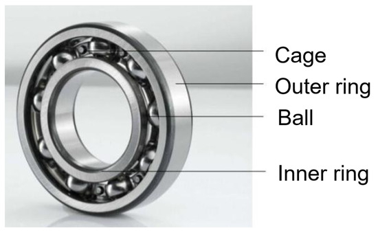
Figure 1.
The basic structure of deep groove ball bearing.
The operating condition of rolling bearings is crucial for the proper functioning of mechanical equipment. With the advancement of smart sensors, the state of bearings can be monitored using data collected from vibration signal sensors. Vibration signals contain a wealth of useful information, and obtaining vibration data through accelerometers is relatively straightforward. During normal operation, the internal components of the bearing remain relatively stable, and the vibration exhibits periodic changes. However, abnormal vibrations can occur due to various reasons during the production or use of bearings. Common forms of bearing vibration include the following:
- Impact Vibration: The rolling elements impact the inner and outer rings during operation, causing radial vibration at the bearing’s natural frequency, with more noticeable vibration on the outer ring.
- Manufacturing Errors: Errors in the manufacturing process can lead to changes in the position or load-bearing state of the rolling elements, causing elastic deformation and vibration. Waviness marks on the rolling elements can also result in abnormal vibrations.
- Poor Lubrication: Insufficient lubrication causes deformation of internal components and changes in the load on the rolling elements, leading to nonlinear vibration signals.
- Wear: Prolonged operation introduces fine particles, causing wear and enlargement of internal clearances, resulting in pulse-type vibration. The speed affects the vibration cycle, and wear increases the vibration amplitude and frequency domain signals.
The performance of rolling bearings gradually declines with use, progressing from normal operation to eventual failure. Understanding the patterns of performance degradation and conducting reliability assessments can help reduce losses from failures and lower equipment costs. The operation of bearings can be divided into four stages: In the healthy state, the equipment is stable and working normally. In early failure, performance begins to degrade. In medium-term failure, there is failure accumulation and performance degradation, so the bearing needs maintenance. In late failure, the damage is serious, the reliability is reduced to 0, and it cannot work normally.
4. Vibration Signal Denoising
4.1. CYCBD
The objective of CYCBD is to extract fault excitations from a noise-contaminated raw signal while filtering out noise components. The specific steps of CYCBD are as follows.
The rolling bearing signal can be represented x, and its transmission and deconvolution process can be expressed using the convolution of a Linear Time-Invariant (LTI) system as follows:
where s represents the result after deconvolution, ⊗ denotes the convolution operation, and h is the Finite Impulse Response (FIR) inverse filter. The above equation can be expressed in matrix form as , as shown below.
The periodicity of the bearing vibration signal can be described as a cyclostationary process [28]. The cyclic frequency, which reflects the periodic fluctuations in signal energy, is defined as follows:
where , N denotes the length of the inverse filter, and T is the rotation period of the shaft.
CYCBD aims to maximize the second-order cyclostationarity indicator () and is solved using an iterative eigenvalue decomposition algorithm. The general expression for second-order cyclostationarity is shown in the equation below:
in the formula, j represents the imaginary unit, the superscript H denotes the conjugate transpose of a matrix, and is the value of the signal s at time l. The matrix E is defined as , and L represents the length of the signal s.
According to the above types, can be re-expressed as:
Let denote the signal containing the periodic components of ; the periodic components of the signal can be expressed as follows:
By substituting the above formula into solution process, we can obtain:
and the weighting matrix W can be expressed as:
In the formula, diag is an operator used to generate diagonal matrices, and and represent the weighted correlation matrix and the correlation matrix, respectively. Solving for the optimal filter is transformed into solving for the maximum eigenvalue and its corresponding eigenvector of .
CYCBD will continue to iterate until the convergence condition is met. When is maximized, the corresponding h is the ideal inverse filter, and the signal obtained after filtering is the noise-reduced signal.
4.2. Ivy Optimization Algorithm
The Ivy optimization algorithm (IVY), proposed by Mojtaba Ghasemi et al. in 2024 [29], is an innovative intelligent optimization algorithm. This algorithm emulates the growth patterns of ivy plants, achieving optimization by orchestrating the orderly population growth and the diffusion and evolution processes of ivy [30,31]. IVY leverages knowledge from neighboring ivy plants to determine growth directions and self-improves by selecting the nearest and most influential neighbors, thereby continuously enhancing solution accuracy. The algorithm principle is as follows:
- Population Initialization:The Ivy algorithm models the population as a group of ivy plants, where each individual represents a potential solution. During initialization, the ivy population can be expressed as , where the i-th population is defined as , . Each individual in the population (i.e., ivy plant) has a randomly generated position, representing the potential solution in the search space. The position is calculated as follows:where is a vector of dimension D with elements uniformly distributed in the range ; and are the lower and upper bounds of the search space, respectively; and ⊙ represents the Hadamard product (element-wise multiplication) between two vectors.
- Coordinated and Ordered Population Growth:This algorithm uses a differential equation to simulate the growth rate of ivy. It considers the relationship between the growth rate and time, and adjusts the growth rate and correction factors and to simulate the ivy’s adaptation to the environment and resource acquisition strategy. The population growth rules are as follows:the vectors and represent the growth rates at time t and , respectively. rand is a random real number within the interval . is a random number with a probability density function equal to . denotes a random vector that follows a normal distribution, where 1 is the mean and is the dimension.
- Path to Sunlight and Growth Strategy:In natural environments, it is crucial for ivy to find a surface to attach to in order to climb toward sunlight. In forests, young ivy typically prioritizes nearby trees as growth targets, which are often already occupied by mature ivy. Through this strategy, ivy gradually expands its coverage, eventually forming a vast, interconnected area across the forest. The young ivy clings to the mature ivy for climbing, and this competitive mechanism ultimately ensures that only the strongest individuals survive within the entire ivy population, regardless of their age.The following equation describes how a young ivy utilizes an older ivy to climb and logically move in the direction of the light source:the absolute value of is the absolute value of , and is the Hadamard division of vector u by vector v.
- The Propagation and Evolution of Ivy Plants:After the young ivy has explored the search space to find its closest and most significant neighbor , it enters a subsequent phase. In this phase, the young ivy endeavors to directly follow the most outstanding member of the entire population, denoted as . This stage can be mathematically formulated as follows:the new growth rate of the current member is calculated by the following formula:
4.3. IVY-CYCBD Algorithm
For a raw vibration signal, the Cyclostationary Blind Deconvolution (CYCBD) algorithm can effectively perform denoising. However, the choice of two key parameters, the cyclic frequency and filter length, has a significant impact on the denoising performance. If the cyclic frequency is set too low, the filter may not sufficiently suppress the noise; while if the cyclic frequency is set too high, it may suppress the useful components of the signal, thereby affecting the denoising effect. Similarly, the selection of filter length is also crucial. A filter that is too short may not effectively capture the signal features, while a filter that is too long may introduce computational complexity, affecting the algorithm’s efficiency.
Therefore, optimizing these two parameters is essential for improving the denoising performance of the CYCBD algorithm. In this section, we focus on optimizing both the cyclic frequency and filter length, and propose a novel IVY-CYCBD algorithm. This algorithm adaptively adjusts these two parameters, achieving efficient denoising of vibration signals. The specific process of the algorithm is shown as follow in Figure 2:
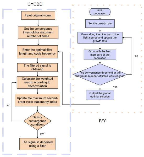
Figure 2.
IVY-CYCBD flow chart.
5. Rolling Bearing Reliability Model
The noise reduction signal processed by the IVY-CYCBD algorithm needs further feature engineering to extract key feature information from it. These features are then processed by dimensionality reduction methods to reduce the dimension and retain the main information, ensuring the validity and operability of the data. Finally, based on the extracted features, the reliability model is applied to evaluate the bearing health state, so as to provide a scientific basis for the bearing fault prediction and life evaluation.
5.1. PaCMAP
Pairwise Controlled Manifold Approximation Projection (PaCMAP) is an efficient and robust nonlinear dimensionality reduction algorithm designed to embed high-dimensional data into low-dimensional space while preserving the geometric and topological characteristics of the data to the greatest extent. At present, it is used by many scholars in the field of data dimensionality reduction [32,33].
By optimizing pairwise distance relationships between data points, the algorithm balances the preservation of local neighborhood structures and global distribution patterns, effectively maintaining data integrity and revealing the intrinsic features.
Compared to other dimensionality reduction methods, PaCMAP demonstrates superior computational speed and the ability to retain global structures, making it particularly suitable for reducing the dimensionality of high-dimensional complex data. The algorithm follows three main steps:
- Construction phase:PaCMAP uses edges to construct the basic structure of a graph. PaCMAP distinguishes three types of edges: neighbor pairs, medium-near pairs, and distant pairs. The first type of edge includes the nearest neighbors of each sample point in high-dimensional space. The following scaled distance metric is used for calculation:where represents the average Euclidean distance from sample point i to its fourth to sixth nearest neighbors. This scaled distance is used to construct neighbor pairs . The scaling process is designed to address the issue of significant differences in neighborhood scales that may occur in different regions of the feature space. Therefore, the scaled distance is used only for the neighbor selection process and not for subsequent optimization stages.The second type of edge includes medium-near pairs randomly selected from each sample, with an additional six observations randomly drawn from each observation value, and the second smallest medium-near pair among them is used.The third type of edge consists of distant pairs randomly selected from the sample each time. The number of medium-near pairs and distant pairs is determined by the parameters and , which specify the ratio of the number of these pairs to the number of nearest neighbors, that is, and .PaCMAP uses three different loss functions for each type of pair:where . The loss function for these edge pairs is determined by the overall loss weighted by , , and .
- Initialization:Although the initialization method has little impact on the results of PaCMAP, Principal Component Analysis (PCA) is still used to reduce actual running time.
- Iterative Optimization:The iterative process is divided into three phases to avoid falling into local optima. In the first phase (from the first iteration to the Nth iteration), the weight of the medium-near pairs is gradually reduced with the goal of improving the initial positions of the embedding points, preserving both global and local structures to some extent. In the second phase (from the Nth iteration to the Mth iteration), the objective is to refine the local structure by assigning a small (non-zero) weight to the medium-near pairs, while maintaining the global structure captured in the first phase. Finally, in the third phase (from the Mth iteration to the end), the focus is on improving the local structure by reducing the weight of the medium-near pairs to zero and decreasing the weight of the neighbor pairs to an even smaller value, emphasizing the role of repulsive forces to help separate potential clusters and make boundaries clearer.
5.2. Logistic Regression Model
Logistic regression is a commonly used method for evaluating the reliability of mechanical equipment. It is employed to predict the probability of an event occurring based on a set of feature parameters. The core of the model consists of linear regression and the Sigmoid function.
The process of a bearing transitioning from normal state to failure is usually divided into a healthy stage and failure stage. Logistic regression can well describe the state transition by mapping the input features to failure probability through the Sigmoid function. Logistic regression assumes that the input characteristics have a linear relationship with the logarithmic probability, while some physical quantities in the process of bearing degradation often have an approximate linear relationship with the failure risk. Its high efficiency, interpretability, and low data requirements make it an ideal choice for engineering practice.
Through the Sigmoid function, logistic regression maps output values to the range of 0 to 1, representing the probability of the event occurring. The Sigmoid function is a monotonically increasing function, and its characteristics are illustrated in Figure 3.
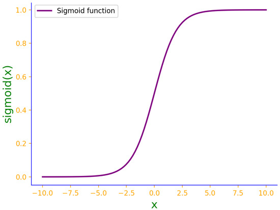
Figure 3.
Sigmoid function.
Assume at time t, the i-th dimensional feature parameter set is , and indicates that the bearing can operate normally at time t. The reliability can be expressed as the logistic function of :
where are the regression coefficients of the feature vector set. The regression coefficients of the logistic regression model are usually estimated using the maximum likelihood estimation method. First, the above equation is transformed:
Let be the set of regression coefficients. Substituting these into the previous equation can obtain
By applying the gradient descent method to solve the above equation, the regression coefficients corresponding to the feature vector set can be obtained. These regression coefficients can then be substituted into the reliability calculation formula to construct a logistic regression reliability evaluation model, enabling the quantitative analysis of bearing reliability.
6. Reliability Prediction Model
Bearing reliability prediction is realized by machine learning model training using dimensionality reduction features. Firstly, the key features are extracted from the original signal by feature engineering, and the redundant information of the features is reduced by the dimensionality reduction method, so as to improve the data processing efficiency. Then, the dimensionally reduced features are input into the model for training. Through the training and optimization of the model, an accurate prediction model can be obtained, which can effectively evaluate the reliability of bearings, make fault predictions, and provide important decision support for the maintenance and management of bearings.
6.1. RVM
The Relevance Vector Machine (RVM), proposed by Tipping in 2001 [23], is a type of sparse probabilistic model. Its fundamental concept is to achieve model sparsity based on the theory of sparse Bayesian learning, integrated with Markov properties, maximum likelihood estimation, and automatic relevance determination (ARD) priors. During the iterative process of the RVM, the posterior distributions of most feature parameters will converge towards zero, indicating that the information contained in these features is redundant for classification. The features with non-zero posterior distributions are referred to as “relevance vectors”, which can reflect the most critical information in the data.
Let and represent the input and output of the training samples, respectively. It can be obtained by the following formula:
In the formula, represents the noise with a mean of zero and variance , is the kernel function, C is the bias, and is the weight vector.
The Relevance Vector Machine (RVM), as an efficient algorithm, is capable of mapping original nonlinear data into a high-dimensional feature space, making the data linearly separable in this new space. This mapping not only significantly simplifies the complexity of the problem but also effectively reduces computational costs.
Due to the complexity of bearing signal data, relying solely on a single kernel function makes it difficult to fully capture its characteristics. To enhance the learning ability of the model, the multi-kernel learning method combines various kernel functions with different characteristics, allowing the model to focus on both global and local features of the data, thereby demonstrating superior performance. When dealing with complex data, multi-kernel functions often outperform single kernel functions. Based on this, this study proposes a weighted combination of polynomial kernel functions with global response characteristics and Gaussian kernel functions with local response characteristics to construct a new mixed kernel function. Combined with this composite kernel function , a Mixed Kernel Relevance Vector Machine (MKRVM) model is designed for bearing performance prediction. Its expression is as follows:
where is the weight parameter used to adjust the influence of different kernel functions; and represent the Gaussian kernel function and the polynomial kernel function, respectively; , b, c, and d are the parameters corresponding to the kernels. This model not only fully utilizes the complementary advantages of the polynomial kernel function and the Gaussian kernel function but also effectively enhances the feature extraction and prediction capabilities for complex bearing signals, providing a new approach for accurate performance evaluation.
6.2. AdaBoost-MKRVM
Adaptive Boosting (AdaBoost) is a classical boosting algorithm used to improve the performance of a model. Its core idea is to improve model accuracy by combining multiple weak learners to form a strong learner. Although MKRVM has powerful feature extraction capabilities, a single MKRVM may still be affected by data noise or local extreme values. In order to further improve the generalization ability of the model, the AdaBoost mechanism was used in this study to integrate multiple MKRVMs to build a stronger learner for reliability prediction of rolling bearings. The following is a detailed description of the AdaBoost-MKRVM algorithm:
- Initialize weights:Suppose the training dataset is , where is the input sample and is the corresponding label. Initialize the weight of the i-th sample, set , meaning all samples have equal weight.
- Iteratively train the MKRVM weak learners:Input the initial feature parameters into the MKRVM to obtain the j-th initial weak learners:Calculate the error of the weak learners :where is the indicator function, which takes the value of 1 when , and 0 otherwise. Adjust the weight coefficient of the j-th sample based on its error:Next, according to the magnitude of the weight coefficients, redistribute the weights of each sample and adjust the sample distribution. The weight of the j-th sample is adjusted to
- Construct the strong learners: The final strong learners is composed of the weighted sum of P weak learners, with the formula
In each iteration, AdaBoost focuses on samples that have been misclassified by the previous round of learners, and by gradually adjusting the sample weights, subsequent learners can better handle samples that are difficult to classify. The algorithm is simple and easy to operate, and has strong generalization ability.
The combination of AdaBoost and MKRVM can give full play to the advantages of both, thus significantly improving the generalization ability and accuracy of the model. AdaBoost improves adaptability and robustness to complex data by integrating multiple weak classifiers, while MKRVM takes advantage of kernel functions to efficiently handle nonlinear problems. After the combination of the two, the model can not only capture data features more comprehensively, effectively reducing the risk of overfitting, but also maintain a high computational efficiency, which is an effective strategy to improve performance. The specific flow chart of the algorithm in Figure 4:
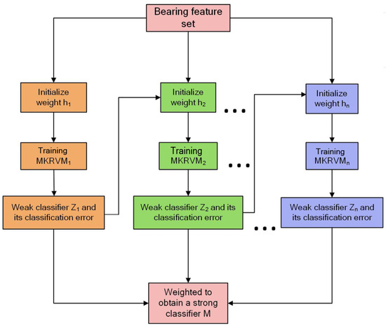
Figure 4.
AdaBoost-MKRVM.
7. Experimental Verification
7.1. Experimental Data Source
In this study, the full life cycle test data of rolling bearings was provided by the Xi’an Jiaotong University-Sunrise Technology Joint Laboratory. The test platform used in the experiment is shown in Figure 5. It mainly consists of an AC motor, a speed controller, and acceleration sensors, with the test bearings being LDK UER204 rolling bearings (The LDK UER204 rolling Bearing is manufactured by LDK Bearing Co., Ltd., Osaka, Japan, and its country of origin is Japan).
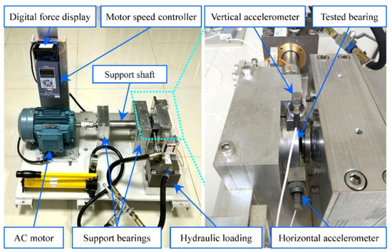
Figure 5.
Test platform.
The experiment employed two PCB 352C33 acceleration sensors, the PCB 352C33 acceleration sensor was manufactured by PCB Piezotronics of Depay, New York (now part of AMETEK Group) and originated in the United States. placed in the horizontal and vertical directions to collect vibration signals of the bearings under three operating conditions. For each operating condition, tests were conducted on five bearings. The sampling frequency was set to 25.6 kHz, with a sampling interval of 1 min and a sampling duration of 1.28 s per instance. The basic parameters of the bearings are provided in Table 1.

Table 1.
Basic parameters of bearings.
7.2. Signal Noise Reduction
To evaluate the noise reduction effectiveness of the LVY-CYCBD algorithm proposed in this paper, we analyze the first set of sampled signals from Bearing 3_1. The time-domain waveform and the envelope spectrum of the vibration signal in the horizontal direction are shown in Figure 6.
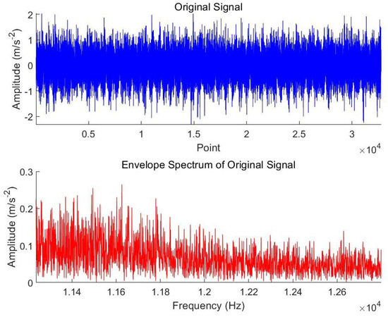
Figure 6.
Bearing 3_1 signals.
From the time-domain waveform, it can be observed that the signal contains significant noise, making it difficult to identify distinct periodic pulse features. In the envelope spectrum, there are numerous interference spectral lines, and the spectrum appears cluttered, indicating a high noise content in the signal.
The proposed LVY-CYCBD algorithm is applied to denoise the signal. Compared with commonly used optimization algorithms, the IVY algorithm demonstrates significant advantages in performance. This study compares it with the Particle Swarm Optimization (PSO) algorithm and the Sparrow Search Algorithm (SSA). Figure 7 illustrates the convergence trends of the three methods. As shown in the figure, the IVY algorithm achieves the optimal fitness value in the fourth iteration. Compared with the other two algorithms, the IVY algorithm not only converges the fastest but also achieves the highest convergence accuracy.
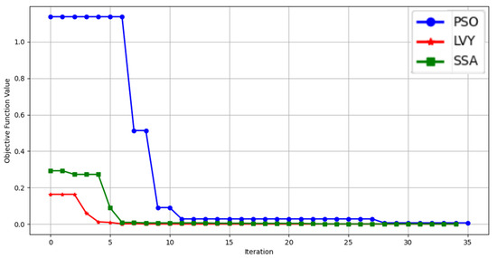
Figure 7.
Convergence trend diagram.
In this study, the LVY optimization algorithm was used to optimize two key parameters in the CYCBD method: cyclic frequency and filter length. Through experiments, the optimal cyclic frequency was determined to be 114 Hz, and the optimal filter length was 85. These parameters were adopted as the final LVY-CYCBD algorithm settings. The LVY-CYCBD algorithm was compared with the CYCBD algorithm without parameter optimization (cyclic frequency of 90 Hz and filter length of 100). The time-domain waveform and envelope spectrum obtained from processing the experimental signals are shown in the Figure 8 and Figure 9.
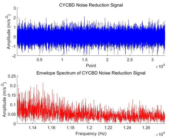
Figure 8.
Signal after CYCBD processing.
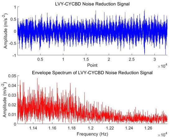
Figure 9.
Signal after LVY-CYCBD processing.
As shown in the figure, compared to the original method, both the LVY-CYCBD algorithm and the traditional CYCBD algorithm effectively suppress noise interference in the signal, making the periodic pulse components more prominent. Additionally, a comparison of the envelope spectrums of the two methods reveals that the peak value of the envelope spectrum after denoising with the LVY-CYCBD algorithm does not exceed 0.00005 m/s2, which is significantly lower than that of the unoptimized CYCBD algorithm. In terms of both noise amplitude and peak amplitude characteristics, the LVY-CYCBD algorithm demonstrates substantial improvement. This indicates that the LVY-CYCBD algorithm effectively reduces signal noise, enabling the extracted bearing characteristic frequencies to become clearer and more informative.
To more intuitively evaluate the performance of denoised and reconstructed signals, this study compares the denoising effectiveness of the CYCBD, LVY-CYCBD, and CEEMDAN algorithms using the signal-to-noise ratio (SNR) metric. The specific results are shown in Table 2. The results indicate that the LVY-CYCBD algorithm achieves a notable improvement in SNR compared to the other algorithms.
Table 2.
Comparison of model noise reduction effect.
7.3. Signal Feature Extraction
Although most of the noise has been removed, the denoised vibration signal still cannot directly reflect the trend of bearing performance changes. However, vibration signals are rich in data features and easy to extract, making feature extraction an indispensable step in bearing trend prediction. Based on the needs of reliability prediction, this study uses three methods—time-domain, frequency-domain, and time–frequency-domain—to extract features.
This study referred to a lot of literature [21] and selected 12-dimensional features on the basis of experiments. Through the operation of calculating Pearson correlation coefficient of all feature pairs (threshold value is 0.85), some features in the literature [21] were deleted. The 12-dimensional features are selected, which have been widely studied and applied in related fields, and are considered to be able to better reflect the characteristics of signals or data. At the same time, considering the computing resources and data processing efficiency in practical applications, selecting the right amount of features helps to avoid excessive computing costs and data dimension disasters. These 12 features can not only guarantee the prediction performance, but also reduce the computational complexity and make the model more operable.
Regarding feature composition, time-domain features (standard deviation, kurtosis, rectified mean, skewness, peak value, and impulse factor) directly reflect amplitude variations in vibration signals and can effectively capture impact events caused by bearing surface damage (e.g., spalling and cracks); frequency-domain features (spectral skewness, mean square frequency, dominant frequency, and spectral entropy), extracted through Fourier transform, can more effectively characterize signal periodicity, vibration modes, and energy distribution; and time–frequency-domain features (instantaneous frequency and singular value entropy) combine temporal and spectral information, making them suitable for non-stationary signal analysis and capable of capturing time-varying characteristics of fault features. This feature selection approach significantly reduces feature dimensionality while maintaining diagnostic performance.
Figure 10 shows the 12-dimensional feature parameter set extracted from bearing 3-1.
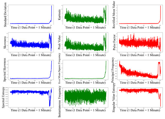
Figure 10.
The 12-dimensional feature parameter set.
The feature parameter initial selection set, composed of the 12 time-domain, frequency-domain, and time–frequency-domain features mentioned above, can more comprehensively reflect the changing trends in the bearing’s operating condition.
7.4. Bearing Reliability Modeling
The initial feature parameter set consists of high-dimensional feature vectors, which can be challenging to directly incorporate into reliability models for solving reliability problems, potentially even leading to the curse of dimensionality. In this study, the PacMAP algorithm is employed to perform dimensionality reduction on the degradation feature parameter set. Based on the characteristics of bearing degradation data, 2D is selected as the target dimensionality for reduction. This choice not only better preserves both local and global structures of the data but also provides more intuitive spatial visualization effects.
Figure 11 illustrates the relationship between the dimensionality reduction levels (from 1D to 5D) and both the variance retained and relative computation time. The left vertical axis represents the variance retained, while the right vertical axis shows the relative computation time. Through cumulative variance contribution rate analysis, it was found that 2D reduction retains approximately 91.24% of the original information, 3D retains about 92.31%, 4D retains around 93.43%, and 5D retains approximately 93.67%. As shown in the figure, the computation time increases nonlinearly with higher dimensions (5D requires about 2.5 times the computation time of 2D). Selecting higher dimensions does not significantly improve the variance contribution rate but substantially increases computational complexity. Therefore, this study opts to reduce the data to two dimensions.
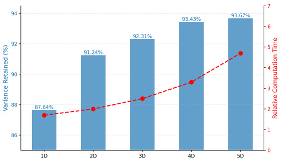
Figure 11.
Variance retention rate and computation time vary with dimension.
Additionally, T-Distributed Stochastic Neighbor Embedding (t-SNE) and Principal Component Analysis (PCA) are also used to perform dimensionality reduction on the data. The dimensionality reduction results of the three algorithms are shown in Figure 12.
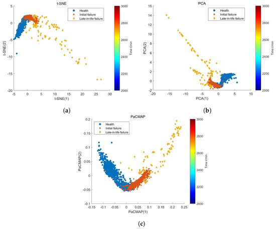
Figure 12.
Dimensionality reduction results of the three algorithms. (a) t-SNE; (b) PCA; (c) PaCMAP.
As shown in the figure, the dimensionality reduction results of t-SNE, PCA, and PaCMAP all exhibit a certain degree of overlap, with data points from different stages crossing over significantly, making it less effective in distinguishing the operational cycles of the bearings. In contrast, the PaCMAP algorithm performs better in segmenting the operational cycles of the bearings. Its dimensionality reduction results more clearly illustrate the separations between the three cycles, with the data points from each stage being more distinctly separated. This indicates that the dimensionality reduction results of the PaCMAP algorithm are more effective in reflecting the degradation conditions of the bearings.
Based on the bearing 3-1 degradation feature set obtained after dimensionality reduction, a model for reliability assessment can be constructed. This study employs an intuitive logistic regression model for the reliability assessment of the bearing. By selecting the three-dimensional feature vector set obtained after dimensionality reduction by PaCMAP as the degradation feature information, and using it as the input for the logistic regression model, the regression coefficients of the logistic regression model are calculated as follows: , , and . These coefficients are then substituted into the logistic regression model’s reliability calculation formula to establish the bearing reliability assessment model:
Based on the aforementioned model, we can generate the actual reliability curve for bearing 3-1. Given that bearing 3-1 functions quite reliably during the initial 2000 min of operation, to more closely examine the timing and severity of any operational failures, we have extracted a segment of the curve representing the first 400 min of the bearing’s operation, as depicted in Figure 13. This focused analysis allows for a more detailed observation of the bearing’s performance and the onset of any potential issues.
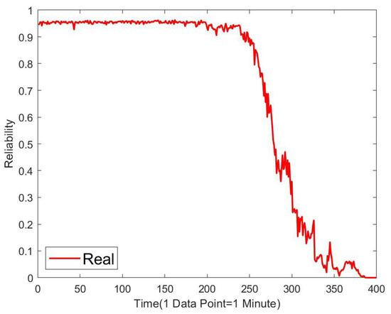
Figure 13.
Bearing 3-1 reliability.
As operating time increases, the reliability of the bearing begins to decline gradually from a value close to 1. In the initial phase of the bearing’s operation, the reliability changes smoothly, which indicates that the bearing is functioning well without any failures. However, at around 2380 min of operation, the reliability curve experiences a drastic change, signaling that the bearing has encountered a failure. After about 2380 min of continuous operation, the reliability curve exhibits significant fluctuations, suggesting that the failure has affected the bearing’s performance and that there may be multiple areas of failure within the bearing. Over time, the bearing’s reliability continues to decrease, implying that its remaining lifespan is progressively reducing until the reliability eventually drops to zero, rendering the bearing completely non-functional. Thus, by establishing a reliability model for the bearing and observing its reliability curve, one can effectively characterize the trend of changes throughout the bearing’s entire life cycle, thereby analyzing the bearing’s operational status.
7.5. Bearing Reliability Prediction
In response to the issue of reliability prediction for rolling bearings, this study proposes a reliability prediction model that integrates AdaBoost ensemble learning and Mixed Kernel Relevance Vector Machine (MKRVM) algorithms. In order to verify the effectiveness of this method, bearings 3-1, 3-2, and 3-4 in the XJTU-SY rolling bearing dataset and bearing 5 in the bearing vibration data from the University of Cincinnati were selected for reliability prediction experiments.
Taking bearing 3-1 as an example, the feature sample set of bearing 3-1 after noise reduction is first extracted, and 12 initial feature parameter sets consisting of features in the time domain, frequency domain, and time–frequency domain are obtained. Dimensionality reduction is then performed using the PaCMAP algorithm, and the resulting three-dimensional feature vector set after PaCMAP dimensionality reduction is selected as the degradation feature information. Bearing 3-1 recorded a total of 2496 time points of data, with the first 2138 samples used for model training and the remaining 400 samples serving as the test set.
Through multiple grid searches to determine the mixed kernel function coefficient (as shown in the first subplot of Figure 14), it was found that when the coefficient is set to 0.73, the model achieves the lowest test error (MAE) of 0.029, along with optimal error stability. Further experiments revealed that when the coefficient fluctuates within the range of 0.7 to 0.75, the variation in MAE remains below 0.005, indicating low sensitivity of the model performance to this parameter and strong robustness.Simultaneously, when the number of base learners reaches 10, the test error stabilizes (as shown in the second subplot of Figure 14). Additional experiments demonstrated that increasing the number of base learners (e.g., to 15 or 20) improves the MAE by less than 0.002 but significantly increases computational costs. Therefore, selecting 10 base learners achieves an optimal balance between performance and efficiency.
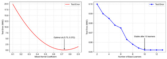
Figure 14.
Test results.
Based on these findings, the mixed kernel function coefficient is ultimately set to 0.73, and the AdaBoost algorithm is configured with 10 base learners. After determining these parameters, the training data are used to predict the bearing’s reliability. The prediction results from the AdaBoost-MKRVM model are then input into a logistic regression model to calculate the regression coefficients, thereby determining the operational reliability of bearing 3-1.
Furthermore, the effectiveness of this prediction method is validated using data from bearings 3-2 and 3-4, with the relevant results presented in Figure 15.
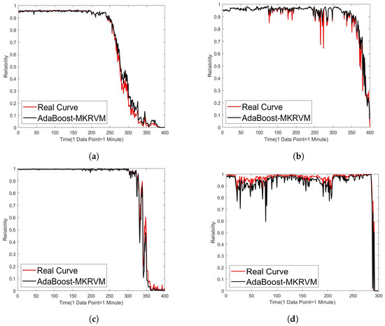
Figure 15.
Four bearing reliability prediction results. (a) Bearing 3-1; (b) bearing 3-2; (c) bearing 3-4; (d) bearing 5.
The reliability curve of bearing 3-1 is shown in Figure 15a. It can be observed that bearing 3-1 operated relatively stably in the early stages, but a serious failure occurred in the last 150 points of operation, resulting in a rapid decline in reliability. Figure 15b shows the reliability curve of bearing 3-2. During operation, the reliability continues to fluctuate slightly, indicating that faults gradually accumulate and eventually lead to faults. Figure 15c shows the reliability curve of bearing 3-4, where the reliability remains relatively stable until the last 300 points, and then drops sharply to zero during the last 100 points. Figure 15d shows the reliability curve of bearing 5 of the University of Cincinnati. Due to the small number of sample points of this bearing, the last 300 samples were selected as the test set. It can be seen in the figure that the bearing began to completely fail at the last 20–30 sample points. Comprehensive analysis shows that the predicted reliability values of the four kinds of bearings are in good agreement with the actual reliability trend, which indicates that the proposed method can accurately predict the bearing reliability change.
To validate the predictive accuracy of the AdaBoost-MKRVM model, this study employed Long Short-Term Memory (LSTM), Bidirectional Long Short-Term Memory (Bi-LSTM), Gated Recurrent Unit (GRU), Least Squares Support Vector Machine (LSSVM), and MKRVM models to predict the reliability of bearings 3-1, 3-2, 3-4, and 5. The results were compared with those of the AdaBoost-MKRVM model. In the LSTM neural network, the number of neural network layers is set to 3; the neuron excitation function is set to Sigmoid function; and the number of input neurons of each layer, the hidden layer, and the output layer are set to 10 layers, 14 layers, and 1 layer, respectively. The GRU settings are the same as LSTM. In LSSVM, the Gaussian kernel function is used, and the penalty factor and kernel function parameters are set to 9, 0.002. In RVM, the Gaussian kernel function is used, and the penalty factor and kernel parameter are set to 9, 0.002. In MKRVM, the Gaussian kernel function and linear kernel function are used. The penalty factor and kernel argument are set to values of 9, 0.002. The mean absolute error (MAE) and mean absolute percentage error (MAPE) for each prediction model are presented in Table 3. The results of the last two AdaBoost-MKRVM training and test sets show that the error gap is very small, indicating that the model has good generalization ability and can maintain a similar performance on new data as in the training.
Table 3.
Prediction accuracy comparison of different models.
From Figure 15, it can be seen that compared to existing bearing reliability prediction methods, the MKRVM model provides a prediction curve that is closer to the actual reliability curve, with smaller prediction errors. According to the error values of various bearing prediction methods shown in Table 3, representing them in the form of a bar chart as in Figure 16 allows for a more intuitive comparison, clearly demonstrating that the prediction error values obtained by the MKRVM model are smaller than those of other prediction methods.
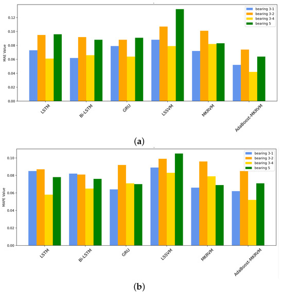
Figure 16.
Four bearing reliability prediction results. (a) MAE; (b) MAPE.
This study addresses the issue of reliability prediction for rolling bearings, starting with vibration signals. An improved CYCBD algorithm based on the Ivy optimization algorithm was proposed to efficiently remove signal noise. A reliability modeling method based on logistic regression was developed, and an ensemble learning model combining AdaBoost and MKRVM was further applied for precise reliability prediction of the bearings, demonstrating the effectiveness and accuracy of the proposed approach.
8. Conclusions
Aiming at the problem of reliability prediction of rolling bearings, this study proposed CYCBD algorithm improved by Ivy optimization algorithm to efficiently remove signal noise from vibration signals. The reliability modeling method based on logistic regression is constructed, the integrated learning model combining AdaBoost and MKRVM is further used to accurately predict the bearing reliability, and the effectiveness and accuracy of the method are verified. The innovations of this paper are as follows:
- Improved Denoising Method: A CYCBD method enhanced by the Ivy algorithm is proposed for efficiently denoising bearing vibration signals. By optimizing the cyclic frequency and filter length of the CYCBD method using the Ivy algorithm, noise components in the signal are effectively removed, significantly improving the denoising performance.
- Feature Dimensionality Reduction and Visualization: To address the issue of high-dimensional bearing feature sets, a novel dimensionality reduction method, PaCMAP, is employed. This method reduces the dimensionality of multidimensional feature sets and achieves visualization of the feature space, providing a more intuitive analysis of feature distributions.
- Reliability Prediction Model: To meet the reliability prediction requirements of rolling bearings, an AdaBoost-MKRVM-based prediction model is developed. This model integrates ensemble learning with the Relevance Vector Machine to improve prediction accuracy, offering an effective solution for rolling bearing reliability evaluation.
Compared with the results of the citation [23] with similar logic, the prediction error RMSE is 0.8982, and the MAE of the AdaBoost-MKRVM prediction model proposed in this paper is 0.052, which further improves the prediction accuracy.
9. Discussion
This study focuses on the reliability evaluation and prediction of rolling bearings, and the effectiveness of the proposed methods has been validated through experimental data. However, several issues remain to be addressed. Future research can explore the following directions:
- Signal Denoising Methods: This study improved the denoising performance by enhancing the CYCBD algorithm. Experimental results show that the improved CYCBD algorithm outperforms traditional methods (such as wavelet transform and EMD) in noise suppression and fault feature extraction. Future research can develop more targeted and adaptive denoising methods based on the characteristics of bearing signals to further improve the efficiency and effectiveness of noise reduction. For example, deep learning techniques can be integrated to design end-to-end denoising models.
- Adaptability to Complex Operating Conditions: The validation data in this study were primarily obtained from laboratory equipment under ideal experimental conditions and relatively stable operating environments. However, actual operating conditions are often complex and variable, especially under varying speed and load conditions, which require further investigation. Future work can explore data collection and model training methods under multiple operating conditions to enhance the applicability and robustness of the methods in real-world industrial environments.
- Model Optimization and Extension: Although the AdaBoost-MKRVM model demonstrated high prediction accuracy in this study, its computational complexity may limit its application in real-time systems. Future research can investigate more efficient model optimization methods, such as hardware-accelerated computing or model compression techniques. Additionally, other machine learning models (e.g., deep learning or reinforcement learning) can be explored for bearing reliability prediction.
- Multi-Sensor Data Fusion: The current study primarily analyzes vibration signals. Future research can integrate multi-sensor data (e.g., temperature, acoustic signals) for fusion analysis to improve the accuracy of fault diagnosis and reliability prediction. Multi-source data fusion can provide a more comprehensive reflection of the bearing’s operating state, offering more reliable support for the health monitoring of industrial equipment.
Future research should focus on these directions to refine existing approaches and advance the practical application of reliability evaluation and prediction technologies for rolling bearings.
Author Contributions
Y.Y. wrote the manuscript; Y.Y. and S.C. performed the experiment and simulation; Y.Y. and D.G. processed the experimental data and participated in the revision of the manuscript; J.Q. provided financial support. All authors have read and agreed to the published version of the manuscript.
Funding
This research was supported by the Nantong Institute of Technology electronic information master’s project (879002), National College Computer Basic Education Teaching Research Project (2024-AFCEC-088), Nantong Institute of Technology University-level “Public Course Education Teaching Reform Research” project (2024JGG015).
Data Availability Statement
All data generated or analyzed to support the findings of this study are included within the article.
Conflicts of Interest
The authors declare no conflicts of interest.
References
- Gao, L.; Gu, Y.; Chen, C.; Zhang, P.; Zhang, Z. Wind Turbine Gearbox Bearing Fault Diagnosis Method Based on ICEEMDAN and Flexible Wavelet Threshold. J. Fail. Anal. Prev. 2024, 24, 1181–1198. [Google Scholar]
- He, F.; Ye, Q. A Bearing Fault Diagnosis Method Based on Wavelet Packet Transform and Convolutional Neural Network Optimized by Simulated Annealing Algorithm. Sensors 2022, 22, 1410. [Google Scholar] [CrossRef] [PubMed]
- Liu, Y.; Kang, J.; Bai, Y.; Guo, C. Research on the health status evaluation method of rolling bearing based on EMD-GA-BP. Qual. Reliab. Eng. Int. 2023, 39, 2069–2080. [Google Scholar]
- Wiggins, R.A. Minimum entropy deconvolution. Geoexploration 1978, 16, 21–35. [Google Scholar]
- McDonald, G.L.; Zhao, Q.; Zuo, M.J. Maximum correlated Kurtosis deconvolution and application on gear tooth chip fault detection. Mech. Syst. Signal Process. 2012, 33, 237–255. [Google Scholar]
- Sun, Y.; Yu, J. Fault feature extraction of rolling bearings using local mean decomposition-based enhanced sparse coding shrinkage. J. King Saud Univ. 2022, 34, 17–22. [Google Scholar]
- Liu, P.; Lin, Z.; Zhang, M.; Gu, Y. Fault Diagnosis of Rolling Bearing based on Permutation Entropy Optimized Maximum Correlation Kurtosis Deconvolution. IOP Conf. Ser. Mater. Sci. Eng. 2021, 1043, 022029. [Google Scholar]
- Buzzoni, M.A.J.G. Blind deconvolution based on cyclostationarity maximization and its application to fault identification. J. Sound Vib. 2018, 432, 569–601. [Google Scholar]
- Miao, Y.; Shi, H.; Lin, H.J. Period-refined CYCBD using time synchronous averaging for the feature extraction of bearing fault under heavy noise. Struct. Health Monit. 2024, 23, 1071–1088. [Google Scholar]
- Huo, W.; Jiang, Z.; Sheng, Z.; Zhang, K.; Xu, Y. Cyclostationarity blind deconvolution via eigenvector screening and its applications to the condition monitoring of rotating machinery. Mech. Syst. Signal Process. 2025, 222, 111782. [Google Scholar]
- Wang, Z.; Zhou, J.; Du, W.; Lei, Y.; Wang, J. Bearing fault diagnosis method based on adaptive maximum cyclostationarity blind deconvolution. Mech. Syst. Signal Process. 2022, 162, 108018. [Google Scholar]
- Zhang, Q.; Pan, H.; Fan, Q.; Xu, F.; Wu, Y. Research on Fault Extraction Method of CYCBD Based on Seagull Optimization Algorithm. Shock Vib. 2021, 13, 1–11. [Google Scholar]
- Maierhofer, J.; Gänser, H.P.; Daves, W.; Eck, S. Digitalization and Reliability of Railway Vehicles and Tracks—Condition Monitoring and Condition-based Maintenance. BHM Berg-Hüttenmänn. Monatshefte 2024, 169, 264–268. [Google Scholar]
- Zhou, F.; Wang, Y.; Jiang, S. Research on an early warning method for bearing health diagnosis based on EEMD-PCA-ANFIS. Electr. Eng. 2023, 105, 2493–2507. [Google Scholar]
- Li, Q.; Yan, C.; Chen, G.; Wang, H.; Li, H.; Wu, L. Remaining Useful Life prediction of rolling bearings based on risk assessment and degradation state coefficient. ISA Trans. 2022, 129, 413–428. [Google Scholar]
- Ye, J.; Xiong, T.; Li, Q.; Janardan, R.; Bi, J.; Cherkassky, V.; Kambhamettu, C. Efficient model selection for regularized linear discriminant analysis. In Proceedings of the 15th ACM International Conference on Information and Knowledge Management, Arlington, VA, USA, 6–11 November 2006; pp. 532–539. [Google Scholar]
- Hinton, G.; Roweis, S. Stochastic Neighbor Embedding. Adv. Neural Inf. Process. Syst. 2003, 15, 833–840. [Google Scholar]
- Mcinnes, L.; Healy, J. UMAP: Uniform Manifold Approximation and Projection for Dimension Reduction. J. Open Source Softw. 2018, 3, 861. [Google Scholar]
- Amid, E.; Warmuth, M.K. TriMap: Large-scale Dimensionality Reduction Using Triplets. arXiv 2019, arXiv:1910.00204. [Google Scholar]
- Wang, Y.; Huang, H.; Rudin, C.; Shaposhnik, Y. Understanding How Dimension Reduction Tools Work: An Empirical Approach to Deciphering t-SNE, UMAP, TriMap, and PaCMAP for Data Visualization. arXiv 2021, arXiv:2012.04456. [Google Scholar]
- Cramer, J.S. The Origins of Logistic Regression; No. 02-119/4; Tinbergen Institute: Amsterdam, The Netherlands, 2002. [Google Scholar]
- Gao, S.; Zhang, S.; Zhang, Y.; Gao, Y. Operational Reliability Evaluation and Prediction of Rolling Bearing Based on Isometric mapping and NoCuSa-LSSVM. Reliab. Eng. Syst. Saf. 2020, 201, 106968. [Google Scholar]
- Tipping, M.E. Sparse Bayesian Learning and the Relevance Vector Machine. J. Mach. Learn. Res. 2001, 1, 211–244. [Google Scholar]
- Cortes, C.; Vapnik, V. Support-Vector Networks. Mach. Learn. 1995, 20, 273–297. [Google Scholar]
- Tang, J.; Zheng, G.; He, D.; Ding, X.; Huang, W.; Shao, Y.; Wang, L. Rolling bearing remaining useful life prediction via weight tracking relevance vector machine. Meas. Sci. Technol. 2021, 32, 024006. [Google Scholar]
- Zhang, G.; Liang, W.; She, B.; Tian, F. Rotating Machinery Remaining Useful Life Prediction Scheme Using Deep-Learning-Based Health Indicator and a New RVM. Shock Vib. 2021, 2021, 8815241. [Google Scholar]
- Wang, Y.; Guo, R.; Liu, G. Remaining Useful Life Prognostics for the Rolling Bearing Based on a Hybrid Data-Driven Method. In Proceedings of the 2020 3rd International Conference on Intelligent Robotic and Control Engineering (IRCE), Oxford, UK, 10–12 August 2020. [Google Scholar]
- Raad, A.; Antoni, J.; Sidahmed, M. Indicators of cyclostationarity: Theory and application to gear fault monitoring. Mech. Syst. Signal Process. 2008, 22, 574–587. [Google Scholar]
- Ghasemi, M.; Zare, M.; Trojovský, P.; Rao, R.V.; Trojovská, E.; Kandasamy, V. Optimization based on the smart behavior of plants with its engineering applications: Ivy algorithm. Knowl. Based Syst. 2024, 295, 111850. [Google Scholar]
- Xiao, P. Research on Fault Diagnosis of Ship Diesel Generator System Based on IVY-RF. Energies 2024, 17, 5799. [Google Scholar] [CrossRef]
- Gao, H.; Wang, H.; Shen, H.; Xing, S.; Yang, Y.; Wang, Y.; Liu, W.; Yu, L.; Ali, M.; Khan, I.A. Multi-modal denoised data-driven milling chatter detection using an optimized hybrid neural network architecture. Sci. Rep. 2025, 15, 3953. [Google Scholar]
- Yousuff, M.; Babu, R.; Rathinam, A. Nonlinear dimensionality reduction based visualization of single-cell RNA sequencing data. J. Anal. Sci. Technol. 2024, 15, 1. [Google Scholar]
- Seghers, E.E.; Briceno-Mena, L.A.; Romagnoli, J.A. Unsupervised learning: Local and global structure preservation in industrial data. Comput. Chem. Eng. 2023, 178, 14. [Google Scholar]
Disclaimer/Publisher’s Note: The statements, opinions and data contained in all publications are solely those of the individual author(s) and contributor(s) and not of MDPI and/or the editor(s). MDPI and/or the editor(s) disclaim responsibility for any injury to people or property resulting from any ideas, methods, instructions or products referred to in the content. |
© 2025 by the authors. Licensee MDPI, Basel, Switzerland. This article is an open access article distributed under the terms and conditions of the Creative Commons Attribution (CC BY) license (https://creativecommons.org/licenses/by/4.0/).