Utilizing Cell Transmission Models to Alleviate Accident-Induced Traffic Congestion in Two-Way Grid Networks

Abstract

The Cell Transmission Model (CTM) is a commonly used framework and cost-effective approach for evaluating transportation-related solutions, particularly for analyzing urban traffic congestion, due to its strong mathematical framework. Its effectiveness relies heavily on accuracy, making proper calibration essential for deriving reliable design decisions. This study utilizes CTM calibration techniques to design control strategies for mitigating accident-induced traffic congestion in two-way grid networks. By modifying the number of downstream cells and their vehicle capacity, we assess the impact of these adjustments on traffic flow efficiency within the grid structure. Additionally, we utilize MATLAB R2022a to design an intelligent transportation network simulation environment, providing a robust platform for testing and optimizing traffic management strategies specific to two-way grid networks. The findings of this research contribute to the introduction of a novel refinement to the traditional CTM by dividing only cell 9 into three smaller cells to accurately capture different movement directions, enhancing intersection modeling without increasing overall computational complexity.

1. Introduction

Traffic congestion in urban networks has increased significantly, becoming a major challenge in many large cities due to the rising number of vehicles. It is marked by slower speeds, longer travel times, and increased vehicle queueing. Congestion occurs when traffic demand exceeds road capacity, causing vehicle interactions to disrupt smooth traffic flow. This article focuses on analyzing and addressing vehicle congestion in urban traffic networks. An intelligent transportation system (ITS) is essential for improving the effectiveness and security of transport networks [1]. The concept of the ITS emerged nearly thirty years ago as part of efforts to address long-term traffic congestion. ITS technologies have been extensively utilized to address traffic congestion challenges, encompassing aspects such as accident detection and validation [2,3,4], emergency response coordination [5], accident-related wireless communications [6], and freeway traffic simulation [7]. Traffic congestion is a complex factor that influences various aspects of traffic accidents. Wang et al. [8] suggested that if the correlation between congestion and fatal or serious injury accidents is negative, congestion may, in some cases, contribute to improved road safety. This poses a challenge for traffic management, as reducing congestion does not always lead to fewer accidents. To address this issue, it is crucial to lower accident rates while gaining a deeper understanding of how congestion impacts traffic incidents. Despite extensive research on the relationship between congestion and accidents, no clear consensus has been reached. Traffic accidents not only cause congestion but also contribute to its spread across urban networks. Therefore, studying the formation and propagation of traffic congestion is essential for developing effective traffic management strategies. Traffic congestion can arise from one of three primary causes [9]: temporary obstructions, permanent capacity constraints, or stochastic fluctuations in demand. Accidents are a type of temporary obstruction, often leading to congestion. In this research, we concentrate on traffic congestion resulting from accidents within two-way grid networks. Qi et al. [10] classified accident-induced congestion as a distinct type of traffic jam, emphasizing that if accidents are not cleared promptly, they can trigger large-scale upstream congestion.

In recent years, considerable research has been dedicated to understanding accident-induced traffic jams, leading to the development of both analytical models [11] and accident simulation models that examine congestion formation and growth [12]. Additionally, Roberg et al. [13] classified traffic control strategies for accidents into static and dynamic methods. Static strategies emphasize roadway design elements to minimize congestion spread, whereas dynamic approaches focus on real-time interventions to control and alleviate congestion propagation. By integrating these strategies, traffic management systems can more effectively address congestion resulting from accidents. Moreover, various methodologies [13,14,15,16,17,18,19,20,21,22,23,24,25,26,27,28,29] have been proposed to mitigate traffic congestion. Nevertheless, the majority of existing control strategies prove most effective under low-to-moderate traffic flow and stable conditions, restricting their suitability for more intricate and dynamic traffic environments. To alleviate urban traffic congestion caused by accidents, various rerouting strategies have been implemented with the support of traffic authorities. Notably, several studies [14,15,16,17] focus on dispersing incident-induced traffic jams in urban networks. Typically, red lights are used to prevent vehicles from entering congested areas [17,18,19,20]. Long et al. [14] introduced a diamond control strategy that prevents all vehicles from entering a specifically designated diamond-shaped area. Qi et al. [10] introduced a strategy that combines banning and warning signals to mitigate accident-induced congestion. However, a key limitation of this approach is that warning signals alone do not ensure high compliance among drivers. Lou et al. [17] addressed this issue by applying only the ban signal in conjunction with the CTM to analyze traffic congestion. Moreover, a variety of methodologies [21,22,23,24,25,26,27,28] have been proposed to reduce traffic flow.

A review of previous studies suggests that the CTM is well-suited for simulating the formation and dissipation of traffic jams in city transportation systems. However, based on the contributions of CTM-related research [16,17,27,28], two unreasonable phenomena have been identified. In this study, we aim to refine the CTM by adjusting key parameters, including the number of downstream cells and their vehicle capacity, to address these issues. Our study primarily follows the conventional CTM approach by dividing each link into nine cells. However, we refine the model by further dividing only cell 9 into three smaller cells, each representing a distinct movement direction (e.g., left-turn, though, and right-turn). This adjustment allows for a more accurate representation of traffic dynamics at intersections while maintaining consistency with the standard nine-cell structure elsewhere in the network. The choice ensures a balance between computational efficiency and the ability to capture critical congestion patterns at intersections. This study examines the utilization of the CTM in traffic control strategies aimed at dispersing congestion caused by accidents and assesses their effectiveness compared to existing methods.

The rest of this paper is structured as follows: Section 2 succinctly defines the CTM. Section 3 identifies challenges associated with the conventional CTM approach. Section 4 details the simulation of traffic congestion propagation and dissipation within an 8 × 8 two-way grid traffic network. Finally, Section 5 presents the conclusions of this study.

2. Summary of the Cell Transmission Model

It is well known that the CTM is a macroscopic traffic flow model proposed by Daganzo [29]. As far as we know, Daganzo [29,30] first introduced the CTM as an improvement to the Lighthill–Whitham–Richards model [31,32,33]. It is widely used in traffic management due to its strong mathematical framework, which allows for the efficient simulation of traffic dynamics. The CTM divides a road segment into several cells, numbering them as i = 1, 2… n starting from the upstream end, where each cell represents a portion of the roadway with uniform traffic characteristics. The flow of vehicles between cells follows predefined traffic flow principles based on vehicle conservation and the fundamental diagram of traffic flow.

In this article, for simplicity, we consider a two-way grid network G = (C, A) to illustrate simulation results based on our traffic congestion control strategies, adapted from our previous work [17]. In this model, C represents the set of nodes, and A denotes the set of links. 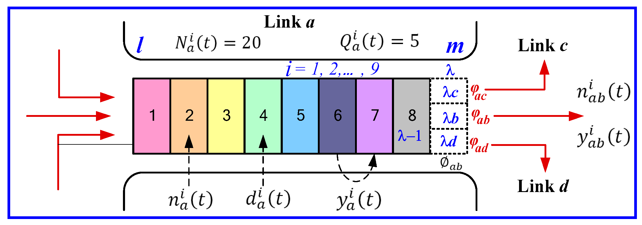A link a = (l, m) connects nodes l and m, where A_l represents the set of links directed toward node l and B_m refers to the set of links departing from node m. Each link is divided into λ discrete cells, with time segmented into intervals such that the length of a cell corresponds to the distance traveled by free-flow traffic within one time interval δ. As shown in Figure 1, each link a consists of two distinct sections [16]: (1) a downstream queue storage area, where vehicles are sorted based on their turning movements, and (2) an upstream reservoir, where turning movements mix. In a specific case, such as the ninth cell, the downstream queue storage area is subdivided into three sections, i.e., φ_ac, φ_ab, and φ_ad, which serve as separate queuing zones.

Table 1. Definitions and corresponding meanings of notations.

Notations	Meaning
${n^i}_a\left(t\right)$	The count of vehicles present in cell i of link a at the beginning of time interval t.
${y^i}_a\left(t\right)$	The quantity of vehicles entering cell i of link a during time interval t.
${N^i}_a\left(t\right)$	The highest possible number of vehicles that can occupy cell i of link a during time interval t.
${Q^i}_a\left(t\right)$	The greatest possible number of vehicles that can enter cell i of link a during time interval t.
${n^i}_{ab}\left(t\right)$	The count of vehicles present in cell i of link a at the beginning of time interval t that have link b as their next destination.
${y^i}_{ab}\left(t\right)$	The quantity of vehicles entering cell i of link a during time interval t that will proceed to link b next.
${d^i}_a\left(t\right)$	The total congestion delay experienced by vehicles present in cell i of link a during time interval t.
${\mathit{\varphi }}_{\mathit{a}\mathit{x}}$	The percentage of vehicles moving from link a to links b, c, and d.
d(t)	The overall congestion delay experienced by all vehicles within the entire network during time interval t.

outlines the key notations, primarily sourced from Luo et al. [17].

Below, we briefly introduce its key parameters and mathematical formulas.

The key parameters in the CTM are as follows:

• Cell Capacity (N_i)—The maximum number of vehicles a cell can hold.
• Free Flow Speed (v_f)—The speed at which vehicles move in uncongested conditions.
• Jam Density (λ)—The maximum vehicle density a cell can sustain before complete congestion occurs.
• Flow Rate (q_i)—The number of vehicles moving from one cell to the next per time step.

The CTM follows two main equations, as follows:

• Conservation Equation:

N_i(t + 1) = N_i(t) + inflow_i−1(t) − outflow_i(t)

where N_i(t) is the number of vehicles in cell i at time t.

2.

Flow Calculation:

q_i(t) = min(d_i(t), s_i+1(t))

where d_i(t) is the demand (vehicles willing to leave the cell) and s_i+1(t) is the supply (available space in the next cell).

For more details, please refer to our previous studies [17,34].

3. Problem Statement

Traffic congestion is a critical challenge in urban transportation networks, particularly in two-way grid systems where bidirectional flows interact at intersections. The ability to understand and predict congestion dynamics is essential for improving traffic management strategies, reducing delays, and optimizing overall network efficiency. A widely used framework for modeling traffic flow dynamics is the CTM. The CTM divides the roadway into discrete cells, each characterized by a set of traffic flow parameters, such as density, flow, and capacity. These parameters evolve over time based on upstream and downstream conditions, making the CTM an effective tool for analyzing congestion propagation in transportation networks. In a two-way grid network, congestion arises due to multiple factors, including high demand, limited intersection capacities, and conflicting traffic movements. The interaction between vehicles at intersections leads to complex congestion patterns, such as spillback effects, where queues extend into upstream links, causing network-wide disruptions. Using the CTM, we can analyze how congestion builds up, propagates, and dissipates across a two-way grid under varying traffic conditions. This study aims to utilize the CTM to investigate congestion dynamics in two-way grid networks, focusing on the formation and dissipation of traffic bottlenecks.

3.1. Downstream Queue Area of the Traditional CTM Method

In previous studies [10,14,27,28], a specific cell (λ = 9) was divided into three sub-cells (λ_b, λ_c, and λ_d) to accommodate vehicles going straight, turning left, and turning right, respectively. A pseudocode illustrating the vehicle allocation rule of the traditional CTM method is shown in Algorithm 1.

Algorithm 1. The vehicle allocation rule of the traditional CTM.

for λ in {λ_b, λ_c, λ_d}:     if n_a^λ < N_φ_λ:        total_ratio = φ_ac + φ_ab + φ_ad        if total_ratio == 1.0:          allocate_vehicles(n_a^λ ∗ φ_ac, n_a^λ ∗ φ_ab, n_a^λ ∗ φ_ad)        elif total_ratio == 0.0:          trigger_congestion_control()        else:        raise InvalidRatioError     else:        restrict_flow(λ)

This pseudocode indicates that if any of the three sub-cells reaches full capacity, the upstream cell (λ = 8) will cease allocating vehicles to any of the three sub-cells. For convenience, we use the notation φ_{λ∈{λb, λc, λd}} to replace φ_ab, φ_ac, and φ_ad. In this context, Nφ_λ denotes the highest number of vehicles that can be held in cell λ during the current time interval. For example, i.e., N = 20 and φ_λc = 0.2, φ_λb = 0.5, and φ_λd = 0.3, if $n_a^{\mathrm{\lambda }c}=$ N × φ_λc, $n_a^{\mathrm{\lambda }b}=$ N × φ_λb, or $n_a^{\mathrm{\lambda }a}=$N × φ_λd, then $y_a^{\lambda }=0$. This means that the upstream cell will stop allocating vehicles to the downstream cell (λ = 9). In other words, if $n_a^{\mathrm{\lambda }c}<$ N × φ_λc, $n_a^{\mathrm{\lambda }b}<$ N × φ_λb, and $n_a^{\mathrm{\lambda }a}<$N × φ_λd, then $y_a^9\ne 0$. This implies that the upstream cell will continue allocating vehicles to the downstream cell. This suggests that the left-turn lane has not yet reached a congested state, allowing vehicles to enter freely.

According to the vehicle allocation rules of the traditional CTM method, once link c becomes congested, the left-turn lane (λ_c) will quickly reach its capacity. As a result, vehicles in the upstream cell will no longer be able to enter the left-turn lane, leading to congestion across the entire link a. Similarly, if link b or d is congested, it will cause λ_b or λ_d to reach full capacity, ultimately resulting in congestion of the entire link a. This indicates that under the traditional CTM method, congestion in any one of the three sub-cells can propagate and block the entire link a, which does not align with actual traffic conditions. Therefore, we believe that the traditional CTM method needs to be calibrated to better reflect real-world road traffic dynamics.

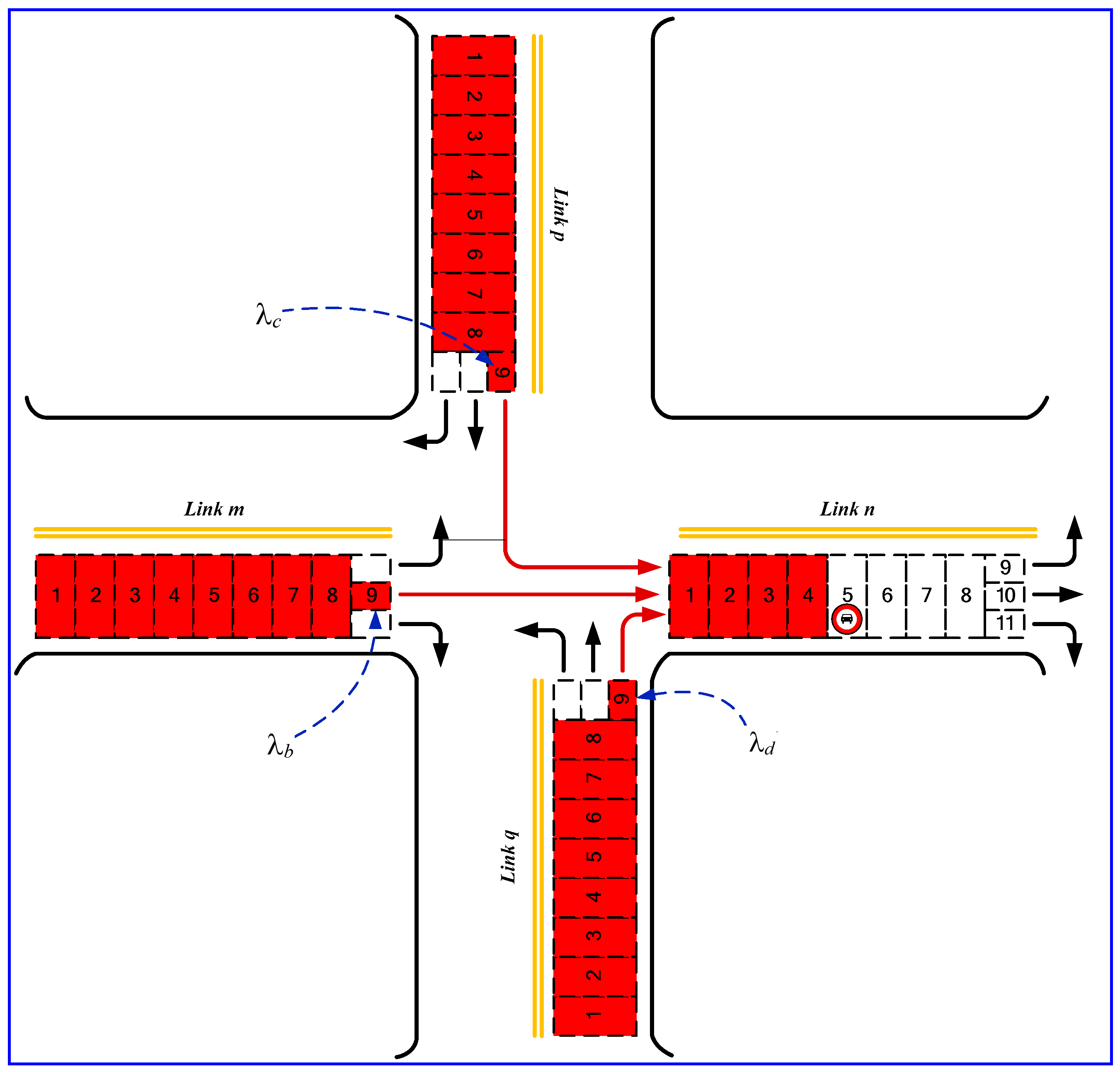
To better explain the challenges associated with the traditional CTM method, we will first outline the reasons why calibration is necessary. Using Figure 2 as an example, we illustrate the need for calibration. Suppose a traffic road (link n) is blocked due to an accident occurring in the fifth cell of link n. We then calculate the number of jammed cells with parameters φ_ac = 0.2, φ_ab = 0.5, and φ_ad = 0.3. Based on these calculations, we generate a jam propagation diagram, as shown in Figure 2, which visually captures the process of congestion growth. The results reveal that once link n becomes congested, the congestion spreads to other links m, p, and q, leading to a network-wide traffic jam. However, in real-world traffic scenarios, congestion in a left-turn or right-turn lane should not necessarily result in the complete blockage of an entire road segment. This discrepancy indicates that the results obtained from the traditional CTM method do not accurately reflect actual road traffic conditions. To address this limitation, we propose a new vehicle allocation rule that improves upon the shortcomings of the traditional CTM method.

It is obvious that the actual road traffic need not cause congestion of the entire road because of the congestion of the left/right turning lane. Hence, we believe that the results calculated based on the traditional CTM method do not match actual road traffic conditions. Therefore, we propose a new vehicle allocation rule to address the lacunae of the traditional CTM method.

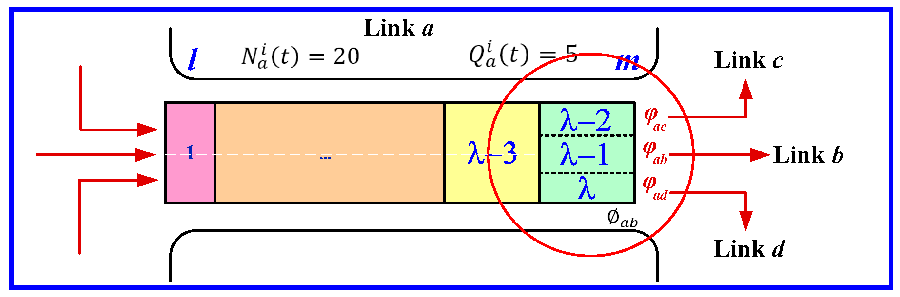
3.2. Downstream Queue Area of the Calibrated CTM Method

Considering the limitations of traditional CTMs, we modify the three sub-cells λ_b, λ_c, and λ_d into independent cells λ − 2, λ − 1, and λ, respectively. Figure 3 illustrates the modified downstream queues of link a. Moreover, the maximum number of vehicles that can occupy cell i of link a is specified as ${ N}_a^i\left(t\right)=20, where i\in \{1,2,\dots ,\mathrm{\lambda }\}$.

However, we notice that the upstream cell has two lanes, whereas the downstream cell has three lanes, but the capacity of the lanes to accommodate vehicles remains unchanged. The definition of the traditional CTM method does not appear to consider the number of different lanes. Therefore, we try to modify ${\mathrm{N}}_{\mathrm{a}}^{\mathrm{i}}\left(t\right)=20, \mathrm{i}\in \{1,2,\dots ,\mathrm{\lambda }\}$ into ${\mathrm{N}}_{\mathrm{a}}^{\mathrm{i}}\left(t\right)=20, \mathrm{i}\in \left\{1,2,\dots ,\mathrm{\lambda }-3\right\}$ and ${\mathrm{N}}_{\mathrm{a}}^{\mathrm{i}}\left(t\right)=10, \mathrm{i}\in \{\mathrm{\lambda }-2,\mathrm{\lambda }-1,\mathrm{\lambda }\}$.

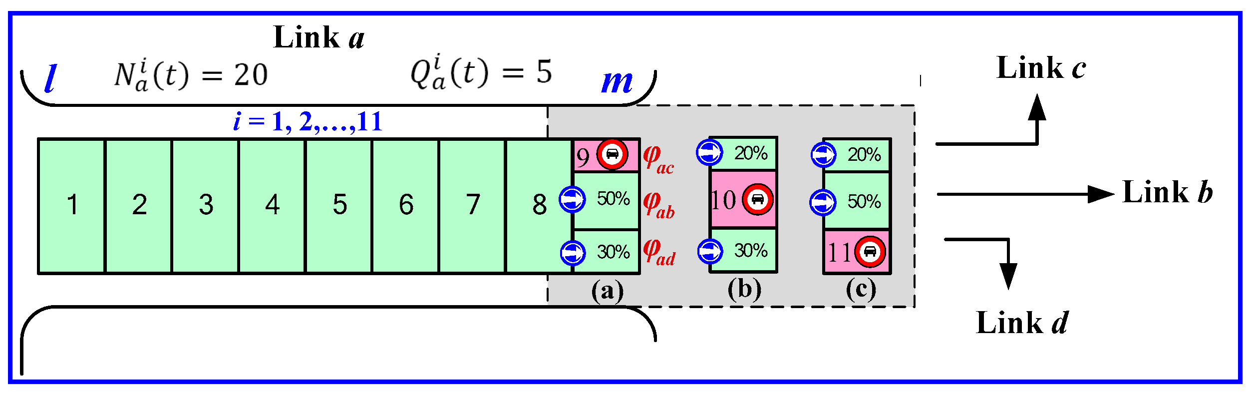
Three cases of jammed cells are discussed below. Specifically, with λ = 11, we assign λ − 2, λ − 1, and λ to the left-turn lane, straight lane, and right-turn lane, respectively.

• Case I: Left-Turn Lane Jammed

Figure 4a shows that once downstream cell 9 is jammed, we stop upstream cell 8 from allocating vehicles to enter downstream cell 9. Based on the proportion of vehicles turning left, turning right, and going straight, we allow 50% of the upstream vehicles to be allocated to the downstream straight lane and 30% to the right-turn lane. Note that this allocation rule is different from the strategy used in the traditional CTM method.

• Case II: Straight Lane Jammed

Figure 4b shows that once downstream cell 10 is jammed, we stop upstream cell 8 from allocating vehicles to enter downstream cell 10. Then, we allow 20% of the upstream vehicles to be allocated to downstream cell 9 (i.e., the left-turn lane) and 30% to downstream cell 11 (i.e., the right-turn lane).

• Case III: Right-Turn Lane Jammed

Figure 4c shows that once downstream cell 11 is jammed, we stop upstream cell 8 from allocating vehicles to enter downstream cell 11. Then, we allow 50% of the upstream vehicles to be allocated to the downstream straight lane (i.e., cell 10) and 20% to the left-turn lane (i.e., cell 9).

Based on the traditional CTM method, if congestion occurs in any of the three lanes (i.e., left-turn, right-turn, or straight lane) when vehicles are moving forward downstream, the method restricts the upstream vehicles from entering downstream cell 9. This highlights an important relationship between the upstream and downstream cells. When vehicles move from the upstream cell (λ − 3) to the downstream cells (λ − 2, λ − 1, or λ), two key factors must be considered: the vehicle density in each downstream cell and the number of vehicles in the upstream cell. To better reflect real-world road conditions, we appropriately calibrate the parameter φ_ax. Figure 2 illustrates how congestion in any downstream lane can lead to congestion in the entire upstream lane. However, unlike the traditional CTM method, our improved approach allows vehicles to move into uncongested lanes. Even if two of the three lanes are jammed, vehicles can still enter the remaining open lane. Notably, the traditional CTM method would restrict movement into any downstream lane, even if it remains uncongested.

To illustrate how our new CTM method operates, we designed a pseudocode to explain the updated vehicle allocation rules, as shown in Algorithm 2. This pseudocode shows that if the capacity of any downstream cell is not full, i.e., $n_a^{\mathrm{\lambda }}, \mathrm{\lambda }$ ∈ {9, 10, 11}, then the upstream cell (cell 8) will allocate vehicles accordingly. Notably, this new CTM method differs significantly from the traditional approach. For convenience, we use the notation φ_{λ∈{9, 10, 11}} to replace φ_ac, φ_ab, and φ_ad. Here, Nφ_λ represents the maximum number of vehicles that can be contained in cell λ at a given time interval.

Algorithm 2. A new vehicle allocation rule of the CTM

# Input vehicles to downstream cells def distribute_vehicles(n_a, N_φ):        # Check if any downstream cell (λ ∈ {9, 10, 11}) is not full        if n_a[9] ! = N_φ[9] or n_a[10] ! = N_φ[10] or n_a[11] ! = N_φ[11]:          return φ_9 + φ_10 +φ_11 # Distribute vehicles        # Check conditions for each cell step by step        if n_a[9] == N_φ[9]:          if n_a[10] == N_φ[10]:            if n_a[11] == N_φ[11]:              return φ_9 + φ_10 + φ_11            else:              return φ_9 + φ_10 + φ_11          else:            if n_a[11] == N_φ[11]:              return φ_9 + φ_10 + φ_11            else:              return φi_9 +φ_10 + φ_11        else:          if n_a[10] == N_φ[10]:            if n_a[11] == N_φ[11]:              return φ_9 + φ_10 + φ_11            else:              return φ_9 + φ_10 + φ_11          else:            if n_a[11] == N_φ[11]:              return φ_9 + φ_10 + φ_11            else:              return φ_9 + φ_10 + φ_11

For example, if N = 10 and φ₉ = 0.2, φ₁₀ = 0.5, and φ₁₁ = 0.3, then we can determine the following:

If $n_a^9<$ N × φ₉, $n_a^{10}<$ N × φ₁₀, and $n_a^{11}<$N × φ₁₁, then $y_a^9, y_a^{10}$, and $y_a^{11}$ will be nonzero. This means that the upstream cell can allocate vehicles to all three downstream cells.

If $n_a^9=$ N × φ₉, $n_a^{10}<$ N × φ₁₀, and $n_a^{11}<$ N × φ₁₁, then $y_a^9=0 while y_a^{10}\ne 0$ and $y_a^{11}\ne 0$. This indicates that the upstream cell will allocate vehicles only to cells 10 and 11.

If all downstream cells are at full capacity, i.e., $n_a^{\mathrm{\lambda }}, \mathrm{\lambda }$ ∈ {9, 10, 11}, then the upstream cell will stop allocating vehicles. Furthermore, if N × φ₉ = 2, the upstream cell will stop allocating vehicles to cell 9, meaning that the left-turn lane has reached its maximum capacity of two vehicles and is now congested. Conversely, if N × φ₉ < 2, the upstream cell can still allocate vehicles to cell 9, indicating that the left-turn lane is not yet fully congested. In this case, vehicles from upstream cell 8 can still enter the left-turn lane.

4. Simulation of Traffic Jam Propagation and Dispersion

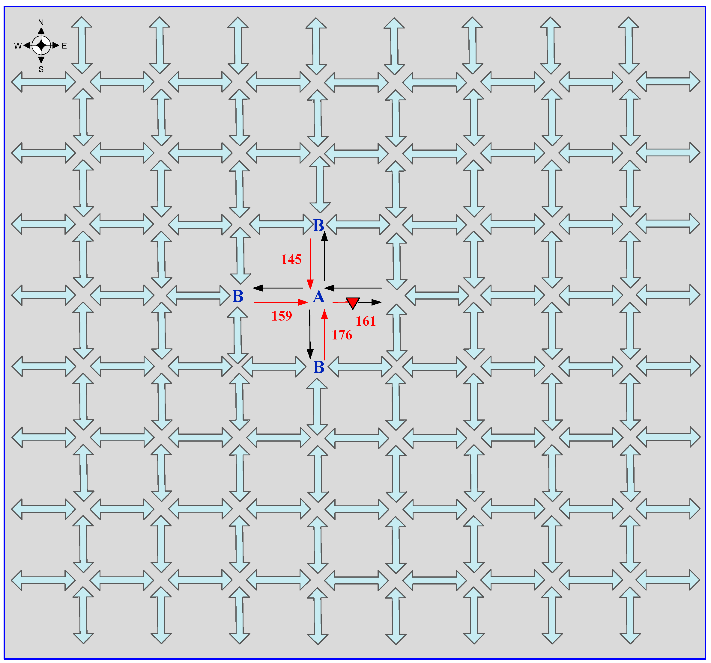
Based on the definition provided above, we developed a time-step-based traffic simulation environment using MATLAB to model traffic jam propagation and dispersion. This simulation is built on the CTM, allowing for a detailed representation of realistic traffic dynamics. In Figure 5, we illustrate a two-way 8 × 8 grid traffic network to demonstrate how traffic congestion spreads after an accident. In this 8 × 8 grid network model, each pair of adjacent vertices (intersections) is connected by two unidirectional links (one for each direction of traffic flow). This bidirectional design ensures a realistic representation of urban grid networks, where vehicles move independently in opposing directions.

In this network, all boundary nodes are considered start and end points. The inverted triangle in Figure 5 marks the location of an accident on link 161. The network is made up of 288 links, each divided into 11 cells. For a more detailed analysis of traffic behavior, each link is also split into two zones: (1) an upstream zone containing eight cells and (2) a downstream zone containing three cells. This structured approach allows for a more precise simulation of congestion dynamics and how traffic conditions evolve over time.

For simplicity, the extended CTM parameters are set as in [14,27]:

Time interval: 5 s.

Jam density: 133 vehicles/km (7.5 m/vehicle).

Free-flow speed: 54 km/h (15 m/s).

Backward shock-wave speed: 21.6 km/h (6 m/s).

Number of lanes: two.

Flow capacity: 1800 vehicles/h/lane.

Cell length: 75 m, holding capacity: 20 vehicles.

Number of cells per link: nine (link length: 675 m).

A cell is considered jammed as follows:

The density in the upstream ‘reservoir’ > 0.9 N.

The density in any downstream direction > 0.9 k_j.

We assume that the initial state of the 8 × 8 grid road network is empty. For the purpose of comparison, the analysis period is set to 4000 time intervals, with an accident occurring in the central zone of the network, specifically at the fifth cell of link 161. A cell is considered jammed if its density exceeds 0.9 N [14]. To assess the effectiveness of different strategies, we use two traffic flow conditions, i.e., t_d = 0.75 and t_d = 0.8, where t_d represents the number of vehicles per time interval. For example, t_d = 0.75 indicates that three vehicles enter each entrance every 20 s.

Recently, Qi et al. [10] introduced a two-level strategy, known as the Q-strategy, to prevent urban traffic congestion caused by accidents. This strategy assumes that when a ban signal is shown for a particular direction, d_A% of the vehicles will reroute and d_B% will reroute when a warning signal is displayed. The ban signal serves as the first level, stopping traffic from heading toward an accident, while the warning signal acts as the second level, advising drivers against taking that route. To enhance accident-based congestion prevention, we present an innovative three-level control strategy, the H-strategy, which employs ban and warning signals at adjacent intersections to redirect traffic away from the accident area. For consistency, in our simulation, we use the parameter values provided by Qi et al. [10]. While their approach applies a ban signal at intersection A and a warning signal at intersection B, our method enforces ban signals at intersection A to halt accident-bound traffic and extends warning signals to adjacent intersections B and C, advising drivers to avoid the affected direction. In this study, we use d_A, d_B, and d_C to denote the percentage of vehicles rerouting at intersections A, B, and C, respectively. We present two examples to illustrate the behavior of the traditional and calibrated CTM methods under different conditions.

• Example 1 [34]:

This example illustrates the differences between traditional vehicle allocation rules 6 and our new allocation rules 6. We analyze traffic jam formation and dispersion using three strategies, i.e., no strategy, Q-strategy, and H-strategy, under both the traditional and calibrated CTM methods. In this case, an accident occurs between the 301st and 1500th time intervals. Here, d_A = 1.0 with d_B = 0.6 and d_C = 0.8 are for the Q-strategy, and d_A = 1 and d_B = d_C = 0.8 are for the H-strategy. 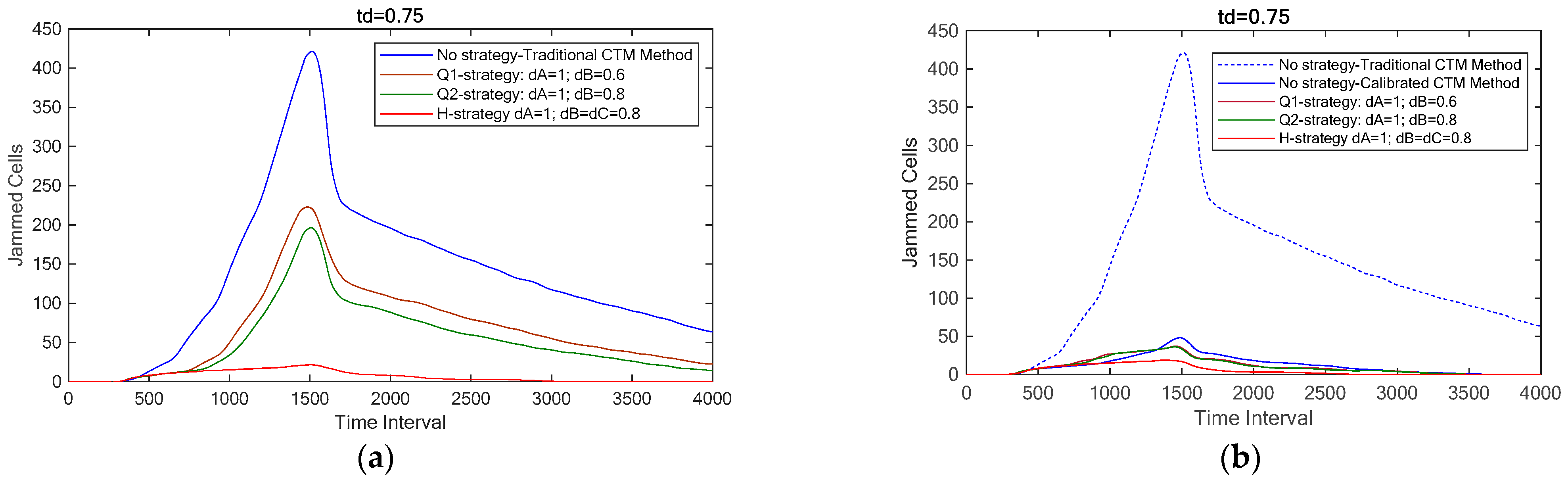Figure 6a shows traffic jam propagation and dispersion using the traditional CTM method with t_d = 0.75, based on parameters from Luo et al. [17]. For comparison, Figure 6b presents the simulation results for both the traditional and calibrated CTM methods, also with t_d = 0.75.

A key observation is the significant difference between the blue dashed and solid lines. The dashed line shows that the traffic jam starts at the 343rd time interval and peaks at 421 jammed cells by the 1513th interval. In contrast, the solid line shows a jam initiation at the same time but with a peak of only 48 jammed cells at the 1486th interval.

For the Q1-strategy, Q2-strategy, and H-strategy, traffic jams start at the 341st, 338th, and 337th time intervals, respectively, with peak jammed cells of 37 (1460th interval), 36 (1453rd interval), and 19 (1386th interval). The results indicate that the H-strategy (d_A = 1 and d_B = d_C = 0.8) outperforms the other two Q-strategy conditions (d_A = 1.0 with d_B = 0.6; 0.8). Overall, any controlled strategy significantly reduces the congestion duration compared to having no strategy. Additionally,

Table 2. Number of jammed cells and their corresponding time interval details for example 1.

Time interval	500	1500	2500	3500	500	1500	2500	3500
Strategy	Traditional CTM (td = 0.75)				Calibrated CTM (td = 0.75)
No strategy N = 20	13	421	155	90	8	48	11	1
Q1: dA = 1; dB = 0.6	7	222	79	37	7	35	8	0
Q2: dA = 1; dB = 0.8	8	196	59	26	8	33	6	0
H-strategy dA = 1; dB = dC = 0.8	8	21	2	0	8	17	1	0

confirms that the H-strategy is more effective than both the Q1- and Q2-strategies.

• Example 2:

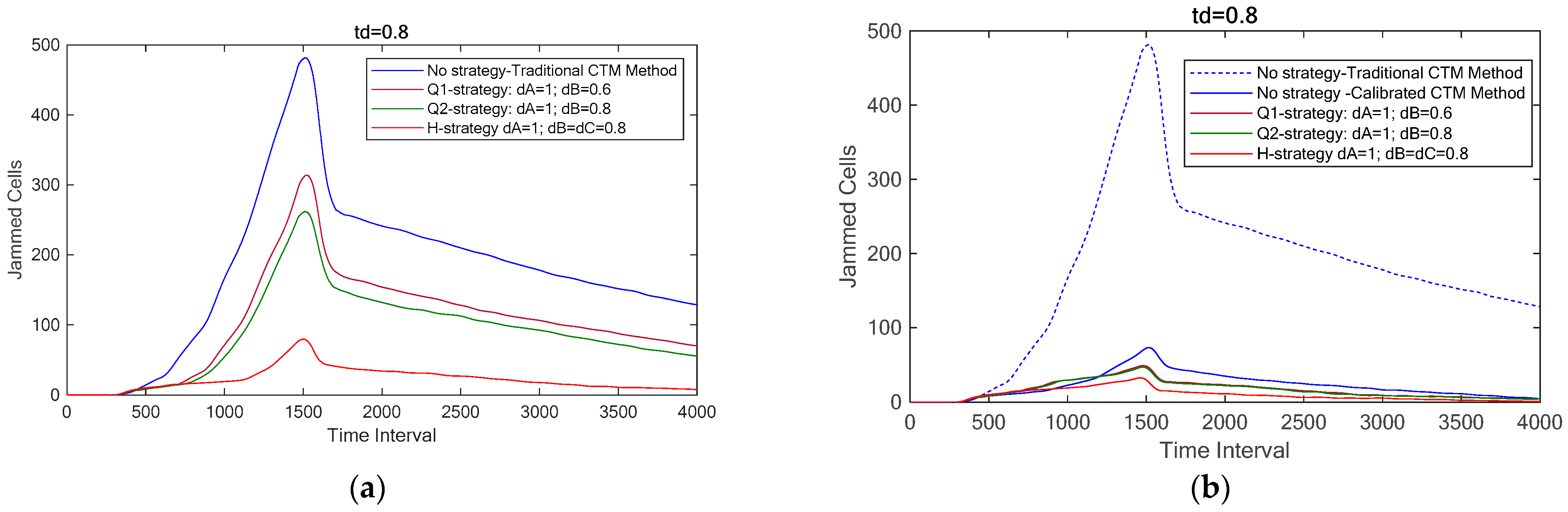
The two vehicle allocation rules, along with t_d = 0.8, are simulated to analyze traffic jam formation and dispersion under identical accident conditions. Figure 7a presents four simulation results, where the traffic jam starts at the 339th time interval with no strategy and peaks at 481 jammed cells by the 1515th interval. Notably, it takes over 4000 time intervals for dispersion. Similarly, both CTM methods with t_d = 0.8 are simulated together, with the results shown in Figure 7b.

The blue dashed line in Figure 7b shows that the traffic jam starts at the 339th interval and peaks at 481 jammed cells at the 1515th interval. In contrast, the blue solid line indicates a later onset at the 342nd interval, with a significantly lower peak of 73 jammed cells at the 1516th interval. For the Q1-strategy, Q2-strategy, and H-strategy, traffic jams begin at the 338th, 333rd, and 332nd intervals, respectively, with peak jammed cells of 49 (1479th interval), 47 (1476th interval), and 33 (1461st interval). The results confirm that the H-strategy outperforms the Q1- and Q2-strategies in traffic jam dispersion. Overall, any controlled strategy significantly reduces the congestion duration compared to having no strategy. Additionally,

Table 3. Number of jammed cells and their corresponding time interval details for example 2.

Time interval	500	1500	2500	3500	500	1500	2500	3500
Strategy	Traditional CTM (td = 0.8)				Calibrated CTM (td = 8)
No strategy N = 20	14	480	210	152	8	73	25	11
Q1: dA = 1; dB = 0.6	8	310	128	88	8	48	15	7
Q2: dA = 1; dB = 0.8	9	261	113	72	9	46	14	6
H-strategy dA = 1; dB = dC = 0.8	10	80	27	11	10	30	6	2

indicates that the H-strategy consistently delivers the best performance, regardless of whether t_d = 0.75 or t_d = 0.8.

5. Conclusions

This study highlights that traffic incidents are a major cause of congestion and examines the limitations of the Cell Transmission Model (CTM) in accurately simulating traffic jams. While the CTM is widely used, it exhibits two key inaccuracies, emphasizing the need for proper calibration and validation. To address this, we embedded a calibrated CTM into a MATLAB-based simulation of an 8 × 8 grid traffic network to analyze accident-induced congestion. Only cell 9 was divided into three smaller cells to represent different movement directions (left-turn, go-straight, and right-turn), ensuring a more accurate depiction of traffic flow. This refinement maintains the standard nine-cell structure elsewhere, balancing computational efficiency with improved intersection modeling. Through two case studies, we compared the traditional and calibrated CTM methods under different traffic conditions. The results revealed that the traditional CTM method often underestimates or overestimates congestion spread and dissipation, leading to unrealistic traffic flow predictions. In contrast, the calibrated CTM method provided more precise estimations, better capturing the dynamic nature of traffic jams. Specifically, the calibrated CTM showed a more accurate representation of queue formation, shockwave propagation, and clearance time, resulting in improved decision-making for traffic control strategies.

Here, we explicitly highlight the originality and significance of our research by emphasizing the following key contributions: (1) Introducing a novel refinement to the traditional CTM by dividing only cell 9 into three smaller cells to accurately capture different movement directions, enhancing intersection modeling without increasing overall computational complexity. (2) Identifying critical inaccuracies in the conventional CTM when modeling accident-induced congestion, addressing limitations in congestion propagation and dissipation. (3) Proposing a calibrated CTM framework that significantly improves the representation of congestion dynamics, offering a more realistic depiction of traffic flow disruptions. (4) Demonstrating the effectiveness of the novel H-strategy, which outperforms the existing control methods in mitigating congestion and improving network performance.

Our future research directions include the following:

Scalability to complex networks: Extending the calibrated CTM framework to three-way or four-way grid networks and non-uniform urban layouts, incorporating dynamic lane configurations.

Resilience to extreme disruptions: Integrating real-time adaptive mechanisms to address unexpected events (e.g., earthquakes, accidents) and evaluating the H-strategy’s performance under stochastic demand fluctuations.

Human behavior integration: Enhancing the model to account for heterogeneous driver decisions (e.g., route diversion, compliance variability) using agent-based modeling or empirical trajectory data.

Emerging technologies: Exploring synergies between the calibrated CTM and connected/autonomous vehicle (CAV) systems to optimize traffic control strategies in mixed traffic environments. These advancements will further bridge the gap between theoretical models and practical traffic management applications, enabling cities to adopt proactive, data-driven strategies for congestion mitigation.