Improving Vertebral Fracture Detection in C-Spine CT Images Using Bayesian Probability-Based Ensemble Learning

Abstract

Vertebral fracture (VF) may induce spinal cord injury that can lead to serious consequences which eventually may paralyze the entire or some parts of the body depending on the location and severity of the injury. Diagnosis of VFs is crucial at the initial stage, which may be challenging because of the subtle features, noise, and homogeneity present in the computed tomography (CT) images. In this study, Wide ResNet-40, DenseNet-121, and EfficientNet-B7 are chosen, fine-tuned, and used as base models, and a Bayesian-based probabilistic ensemble learning method is proposed for fracture detection in cervical spine CT images. The proposed method considers the prediction’s uncertainty of the base models and combines the predictions obtained from them, to improve the overall performance significantly. This method assigns weights to the base learners, based on their performance and confidence about the prediction. To increase the robustness of the proposed model, custom data augmentation techniques are performed in the preprocessing step. This work utilizes 15,123 CT images from the RSNA-2022 C-spine fracture detection challenge and demonstrates superior performance compared to the individual base learners, and the other existing conventional ensemble methods. The proposed model also outperforms the best state-of-the-art (SOTA) model by 1.62%, 0.51%, and 1.29% in terms of accuracy, specificity, and sensitivity, respectively; furthermore, the AUC score of the best SOTA model is lagging by 5%. The overall accuracy, specificity, sensitivity, and F1-score of the proposed model are 94.62%, 93.51%, 95.29%, and 93.16%, respectively.

1. Introduction

The spine consists of a stack of several bones of different shapes known as vertebrae. The uppermost seven vertebrae, ranging from C1 to C7 of the spine are called the cervical spine (C-spine). The vertebrae protect the spinal cord from injury and also support the stability of the entire body [1]. Any serious vertebral injury might lead to spinal cord injury (SCI), and that might have severe consequences [2].

A recent study reported that, out of the total SCI diagnosed each year, 55% belonged to C-spine injury (CSI) [3]. Any vertebral injury may lead to life-threatening conditions due to dysfunction of the nervous system [4]. The cause of vertebral fracture (VF) may be traumatic or non-traumatic. The major traumatic causes include vehicular accidents, falls, gunshot injuries, herniated discs, heavy lifting, and sudden movements that strain the back whereas, the non-traumatic causes are osteoporosis, vascular events, and degenerative disc disease [5].

The initial diagnosis of VF is primarily conducted using a CT scan, and a well-trained radiologist is required to distinguish between a fracture image and a non-fracture image. However, it often creates challenges to the radiologist due to the low spatial resolution of CT images which is the consequence of low radiation dose during the image acquisition. Recent advancements in computing power have enabled the development of software-based methods for iterative image reconstruction in CT, enabling simultaneous reduction of noise and improvement of overall image quality. Additional details on iterative methods are found in [6,7,8,9].

The incidence of spinal trauma and subsequent VFs is steadily increasing day by day [10]. Fast diagnosis of VF can significantly accelerate treatment planning and save millions of lives [11]. The manual diagnosis of CSI, particularly the subtle fractures, can be challenging and time-consuming due to the noise, homogeneity between fracture and non-fracture regions, and low-level features in CT images. Small fractures are not immediately apparent on initial examination; however, they still can cause significant pain and may lead to other complications if not treated in a timely way.

Artificial intelligence (AI) has significantly contributed in medical imaging, supporting various applications like lesion detection, disease classification, quantification, and segmentation [12]. Some previous work on the application of AI in spine injury and recent advancements of deep learning in this area are discussed below.

In a study by Shaolong et al. [13], CSI was detected using Faster-RCNN, where VGG-16 and ResNet-50 were used for feature extraction, achieving 72.3% and 88.6% mean average precision (mAP), respectively. However, the study was conducted on a dataset obtained from a single modality in a hospital, which hindered the generalizability of the model.

In another study, C-spine fractures were detected using a convolutional neural network (CNN) developed by Aidoc. However, the model failed to detect acute fracture-dislocation, and any injuries in the lower C-spine [14].

In another work [15], vertebral compression fracture (VCF) was detected using mask R-CNN in which ResNet-101 was utilized for feature extraction, followed by a region proposal network to capture the affected area. The accuracy of their model was merely 80.4%.

In [16], an ensemble learning approach, majority voting, was utilized to detect the VCF in the thoracic spine. However manual annotation was performed for all the images, which was time-consuming, and an accuracy of 86.67% was achieved.

In a study conducted by Xu et al. [17], an AI-based VCFs detection model was developed using X-ray images. The basic and shallow ResNet-18 was used as a base model which managed to achieve a low accuracy of 82.9%.

A deep CNN was developed for VF detection using plain abdominal radiographs, achieving accuracy, specificity, sensitivity, and AUC of 73.59%, 73.02%, 73.81%, and 72%, respectively. While it demonstrated fair performance, it was solely trained on plain radiographs [18]. In [19], Chen et al. proposed a method for VCF detection and obtained 74% accuracy, 68% specificity, and 80% sensitivity with an AUC of 89%. Despite moderate performance, both models lack robustness and generalization, as they worked on a small dataset obtained from a single modality.

In another study [20], a model was proposed to detect osteoporotic VF and utilized the fusion of three CNNs, achieving accuracy, specificity, sensitivity, and AUC of 89%, 92%, 83%, and 87.6%, respectively. However, the model was trained on only the bone part of the vertebral images, obtained using the YOLOv5 object detection model, indicating that it will not be useful for real-time applications as clinical images contain bone structure, soft tissue, and other background parts. Furthermore, their ensemble approach was not made explicit, so systematically combining predictions from CNNs may be more useful in improving the result.

A CNN-based model for VF detection using CT images was developed by Nicolaes et al. [21], achieving 93% accuracy, 93% specificity, 94% sensitivity, and an AUC of 94%. While the model shows promising results, the study was conducted on a small dataset, which may restrict the generalizability.

A generative adversarial network (GAN)-assisted CNN was developed to detect VF, which improved classification accuracy from 73% to 89% and achieved an F1-score of 90%. However, more synthetic images might distort the model’s learning capabilities, and make it less reliable for real-world application. Handling the uncertainties about the model’s prediction would be beneficial in this case [22].

Guenoun et al. [23] proposed a method for VCF detection using CT scans and achieved 92% accuracy, 91.7% specificity, and 92.3% sensitivity. While it has impressive performance, the model focuses primarily on patients above 50 years who have undergone chest-abdominal-pelvis CT scans obtained from a single modality from a hospital, which suggests the model might not be robust.

Although AI has made significant contributions in various areas pertinent to the medical field, its use, specifically, in detecting C-spine vertebral fractures, is in the nascent stage. AI-assisted methods could be useful in the early detection of vertebral injuries for effective treatment and management in such cases. A recent survey found that a few studies had been undertaken on AI-assisted vertebral fracture detection by 2022 [24]. The present study aims to design and evaluate an AI-based model to detect fractures in C-spine vertebrae using CT images. The major contributions of this work are summarized as follows:

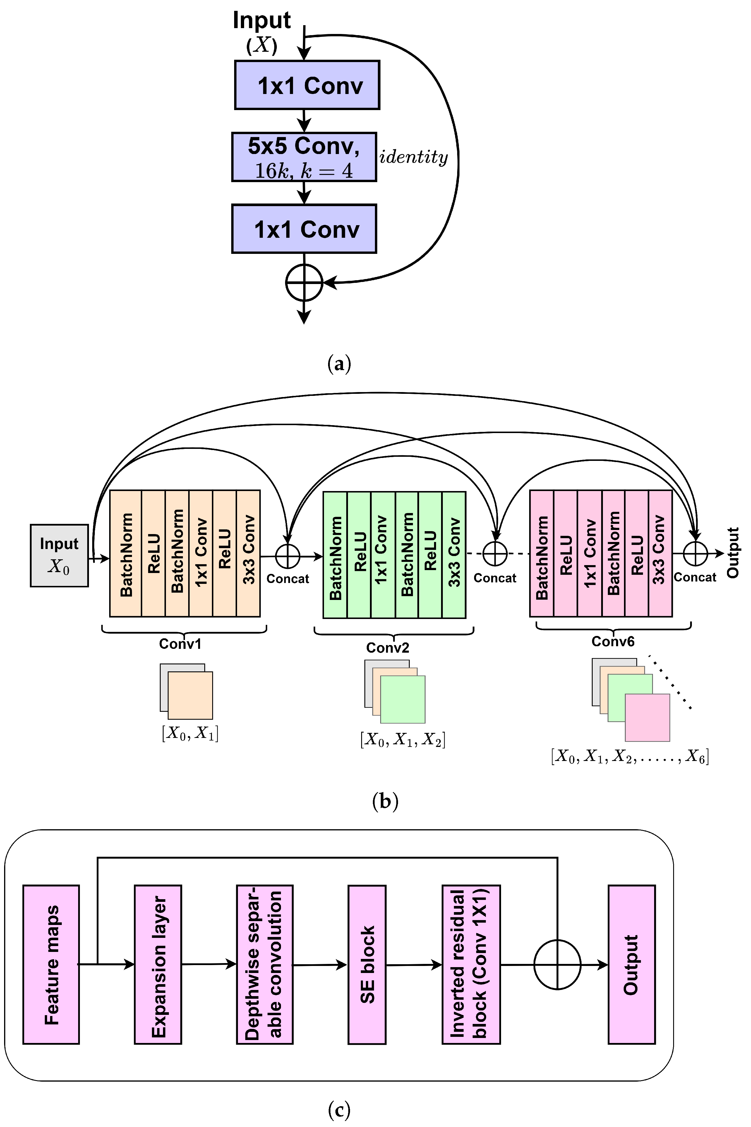
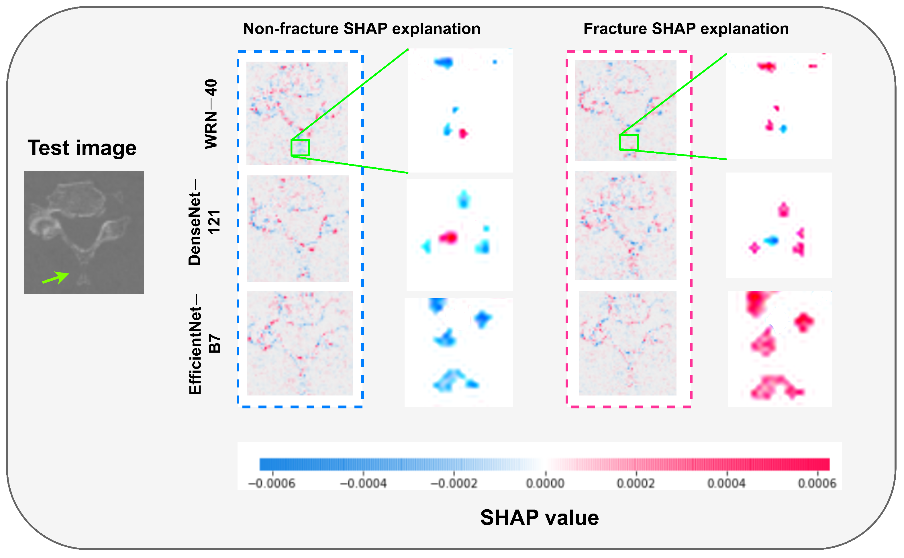
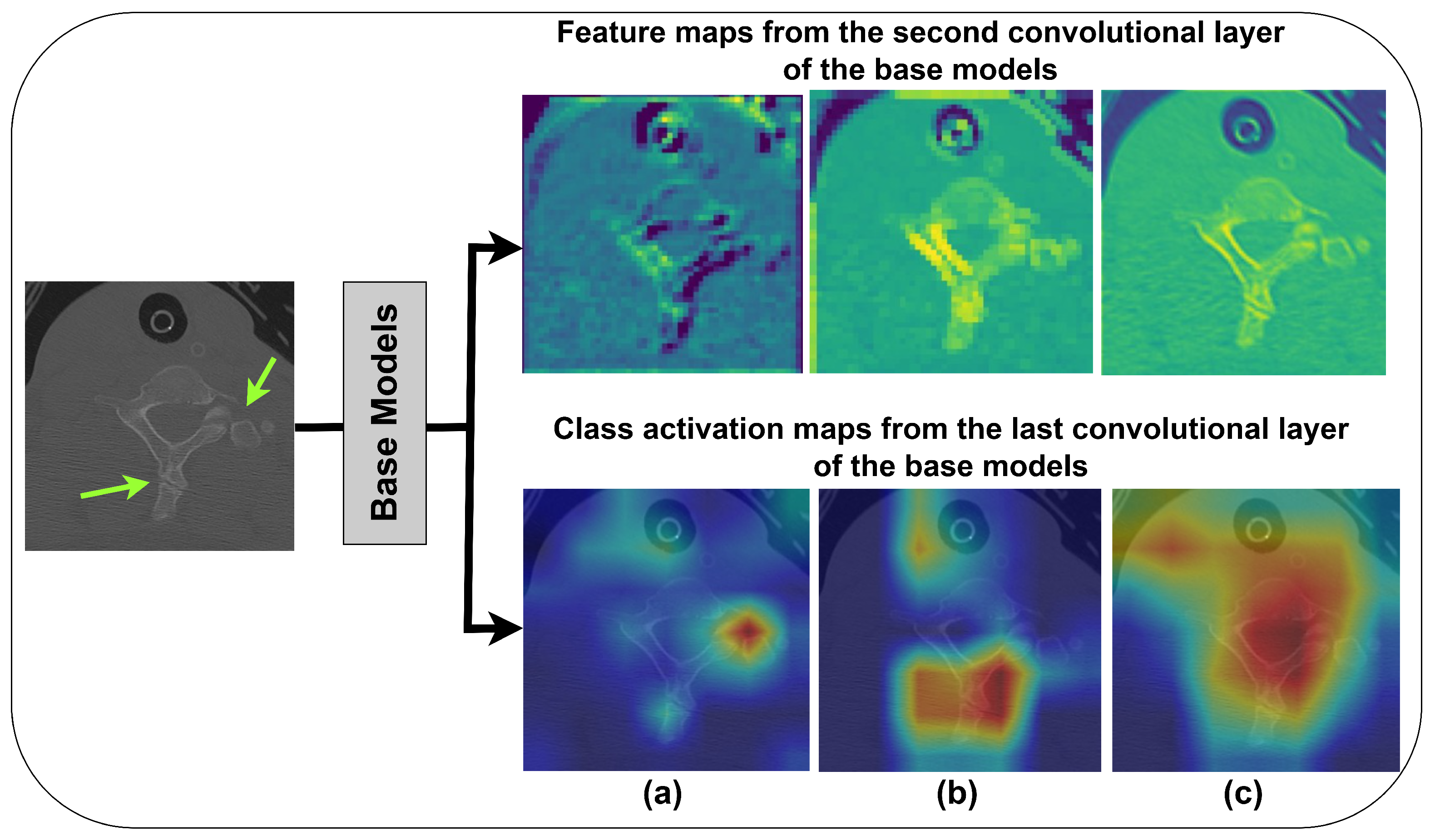
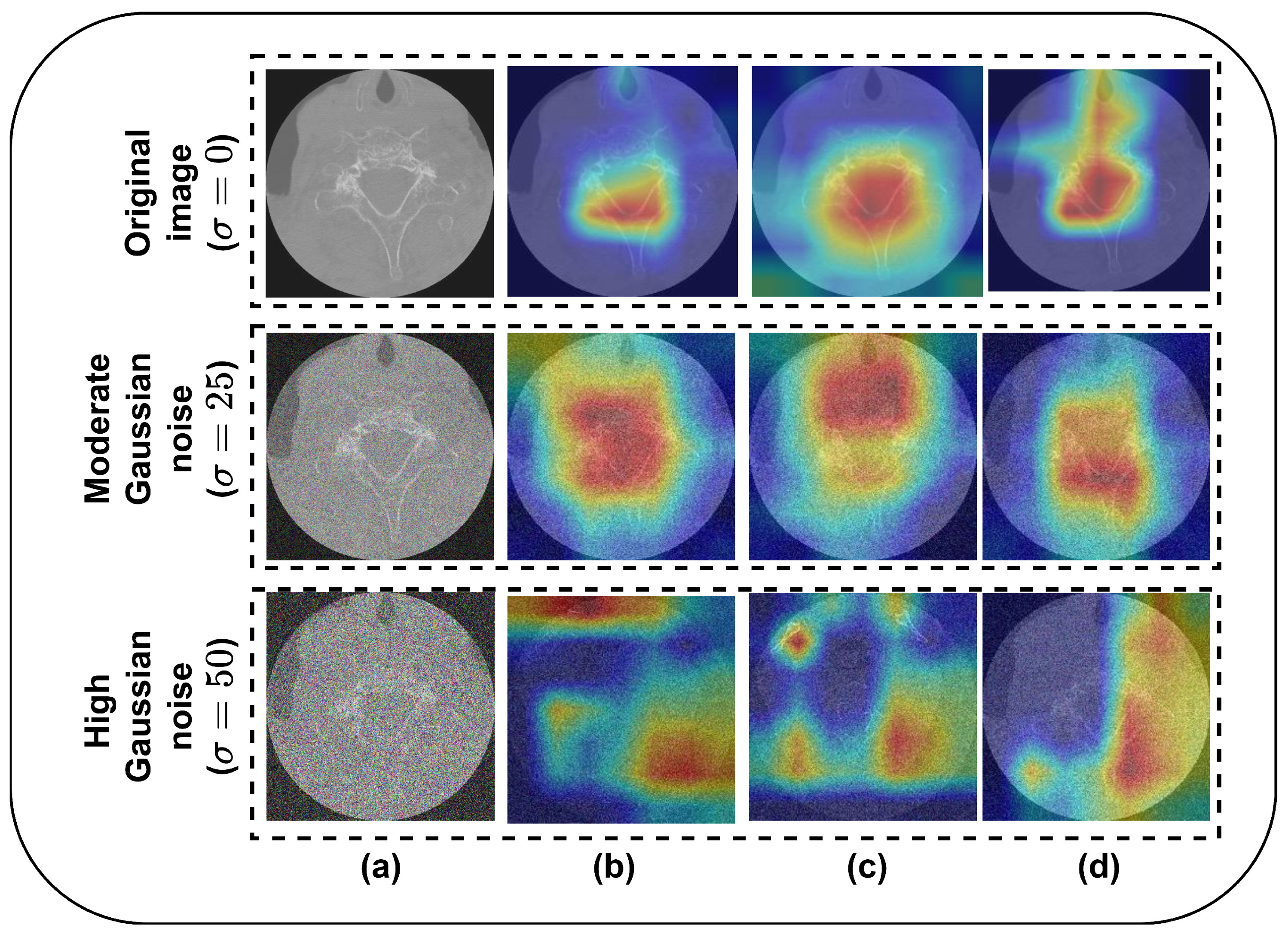
• Training and fine-tuning of three CNNs with 5-fold cross-validation (CV) for VF detection using C-spine CT images and employing them as base learners. Additionally, a base model interpretability analysis is conducted using SHapley Additive exPlanations and the Grad-CAM method.
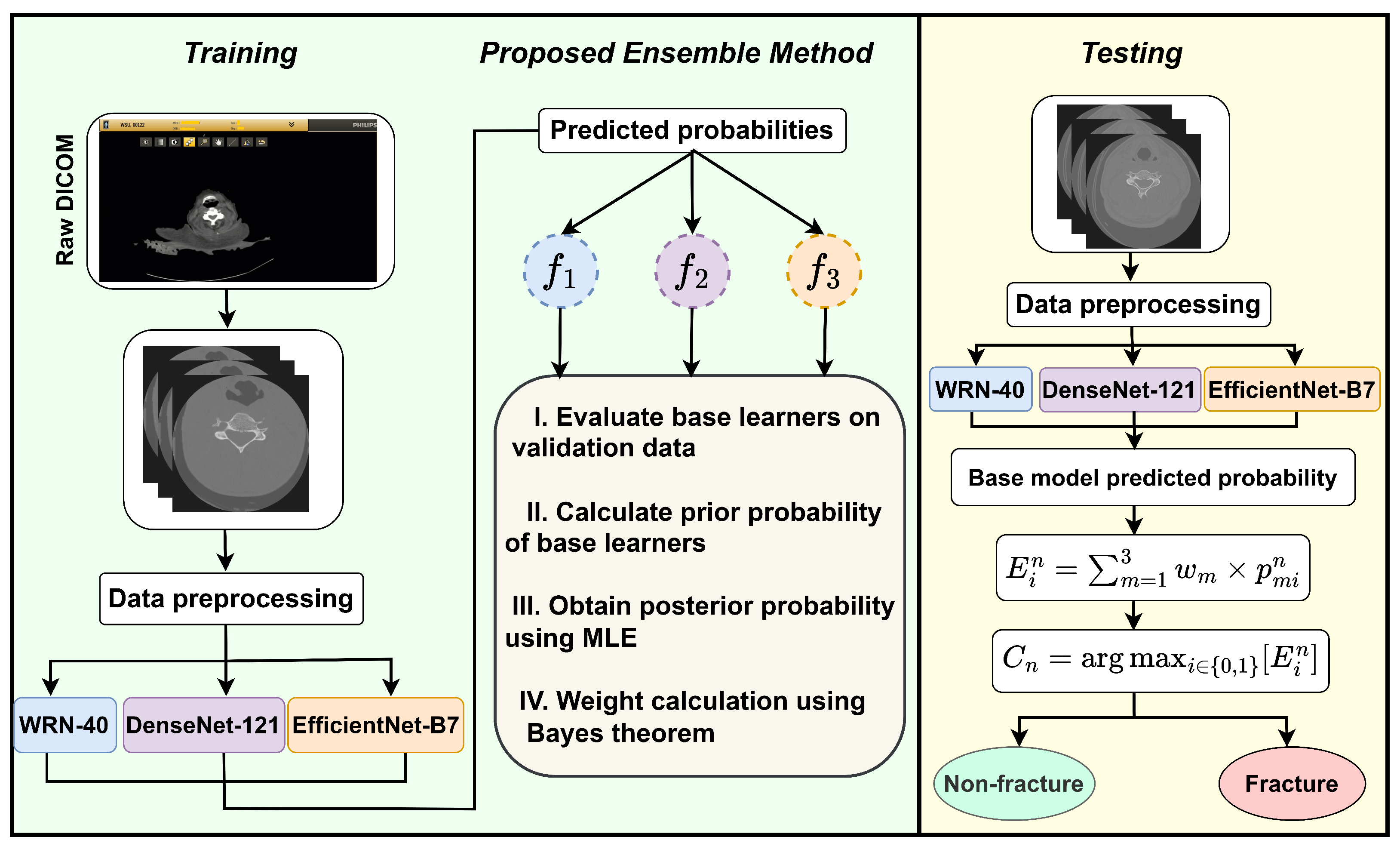
• To improve the classification performance, a novel ensemble learning approach based on Bayesian probability is proposed.
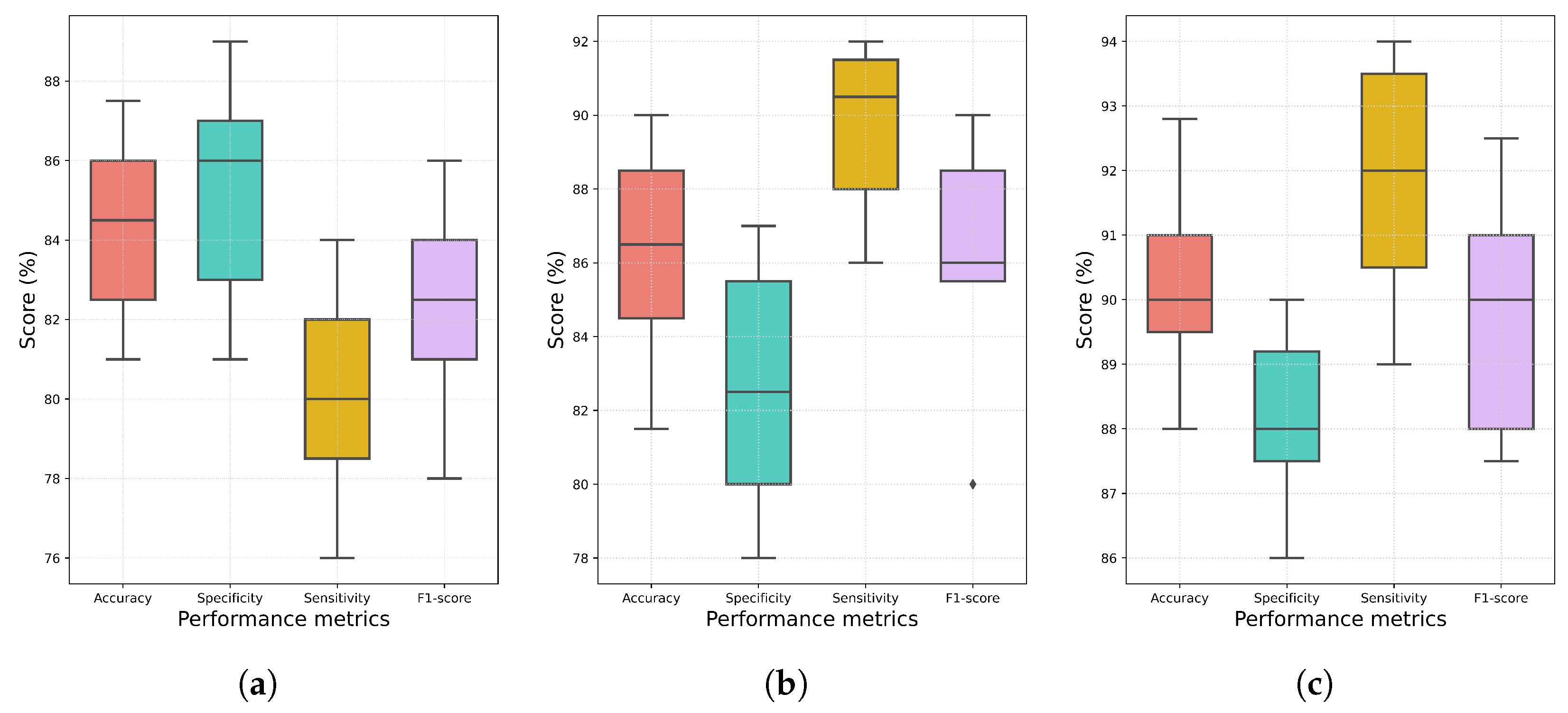
• To validate the potential of the proposed framework, conventional ensemble learning methods are implemented on our dataset, and then their performance is analyzed and compared with the proposed model in terms of accuracy, specificity, sensitivity, and the F1-score.

The rest of the paper is structured as follows: The data preprocessing, base model training with hyperparameter optimization, and proposed methodology are explained in Section 2. The comparative analysis of results of the proposed model with base models and other traditional ensemble learning methods is reported in Section 3. The conclusions, limitations, and future scope of this study are discussed in Section 4.

2. Materials and Methods

This section focuses on data preprocessing, data augmentation, base model training, and their hyperparameter optimization. The proposed methodology is also discussed in this section.

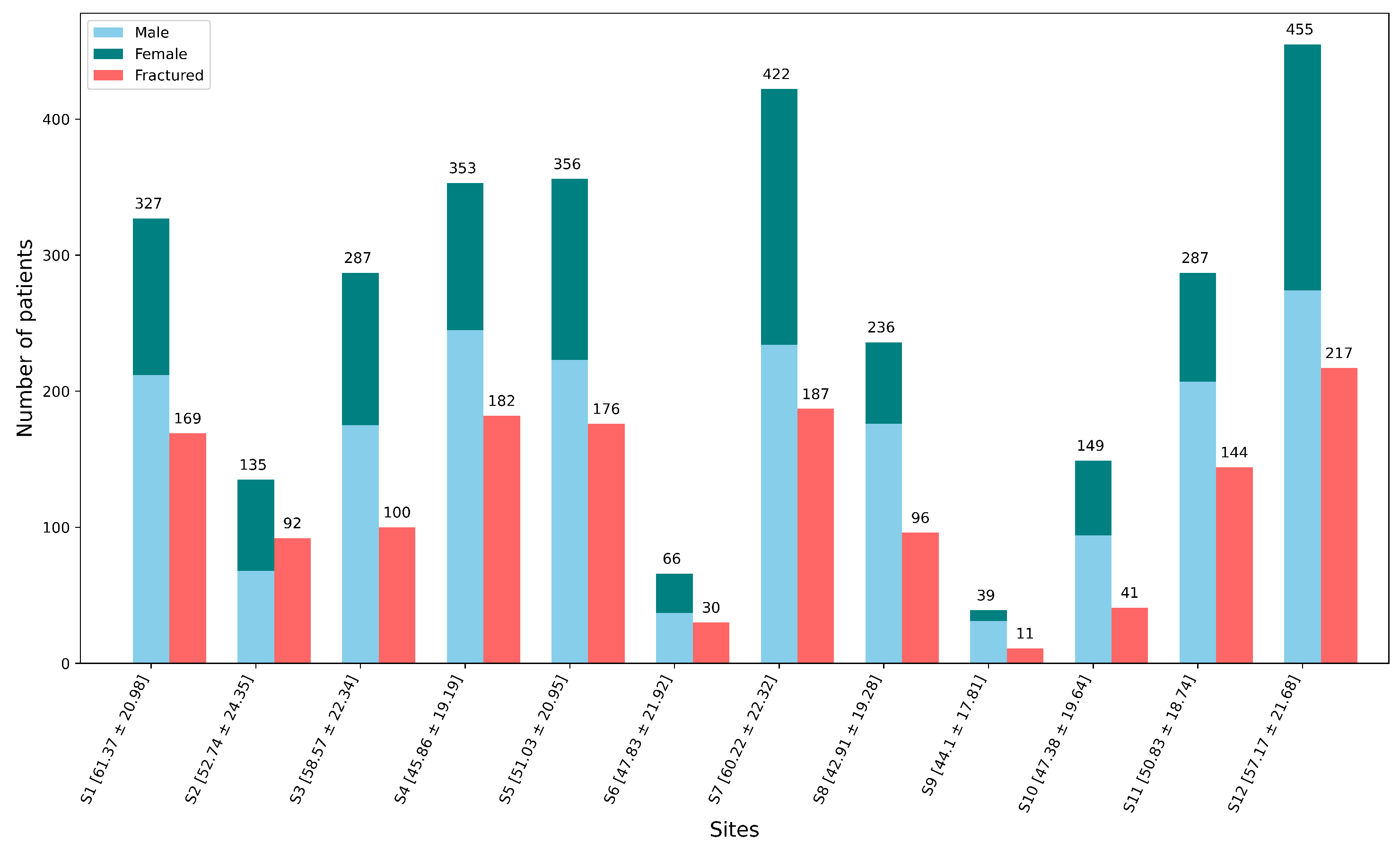
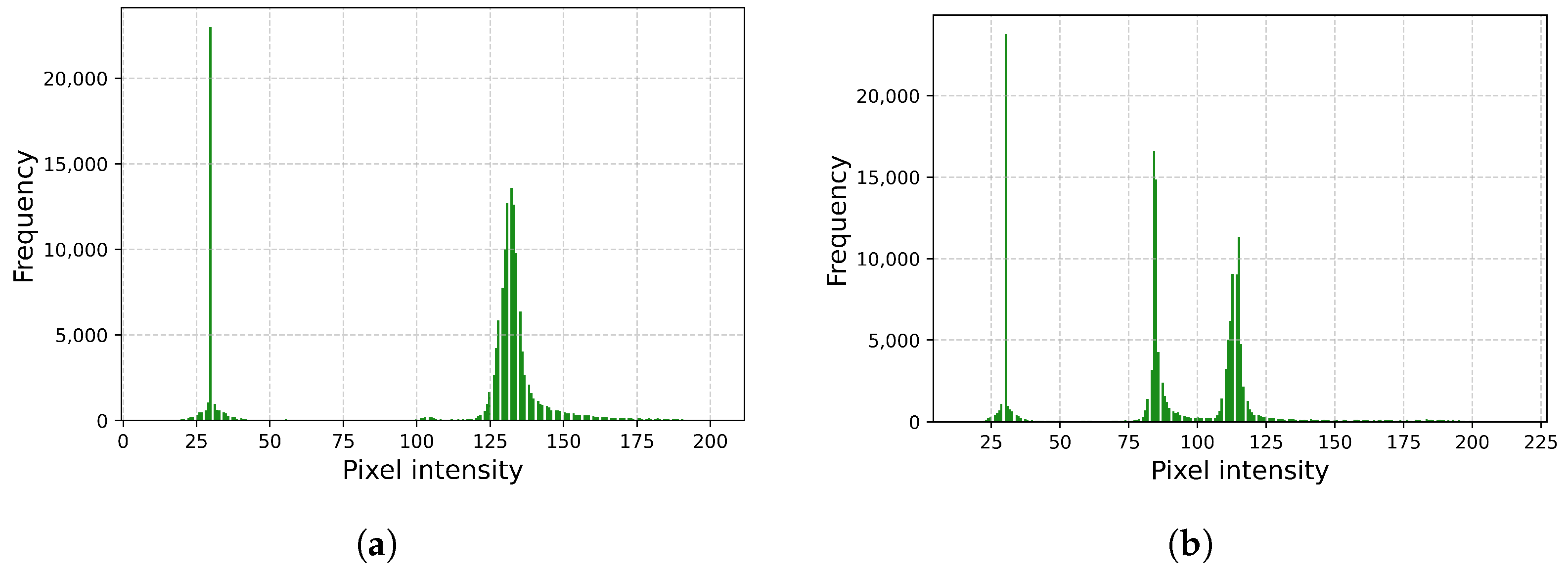
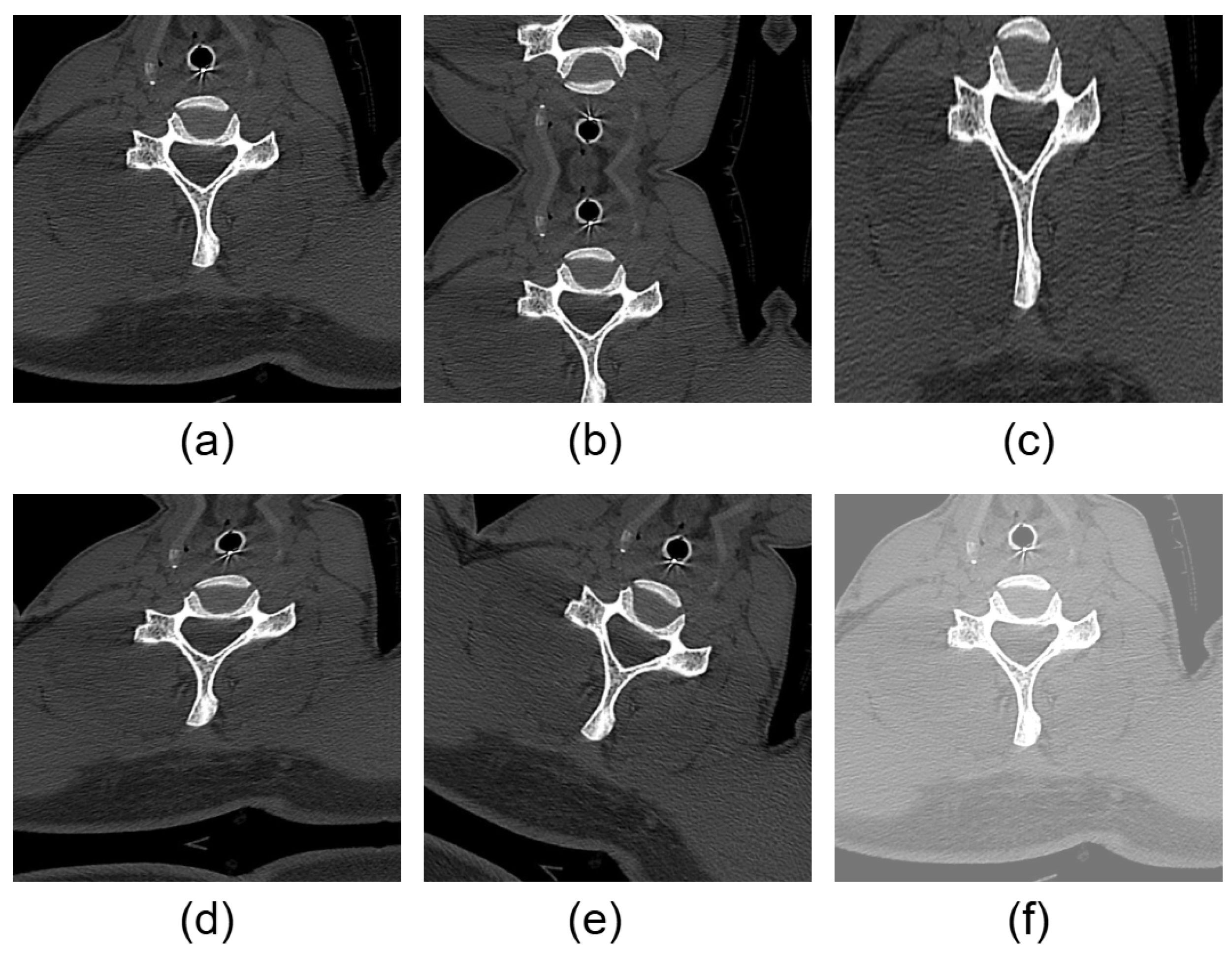
2.1. About Dataset and Its Preprocessing

The dataset used in this study is originally in digital imaging and communications in medicine (DICOM) format, and was obtained from an open source repository [25]. Figure 1 presents a bar plot of the data, collected from 12 independent sites ranging from ($S1$ to $S12$), which are represented by the X-axis, along with the mean and standard deviation (SD) of the ages of the patients for each site, whereas the Y-axis represents the number of patients. The first bar in each site indicates the total number of patients that underwent the CT scan, in which the number of male and female patients are represented by sky-blue and teal colors, respectively. The adjacent red bar highlights the number of patients with fractures. The present study utilizes a dataset comprising 2019 patients, yielding 15,123 CT images in the axial plane. The patients are classified into two categories, fracture and non-fracture. The number of images in the fracture and non-fracture classes is 7217 and 7906, respectively. The dataset, provided by the Radiological Society of North America (RSNA), contains images from multiple sites across nine countries and six continents, labeled by medical experts. The patient’s ages in each site are represented on the X-axis in Figure 1, which shows that the minimum age of the patients is 23.63 years ($S8$ location), and the maximum age 82.35 years ($S1$ location). It indicates the diversity of data in terms of age, demographics, and class distribution, which may help to improve the generalizability of the model.

The DICOM images can be enhanced by meticulously choosing the appropriate window width ($w_i$) and window center ($c_i$) [26]. The choice of appropriate $w_i$ and $c_i$ highlights the most relevant details, such as bone fractures, locations, and their extent. In the dataset used for this study, the Hounsfield unit (HU) range of CT images varies from −100 HU to 800 HU, where −100 and 800 represent the deepest black and the brightest pixels, respectively. Following some experiments with different values of $w_i$ and $c_i$, the values of $w_i$ and $c_i$ were selected to be 670 and 290, respectively, to highlight the vertebral bone structure and the soft tissues in the DICOM images. The DICOM format also contains patient metadata, which increase the file size and are irrelevant for base model training. So, after emphasizing the most significant details by choosing the appropriate $w_i$ and $c_i$, all the CT images are converted to JPG to train the models.

Pixel intensity versus frequency graphs plotted for a sample image from both the non-fracture and fracture classes are shown in Figure 2. Figure 2a is skewed toward higher intensity, indicating that the presence of any fracture in bone is less likely. In Figure 2b, the middle spike indicates that there is a gap in the bone since the pixel intensity range 70–105 corresponds to gray shed, and that indicates that possibly, a fracture in the bone is present.

2.2. Data Augmentation

The dataset has come from different picture archiving and communication systems (PACS), which typically are inconsistent with some noises, and there are different orientations and variations depending upon the image modalities. This may hinder the generalizability of the deep learning model. To address this issue, the training dataset is prepared by applying various data augmentation methods. Translation and scaling help the model generalize across slight positional shifts and variations in vertebra size that can occur in images as it is obtained from different PACS. Elastic transformation handles small deformations and replicates anatomical variations and minor deformations which may occur due to patient positioning during the scan. The rotation accounts for slight tilts and variations in the scan angles, and ensures that the model is not biased toward a fixed orientation. Lastly, contrast and brightness adjustment addresses the variations in light effect during scan to ensure the model remains invariant to contrast-related changes. A sample image from the non-fracture class along with the output of various symmetric and asymmetric augmentation strategies are displayed in Figure 3. The first image represents the original CT image from the non-fractured class, followed by the output of different operations, specifically, translation, zoom-in, elastic transformation, rotation, and contrast/ brightness adjustment, respectively.

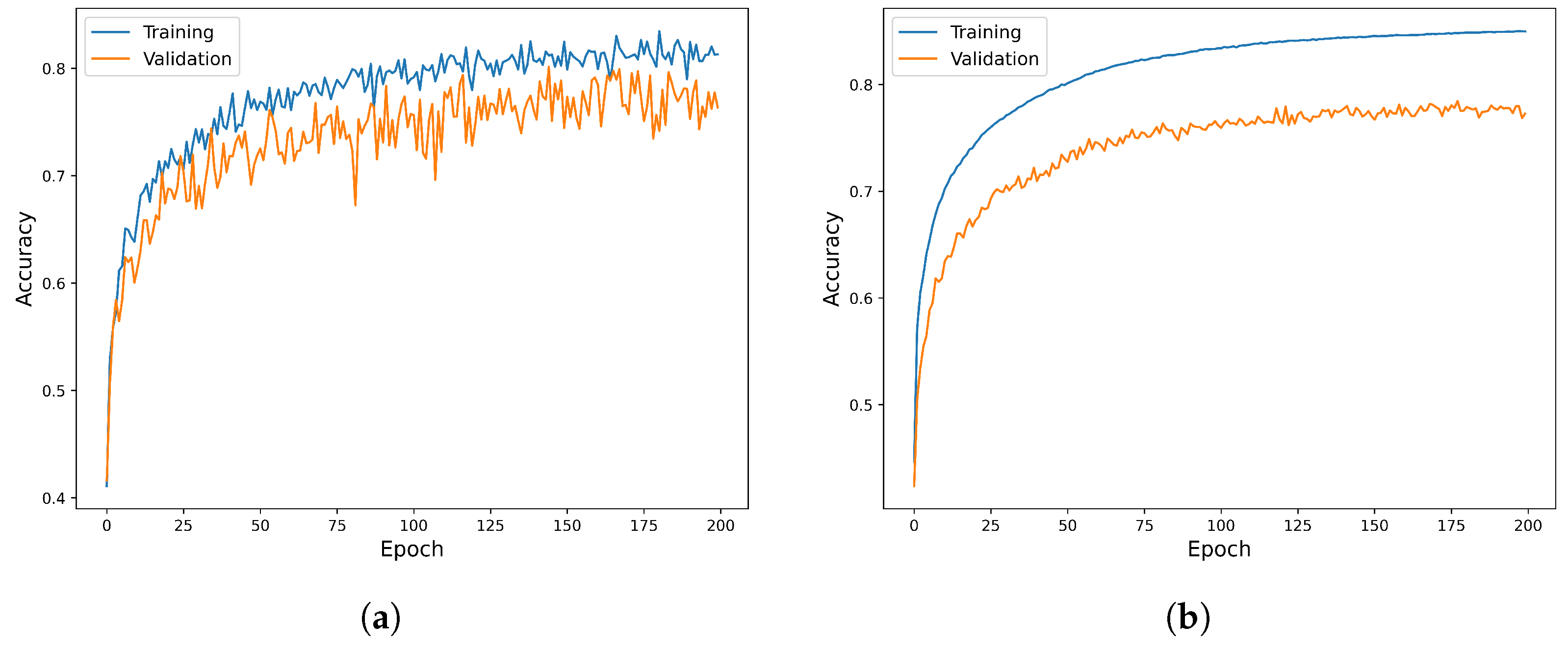
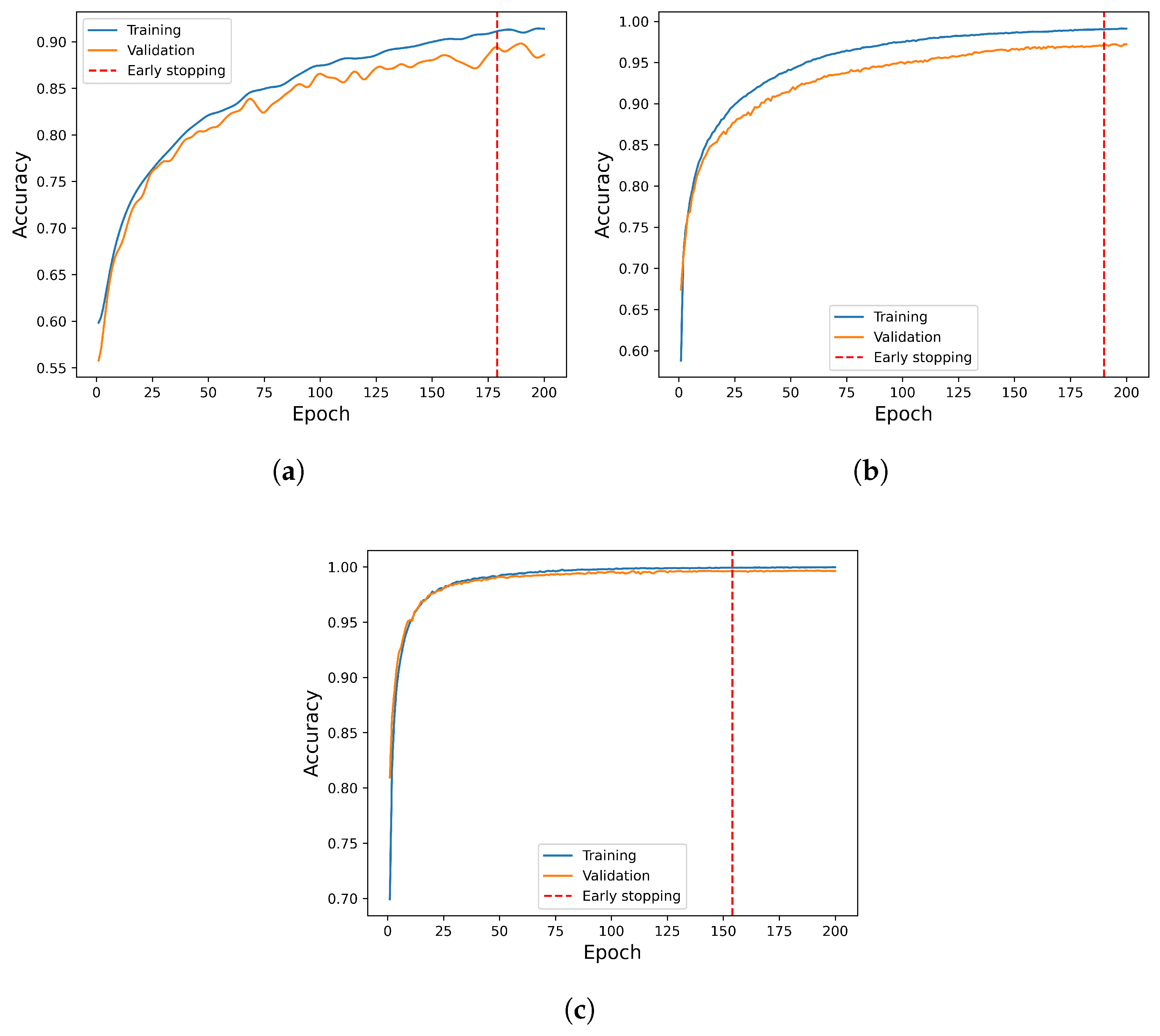
2.3. Base Models’ Training and Their Hyperparameter Optimization

As discussed in Section 1, ResNet, DenseNet, and EfficientNet are extremely successful in addressing many different problems related to medical imaging with CT data. However, their potential for addressing spine-related issues has been little explored. Motivated by the ensemble learning theory, which suggests using heterogeneous models to maximize diversity and improve generalization in stacking [27], and also given the recognized advantages in extracting different features, the models WideResNet-40 (WRN-40) [28], DenseNet-121 [29], and EfficientNet-B7 [30] are chosen as base models for the proposed methodology to detect C-spine vertebral fractures. These models have different architectures, depth, and feature extraction strategies, ensuring complementary learning. Additionally, they are computationally efficient and effectively alleviate the vanishing gradient problem using various strategies. ResNet-152 [31] and ResNet-200 [32] are also utilized to train on our dataset to validate the choice of base models. Both variants of ResNet are trained using the Adam optimizer, with a batch size of 32 and for 200 epochs. To avoid overfitting, L2 regularization is employed in both models during training. A similar hyperparameter setup, which is used for the chosen base models, is introduced in these two models. The training and validation accuracy patterns are shown in Figure 4a indicating significant fluctuations in ResNet-152, suggesting that the model is prone to underfitting and capturing noise rather than learning the underlying patterns in the data. In the case of ResNet-200, a significant gap is observed between the training and validation accuracy shown in Figure 4b, which demonstrates an overfitting issue. Additionally, the accuracy, specificity, sensitivity, and F1-score achieved by ResNet-152 are 62.9%, 58.37%, 61.09% and 59.72%, respectively. And, ResNet-200 achieved 64.17% accuracy, 56.02% specificity, 60.93% sensitivity, and 61.4% F1-score. These results are also illustrated in Section 3, which are not very encouraging, indicating that neither variant is a suitable candidate for a base learner. A brief overview of the base models along with their core components, and the training, as well as the fine-tuning of the hyperparameters, are explained below.

A multi-layered network is required to detect tiny features, including subtle textures, shapes, and structures, such as hairline fracture. And deeper ResNet, which did not show promising results, might encounter vanishing gradient problems. To address this, WideResNet, an improved version of ResNet was proposed by Zagoruyko et al., in which the number of filters per layer is increased. This reduced the need of the network to be deeper. The skip connection, shown in Figure 5a, is the core component of WRN-40 that improves feature flow and feature reuse across all layers by eliminating the vanishing gradient issue. The input X in Figure 5a is sent to $1\times 1$ convolution, which reduces the number of channels in the feature maps. Then, the output feature maps are fed into a $5\times 5$ convolution block, a larger filter, that extracts the features well, followed by a $1\times 1$ convolution, which restores the original channel dimension of the feature maps. The number of kernels in the $5\times 5$ convolution block is $16k$, where k represents the widening factor, and the base number of channels is 16. Choosing the value $k=4$, the number of kernels becomes 64 after widening.

Dense connection is the core component of DenseNet, it improves feature propagation and allows the reuse of features across the DenseNet network. The architecture of the first dense block of DenseNet-121 is shown in Figure 5b, which demonstrates that each convolution layer in the dense block receives feature maps from all preceding layers, helping the network to capture and utilize information from different levels of the model. DenseNet typically has fewer parameters than other deep CNN networks as it reuses the features across layers, resulting in a more efficient model.

EfficientNet scales the network width, depth, and resolution and balances them with the help of compound scaling, as discussed in [30]. In the present study, the EfficientNet-B7 variant is chosen, as it turns out to be more accurate than the other versions of EfficientNet. The mobile inverted bottleneck (MB) convolution block is the basic building block of EfficientNet-B7, which integrates the squeeze-and-excitation (SE) block with the inverted residual network, helping EfficientNet-B7 to emphasize the most relevant features. The schematic diagram of the MB convolution block is shown in Figure 5c.

The chosen three base learners, provided with pre-trained ImageNet [33] weights are further trained with the chosen CT dataset. The probabilities predicted by them will be used in the next level of the proposed ensemble model. For this, the dataset is split into training, validation, and test sets by patients in the ratio of 70%, 15%, and 15%, respectively. For training, the input images are resized into different dimensions as per the requirements of the base models. Therefore, all the training images are resized into $32\times 32$, $224\times 224$, and $256\times 256$ to feed into WRN-40, DenseNet-121, and EfficientNet-B7, respectively, followed by batch normalization and data augmentation.

To obtain the best possible combination of hyperparameters for all three base models, a grid search approach along with 5-fold CV is employed. The hyperparameters, their reference ranges, and the chosen values through the grid search and 5-fold CV are given in

Table 1. Experimental setup and chosen hyperparameters for base models.

Hyperparameter	Reference	Chosen Value
		WRN-40	DenseNet-121	EfficientNet-B7
Learning rate	[0.0001, 0.01]	0.001	0.0001	0.0001
Batch size	[16, 128]	32	32	32
Optimizer	-	Adam	SGD	Adam
Epoch	-	200	200	200
Model checkpoint	-	15 epoch	15 epoch	15 epoch
Dropout rate	[0, 0.6]	0.5	0.3	0.4
Weight decay	$[{10}^{-6},{10}^{-2}]$	${10}^{-4}$	${10}^{-4}$	${10}^{-5}$
Data augmentation	-	✔	✔	✔
Growth rate	[12, 48]	-	32	-
Compression factor	[0.1, 1.0]	-	0.5	-
Width coefficient	[1.0, 2.0]	-	-	1.5
Depth coefficient	[1.0, 3.0]	-	-	2.5

. The initial learning rates are chosen as small values for better convergence. The batch size and number of epochs for all three models are selected as 32 and 200, respectively. Moreover, regularization techniques, such as weight decay, along with appropriate dropout rate are applied to avoid overfitting issues, which are indicated in Table 1. The growth rate, which indicates the number of feature maps added per layer within each dense block, and the compression factor, which determines the size of the feature maps that need to be reduced in the transition block, are two important parameters of DenseNet-121. The width coefficient and depth coefficient, the two fundamental parameters of EfficientNet-B7, which are chosen to be $1.5$ and $2.5$, respectively, represent the extent of scaling.

As discussed in Section 2.1, the fracture class and the non-fracture class account for 47.72% and 52.27% of the total data, respectively, indicating the data are slightly imbalanced. To ensure that the model gives equal importance to both the classes during training, weighted binary cross-entropy (WBCE) is found suitable and chosen as the loss function, which is expressed as follows:

$$L=-{\displaystyle \frac{1}{N}}\sum _{i=1}^N\left({\alpha }_1{y}_{i}log\left({\widehat{y}}_i\right)+{\alpha }_0(1-y_i)log(1-{\widehat{y}}_i)\right)$$

(1)

where $y_i$ and ${\widehat{y}}_i$ represent the true and predicted value, respectively, and ${\alpha }_j$ represent the weights for the class $j=0,1$, which are obtained using the formula given below,

$${\alpha }_j={\displaystyle \frac{N}{2n_j}}$$

Here, N is the total number of samples, and $n_j$ denotes the total number of samples in class j.

The 5-fold CV also validates and ensures that the base models are not biased to any particular fold of training data. The statistical insights of the base learners using 5-fold CV are displayed in Figure 6 and their performance on the validation set is presented in

Table 2. Performance metrics across 5-Fold CV for base learners.

Model	Metric	Training	Validation
WRN-40	Acc	$88.29\pm 2.18$	$84.3\pm 2.61$
	Spec	$88.1\pm 3.64$	$85.2\pm 3.19$
	Sens	$86.12\pm 2.5$	$80.1\pm 3.09$
	F1	$86.4\pm 2.31$	$82.3\pm 3.03$
DenseNet-121	Acc	$89.17\pm 1.54$	$86.2\pm 3.34$
	Spec	$87.4\pm 2.82$	$82.6\pm 3.73$
	Sens	$91.3\pm 2.72$	$89.6\pm 2.53$
	F1	$89.32\pm 3.14$	$86\pm 3.82$
EfficientNet-B7	Acc	$94.17\pm 2.17$	$90.26\pm 1.78$
	Spec	$92.7\pm 2.93$	$88.14\pm 1.54$
	Sens	$93.24\pm 2.03$	$91.8\pm 2.08$
	F1	$93.8\pm 2.15$	$89.8\pm 2.07$

. From the box plots of each base model, it is evident that all four performance metrics vary in a narrow range, whose values are also presented in Table 2 in the form of mean ± SD.

To gain insights into the decision-making process of our base models and to understand which feature of the CT image contributes more for making predictions, this study utilized the SHapley Additive exPlanations (SHAP) technique [34], which is demonstrated in Figure 7. The SHAP values, represented by color gradients ranging from dark blue (highest negative contribution) to dark pink (highest positive contribution) via white (no contribution), illustrate the contribution of each feature to the model’s prediction. Furthermore, a small fracture area highlighted in a green rectangular box is zoomed in and displayed in the adjacent column for enhanced visualization. The first, second, and third rows display the SHAP results obtained from WRN-40, DenseNet-121, and EfficientNet-B7, respectively. It can also be observed that, for a test image belonging to a fracture class, the output in the non-fracture SHAP explanation column is obtained with blue, indicating false prediction, while the fracture SHAP explanation column is coded with pink, indicating correct prediction. Conversely, when the test image belongs to the non-fracture class, the color-coding is as follows: the non-fracture SHAP explanation column is colored with pink, indicating correct prediction, and the blue will appear in the fracture SHAP explanation column, suggesting false prediction.

Feature maps obtained from the second convolutional layer of the base models and the class activation maps (CAM) from their last convolutional layers are displayed in Figure 8. The leftmost image in Figure 8 represents a randomly chosen fractured-class image from the test set, which is used to visualize how well the base learners make predictions on unseen data. The light green arrows in the chosen sample image indicate two fractured regions. The upper three images in Figure 8 illustrate the feature maps extracted from the second convolutional layer of WRN-40, DenseNet-121, and EfficientNet-B7, showing that they have effectively captured low-level features, such as edges, outlines, and the texture of the object of interest, i.e, vertebral bones. If an image contains even a single fracture, it is classified as fractured class. The bottom row in Figure 8 represents the CAMs generated by the last convolutional layer of the base models, which are generated using Grad-CAM [35]. The output of WRN-40 highlights one fracture region, while DenseNet-121’s CAM emphasizes the other. However, EfficientNet-B7 is able to identify both the fractures, though the lower fracture region is not prominently learned. This heatmap study justifies the choice of the three base models and motivates combining them to propose an ensemble method, which can achieve higher performance than that of the individual base models, as discussed in the next section.

2.4. Proposed Method

Combining the predictions obtained from various suitable models appropriately, also termed ensemble learning, has proven to be an effective approach for improving prediction accuracy [36]. It aims to achieve more reliable and accurate prediction than that of a single model. Bagging and boosting are two popular traditional ensemble learning approaches, which are found to be very effective in many applications [37]. Stacking is also a widely used ensemble approach introduced by [38]. Employing different models as base learners is always preferable, as each learner tries to learn diverse features during the training phase. In this study, three different models are chosen as base learners, and therefore, the stacking strategy which is suitable to combine the predictions is used.

The primary concern with existing ensemble methods is that they give equal importance to all the base models, or the weights are assigned based on some predefined function [39]. However, all the models may not perform alike on the same dataset. Therefore, combining the performances of the base models has to be performed in a meaningful way. The base models that are chosen to obtain the prediction are not guaranteed as the best models, as there could be other possible models that may give different predictions for the same data. The typical ensemble learning approach that combines the model’s prediction ignores this uncertainty about the base models. To address this, we introduce a Bayesian probability-based novel ensemble learning approach for effectively combining the base model’s predictions. Our approach handles the aforementioned issue by considering the uncertainty in the model and allows us to assign different weights to the models based on their performance. The diagram shown in Figure 9 demonstrates the workflow of the proposed method where, $f_1$, $f_2$, and $f_3$ represent the prediction obtained from WRN-40, DenseNet-121, and EfficientNet-B7. Then, performance metrics are calculated for the base models on the validation dataset, which are utilized to obtain their prior probabilities. In the next step, the posterior probability is calculated using the maximum likelihood estimation (MLE) method. Based on these findings, finally, the weights of the base learners are obtained using Bayes theorem, which are the key findings in this study, and are used to combine the predictions of the three fine-tuned base models. The procedure of the proposed approach is outlined in Algorithm 1, which is discussed below in detail.

Algorithm 1: Proposed ensemble learning algorithm

The dataset $D=[y_{{\mathrm{obs}}_1},y_{{\mathrm{obs}}_2},\dots ,y_{{\mathrm{obs}}_T}]$ comprises the true labels of the images in the training set, where T is the total number of images. Let the outcome (probability) of each base model for a given image, belonging to the fracture or non-fracture class, be represented by $y_i$, $i=0,1$. The three base models, WRN-40, DenseNet-121, and EfficientNet-B7 are denoted by $M_1$, $M_2$ and $M_3$, respectively. Suppose the predictions of $M_1$, $M_2$, and $M_3$ for all the T images are represented by $f_1,f_2$ and $f_3$, respectively. Therefore, each $f_m,m=1,2,3$ contains a random sequence of probability values $y_i$, of length T. Then, the intuition is that $M_1$ might be excellent in predicting certain patterns in the data, $M_2$ could handle other patterns that are missed by $M_1$, and $M_3$ may capture some unique information missed by the previous two. Therefore, the posterior distribution of the variable y which assumes the values $y_i$, given the dataset D, is represented as,

$$\begin{array}{c}\hfill p\left(y\right|D)=\sum _{m=1}^{3}p\left(y\right|f_m,D)p\left(f_m\right|D)\end{array}$$

(2)

where $p\left(y\right|f_m,D)$ is the probability of y given the $m^{th}$ model prediction and data D, which also represents the actual prediction obtained by the $m^{th}$ model. And, $p\left(f_m\right|D)$ is the posterior probability of the $m^{th}$ model given the data D, which also acts as the weight assigned to the $m^{th}$ model. If the $m^{th}$ model performs well on the validation set, then the value of $p\left(f_m\right|D)$ will also be higher [40].

The posterior distribution $p\left(f_m\right|D)$ can also be expressed based on Bayes’ theorem as,

$$\begin{array}{c}\hfill p\left(f_m\right|D)={\displaystyle \frac{p\left(D\right|f_m)\pi \left(f_m\right)}{{\sum }_{j=1}^{3}p\left(D\right|f_j)\pi \left(f_j\right)}},m=1,2,3\end{array}$$

(3)

where $p\left(D\right|f_m)$ represents the likelihood of the data given prediction $f_m$ and $\pi \left(f_m\right)$ is the prior probability of the $m^{th}$ model.

As per the central limit theorem, it is assumed that the combined predicted distribution, $\widehat{y}$, from all three models follows a normal distribution with mean ${\mu }_m$ and SD ${\sigma }_m$, i.e., $\widehat{y}\sim \mathcal{N}({\mu }_m,{\sigma }_m^2)$. The probability distribution function (PDF) of $\widehat{y}$ is expressed as

$$\begin{array}{c}\hfill f\left(\widehat{y}\right)={\displaystyle \frac{1}{{\sigma }_m\sqrt{2\pi }}}exp\left(-{\displaystyle \frac{1}{2}}{\left({\displaystyle \frac{\widehat{y}-{\mu }_m}{{\sigma }_m}}\right)}^2\right)\end{array}$$

(4)

The likelihood $p\left(D\right|f_m)$ in Equation (3) can also be expressed as $f(\widehat{y}\mid {\theta }_m)$, where ${\theta }_m=({\mu }_m,{\sigma }_m^2)$. Subsequently, the parameters of Equation (4) are estimated using the maximum MLE [41]. Let the estimated parameters be denoted as $\widehat{\theta }=({\widehat{\mu }}_m,{\widehat{\sigma }}_m^2)$, which are expressed below as

$$\begin{array}{c}\hfill {\widehat{\mu }}_m={\displaystyle \frac{1}{T}}\sum _{i=1}^T{\widehat{y}}_i\end{array}$$

$$\begin{array}{c}\hfill {\widehat{\sigma }}_m=\sqrt{{\displaystyle \frac{1}{T}}\sum _{i=1}^T{({\widehat{y}}_i-{\widehat{\mu }}_m)}^2}\end{array}$$

As the prior probability $\pi \left(f_m\right)$ for the $m^{th}$ model is directly proportional to the performance of that model across all metrics, it is arguably relevant to estimate as follows:

$$\begin{array}{c}\hfill \pi \left(f_m\right)={\displaystyle \frac{Ac{c}_m+Spe{c}_m+Sen{s}_m+F{1}_m}{{\sum }_{l=1}^3(Ac{c}_l+Spe{c}_l+Sen{s}_l+F{1}_l)}}\end{array}$$

(5)

where $Ac{c}_m$, $Spe{c}_m$, $Sen{s}_m$ and $F{1}_m$ represent, respectively, the accuracy, specificity, sensitivity, and F1-score of the $m^{th}$ base model. Equation (5) shows that the prior probability $\pi \left(f_m\right)$ is estimated as the normalized performance of all the individual base models. Also, it indicates that, while the performance of a model increases, the prior probability of that particular model is improved.

Now, the estimated values of $p\left(D\right|f_m)$ and $\pi \left(f_m\right)$ obtained for all three base learners are substituted in Equation (3). The values of $p\left(f_1\right|D)$, $p\left(f_2\right|D)$ and $p\left(f_3\right|D)$, which are denoted as $w_1$, $w_2$, and $w_3$, are the weights of WRN-40, DenseNet-121, and EfficientNet- B7, respectively.

To obtain the ensemble prediction, the weights are multiplied by the corresponding model’s prediction and summing them across all the models as follows:

$$\begin{array}{c}\hfill E_i^n=\sum _{m=1}^3{w}_m{p}_{mi}^{n}i=0,1,m=1,2,3\end{array}$$

(6)

where $E_i^n$ represents the ensemble probability prediction for the $n^{th}$ test image of $i^{th}$ class. And, $p_{mi}^n$ represents the probability predicted by the $m^{th}$ base model for the $n^{th}$ test image and $i^{th}$ class.

Finally, using the ensemble probability obtained in Equation (6), the updated predicted class $C_n$ for the $n^{th}$ test image is obtained as follows:

$$\begin{array}{c}\hfill C_n=arg\underset{i\in \{0,1\}}{max}\left(E_i^n\right)\end{array}$$

The final predicted class, using the proposed method, is then compared with the true label to generate the confusion matrix. And, based on the confusion matrix, the performance metrics accuracy, sensitivity, specificity, and F1-score are calculated.

To investigate the impact of noise on the prediction accuracy, we selected a test image sample and created two versions, one with added noise and another in its original form, and generated heatmaps for both images. The first row in Figure 10 shows the original CT image (without noise) and its heatmaps obtained from WRN-40, DenseNet-121, and EfficientNet-B7, respectively. The subsequent two rows demonstrate the noisy images with different noise levels and their heatmaps. The noisy images are generated by introducing moderate and high Gaussian noise with SD $\sigma$ = 25 and SD $\sigma$ = 50, respectively, in the chosen sample image. The feature activation heatmaps are generated using Grad-CAM from the last convolutional layer of all the three base models separately. The heatmaps generated by the base models reveal a consistent focus on the bone regions of the vertebrae, which are the most prominent feature. When moderate noise is introduced, the base models remain effective in concentrating on the bone structure, with minimal impact from the noise. However, as evident in the last row of Figure 10, when the high noise is introduced, the models’ confidence in their predictions decreases. The reason is that the vertebral bone structure becomes less apparent due to noise, making it difficult for the models to correctly identify the prominent features. This analysis highlights the robustness of the base models, which have learned strong feature representations that enable them to withstand moderate levels of noise. Nevertheless, it also highlights the limitations of these models when confronted with high levels of noise.

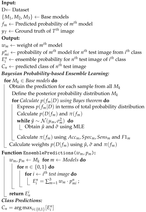
2.5. Experimental Setup

The experiments are carried out on a workstation embedded with a Tesla V100 GPU and CentOS Linux version 8.5.2111. The system is configured as an Intel(R) Xeon(R) Gold 6254, with a clock speed of 3.1 GHz and 32 GB RAM. The entire workflow is implemented in PyTorch version 1.9.0 with CUDA version 11.0 in the backend and Python 3.8.3 using a random seed 36. The time taken to train the WRN-40, DenseNet-121, and EfficientNet-B7 is approximately 3.58, 4.16, and 6.25 h, respectively. Following training, the inference time that a single model takes is 1.12 s, and therefore, the total inference time for all three base models is approximately 2.1 h. The time required to ensemble all the predictions by the proposed method is about 1.7 min (0.028 h). Therefore, the total runtime, including the inference and ensembling time, of the proposed approach is 16.11 h on the aforementioned workstation’s specification.

3. Results

In this section, the results of the proposed model are discussed and compared with the results of each base model. Furthermore, to validate the efficiency of the proposed method, the results obtained from traditional ensemble techniques and closely related existing works in the literature are compared and analyzed separately in this section.

3.1. Evaluation Metrics

This study utilizes a confusion matrix to evaluate the proposed model. Accuracy (Acc), specificity (Spec), sensitivity (Sens), and F1-score (F1) are chosen to assess the model performance. In the present work, sensitivity and specificity are emphasized as they together provide balanced evaluations. High sensitivity ensures fracture cases are detected correctly, and high specificity reveals that non-fractured cases are correctly classified. The formulae for the performance metrics are given below:

$$\begin{array}{cc}\hfill \left(\mathrm{i}\right)& Acc={\displaystyle \frac{TP+TN}{TP+FP+TN+FN}}\hfill \\ \hfill \left(\mathrm{ii}\right)& Spec={\displaystyle \frac{TN}{TN+FP}}\hfill \\ \hfill \left(\mathrm{iii}\right)& Sens={\displaystyle \frac{TP}{TP+FN}}\hfill \\ \hfill \left(\mathrm{iv}\right)& F1={\displaystyle \frac{2\times Precision\times Sens}{Precision+Sens}}\hfill \end{array}$$

Here, True Positive (TP), True Negative (TN), False Positive (FP), and False Negative (FN) are the entries of the confusion matrix. However, precision may not be a suitable evaluation measure in our context, since high precision may sometimes fail to detect the fracture cases. But, as it is required to calculate the F1-score, the following formula is used to calculate the precision:

$$\begin{array}{cc}\hfill \left(\mathrm{v}\right)& Precision={\displaystyle \frac{TP}{TP+FP}}\hfill \end{array}$$

3.2. Analysis of Results Obtained from Conventional Ensemble Approaches

To justify the effectiveness of the proposed ensemble approach, some popular conventional ensemble learning approaches, such as majority voting [42], average probability [43], and weighted average probability (WAP) [44], are also implemented on our data (RSNA-2022) to combine the predictions from the chosen base learners. Each base model predicts a class for an image in majority voting ensemble learning, and the final class is determined by the maximum number of votes obtained from each base model. This approach’s primary drawback is that it treats all base models equally, even if one model is more confident about its prediction than another. In the average probability approach, a predicted probability is assigned to each class by all base models. These probabilities are then averaged over all models, and the final prediction is made for the class with the highest average probability. The major drawback of this approach is the final prediction becomes weak after averaging. For example, consider two models predicting the same image as fractured, but with vastly different probabilities, 0.8 and 0.2. Averaging these predictions would result in a probability of 0.5, potentially diluting the strength of the final prediction. In WAP ensemble learning, the predicted probability obtained from each base learner is considered as a weight of the respective model, and the final class is obtained as a weighted average of the predicted probabilities. Although this method is better than the previous two, the weight calculation often depends on the performance on validation data, making it less adaptable to unseen data. The results obtained from these traditional approaches are compared with the proposed model, which is listed in

Table 3. Comparison of results obtained from proposed method with traditional ensemble learning methods.

Ensemble Method	Acc (%)	Spec (%)	Sens (%)	F1 (%)
Majority voting	$89.17$	$83.2$	$88.05$	$85.03$
Average probability	$91.27$	$90.06$	$91.1$	$90.06$
WAP	$92.3$	$90.56$	$92.72$	$91.11$
Proposed	$\mathbf{94}.\mathbf{62}$	$\mathbf{93}.\mathbf{51}$	$\mathbf{95}.\mathbf{29}$	$\mathbf{93}.\mathbf{16}$

.

The proposed method outperforms all the existing conventional ensemble approaches. Although the WAP method performs well, our method yields a slight improvement over WAP across all the performance measures. The weights in the WAP are calculated based on a chosen function. However, in the proposed probabilistic-based ensemble approach, the weights are calculated based on the Bayesian framework, which yields more accurate predictions.

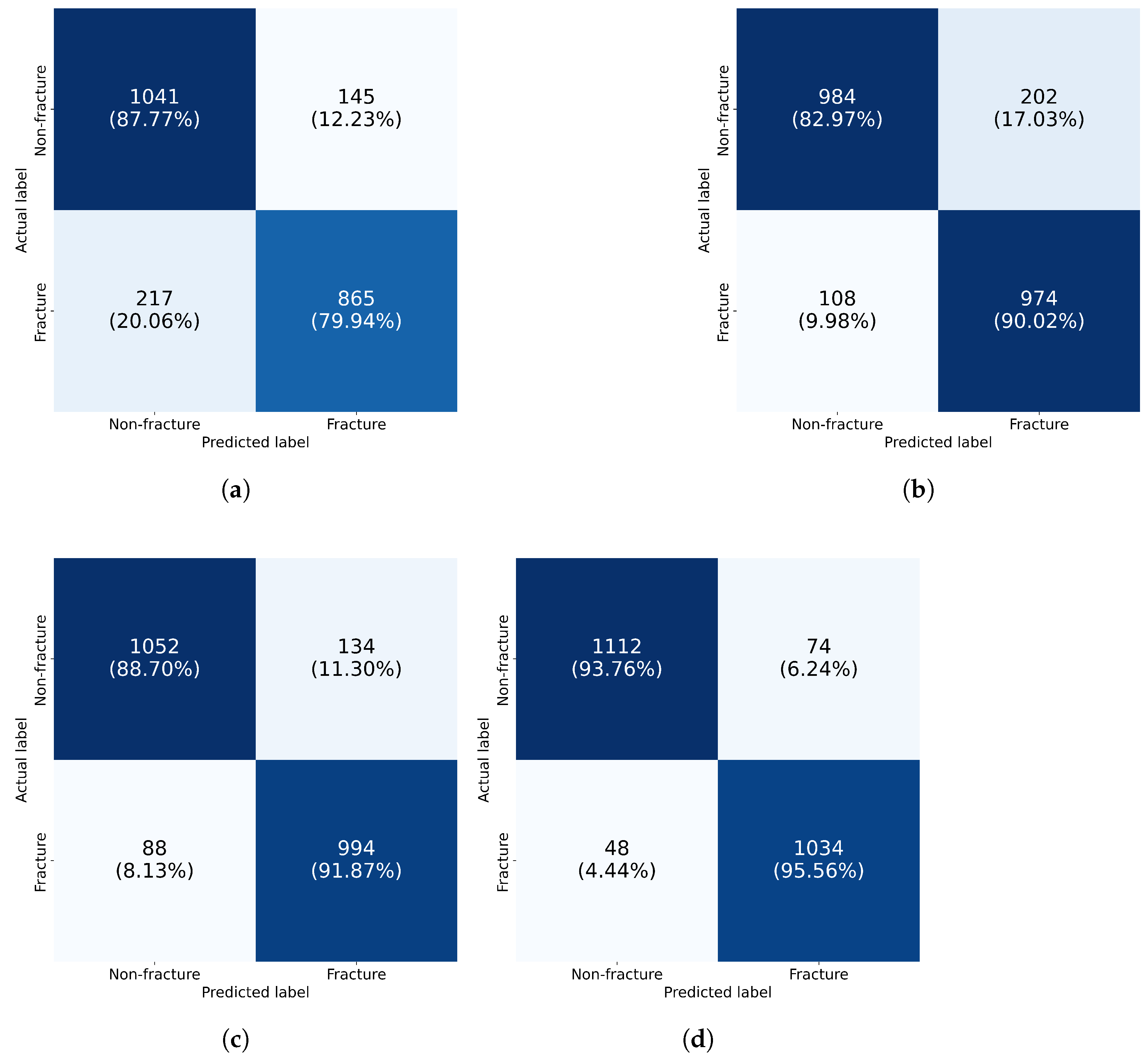
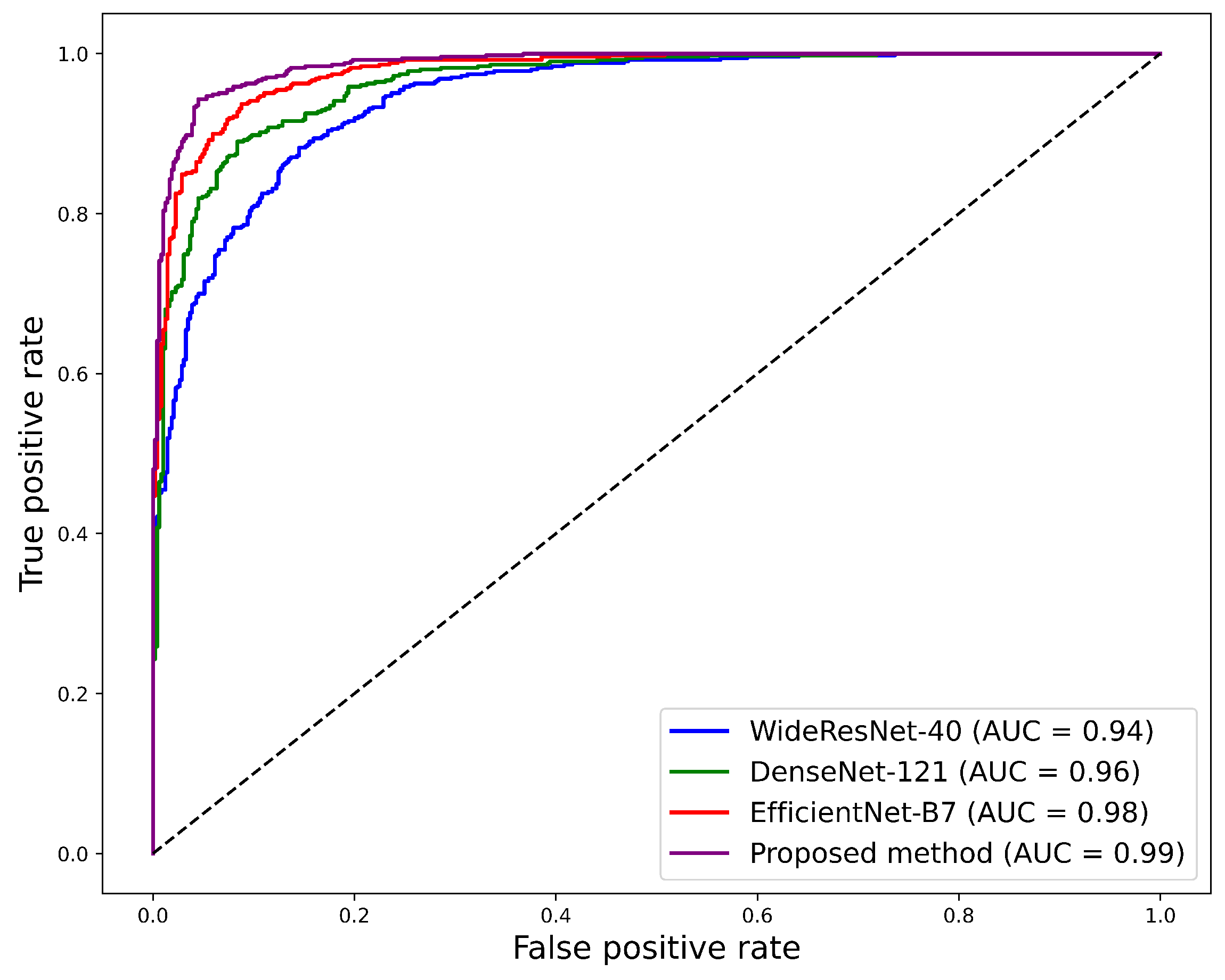
3.3. Performance Analysis of Individual Models and Proposed Ensemble Method

The training and validation accuracy curves for each base model are displayed in Figure 11. The dotted red vertical lines in Figure 11 represent the best validation accuracy for each model, for which the checkpoints are saved and used to obtain the prediction result. The test accuracies for WRN-40, DenseNet-121, EfficientNet-B7, ResNet-152, and ResNet-200 are found as 85.4%, 88.43%, 91.21%, 62.9% and 64.17%, respectively, as given in

Table 4. Analysis of results obtained from the individual CNNs and the proposed model.

Model	Acc (%)	Spec (%)	Sens (%)	F1 (%)	AUC (%)
WRN-40	$85.4$	$86.6$	$81.02$	$82.72$	$94.00$
DenseNet-121	$88.43$	$84.2$	$90.81$	$86.38$	$96.00$
EfficientNet-B7	$91.21$	$88.42$	$92.03$	$89.19$	$98.00$
ResNet-152	$62.9$	$58.37$	$61.09$	$59.72$	$87.2$
ResNet-200	$64.17$	$56.02$	$60.93$	$61.4$	$85.06$
Proposed	$\mathbf{94}.\mathbf{62}$	$\mathbf{93}.\mathbf{51}$	$\mathbf{95}.\mathbf{29}$	$\mathbf{93}.\mathbf{16}$	$\mathbf{99}.\mathbf{00}$

, whereas, for the proposed approach, it is 94.62%, which is superior to all the base models.

It can be observed from Table 4 that EfficientNet-B7 shows better performance compared to ResNet-152, ResNet-200, WRN-40, and DenseNet-121. However, the proposed method outperforms all individual base classifiers in terms of accuracy, specificity, sensitivity, and F1-score with 94.62%, 93.51%, 95.29%, and 93.16%, respectively. The confusion matrices shown in Figure 12 provide more insight into the model’s performance. The confusion matrix obtained from the proposed method demonstrates excellent performance with the best TP and TN, values along with the least FP and FN values compared to the base models. The receiver operating characteristic (ROC) curve in Figure 13 displays the area under the curve (AUC), which demonstrates the base models’ and proposed model’s ability to classify the fracture and non-fracture classes correctly. The proposed model achieves an AUC score of 99%, the highest of all.

3.4. Comparison with Other Existing Works

In this section, the results obtained from the proposed method are compared with existing work on VF detection found in the literature and are listed in

Table 5. Comparison of the proposed method with the other vertebral fracture detection models.

Existing Method	Acc (%)	Spec (%)	Sens (%)	F1 (%)	AUC (%)
Paik et al. [15]	$80.4$	$81.6$	$78.7$	$83.5$	−
Xu et al. [17]	$82.9$	$87.2$	$74.3$	$75.6$	$73.4$
Iyer et al. [16]	$86.67$	$84.2$	$88.13$	$87.04$	−
Small et al. [14]	92	$\mathbf{97}$	76	−	−
Chen et al. [18]	$73.59$	$73.02$	$73.81$	−	72
Chen et al. [19]	74	68	80	−	89
Ono et al. [20]	89	92	83	−	$87.6$
Nicolaes et al. [21]	93	93	94	−	94
Kojok et al. [22]	89	−	−	90	−
Guenoun et al. [23]	92	$91.7$	$92.3$	−	−
Proposed model	$\mathbf{94}.\mathbf{62}$	$93.51$	$\mathbf{95}.\mathbf{29}$	$\mathbf{93}.\mathbf{16}$	99

. The study by Small et al. [14] shows the best result in terms of specificity; however, its sensitivity lags by a large margin of 19.29%, and the accuracy also falls behind by 2.62% compared to those of the proposed model. The work proposed by Guenoun et al. [23] demonstrated excellent results and obtained performance measures near to our model, but it is lagging with a margin of 2.62%, 1.81% and 2.99% in terms of accuracy, specificity, and sensitivity, respectively. In another study [21], Nicolaes et al. showed the best result for VF detection; their result is very close to our study, with only slight differences of 1.62%, 0.51%, 1.29% in terms of accuracy, specificity, and sensitivity. However, their AUC score straggles by 5%, which is one of the critical measures of a model’s classification capabilities. Moreover, the study was conducted using a small set of data with patients age over 50 years, which may affect the model’s generalizability. The work by Iyer et al. [16] showed balanced results on all four performance metrics, but its accuracy lags by 7.95% compared to the proposed model. Overall, the proposed work demonstrates superior performance over all the methods compared in terms of accuracy, sensitivity, and F1-score, which indicates that our model is robust and accurate.

4. Conclusions

Identifying a small hairline fracture in a CT scan of a spine injury is challenging, and the risk of misclassification is higher. Our work focused on detecting the fractures in C-spine vertebrae using CT scans. It aimed to assist medical professionals in further treatment planning. Our approach utilized three CNNs as a base model and fused their prediction using a Bayesian-based probabilistic-ensemble learning approach. The objective of the proposed method was to improve the overall classification result. To accomplish this task, preprocessing steps, including handling the DICOM images and data augmentation, were performed; after that, base models were trained and fine-tuned using hyperparameter optimization and a 5-fold CV strategy. To validate the effectiveness of the proposed model, conventional ensemble techniques were also implemented with our dataset to combine the predictions from the base models, and the results were compared. Finally, it was observed that the proposed model yielded the best result in terms of accuracy, specificity, sensitivity, and F1-score. Since this work was performed on a diverse dataset obtained from various sites/modalities, it also turned out that the proposed model was more generalized, enabling potential integration with clinical use following expert radiologists’ verification. The proposed method may have vast potential for multidisciplinary applications, including, but not limited to, brain tumor detection, lung disease diagnosis, plant disease detection, and histopathology image analysis.

Although the proposed model showed excellent results, it also possesses some limitations. The results obtained by the proposed model are promising; however, clinical validation is a logical next step to further confirm its efficacy. Moreover, the computational complexity of our approach, although higher than that of a single model, is a worthwhile trade-off for the improved performance and robustness. Future research directions include exploring attention-based models to reduce computational costs and integrating our model into clinical workflows to enhance practical applicability. The proposed framework is accurate in distinguishing the fracture and the non-fracture vertebrae; however, the object detection models, like Faster R-CNN and Mask R-CNN, can be beneficial in localizing the fracture to identify the exact location of the injury. In addition, this study was validated on a robust dataset, where the ground truth was established by multiple experts from various countries. Although this multi-expert approach strengthens the study’s foundation, it also introduces potential inter-observer variability among the radiologists. To address this, future collaborations with medical experts will be invaluable in assessing consistency and enhancing the model’s generalizability. Furthermore, despite the success of ensemble learning, it is harder to visualize and interpret the features, since we cannot explicitly provide the feature activation maps obtained from the proposed method as the fusion of the results of the base learners is performed at the decision level. As CT scans provide volumetric data, performing a 2D CNN may distinguish the fractured image from non-fractured, but it is difficult to determine the extent of injury. An essential future area for study is the clinical validation of the proposed model, which is a crucial next step, offering a promising avenue for future research. In addition, to detect the fracture extent and exact slice in volumetric CT scans, integrating the spatial attention and channel attention module (CAM) in 3D CNN may help to identify the exact fracture region more efficiently by assigning a higher weight to the injured area during training. Furthermore, the combination of spatial attention and CAM may be more effective as spatial attention focuses more on the region of interest (fractured area), whereas CAM highlights the channel that carries the most important features.

References

1. Wallace, A.; Hillen, T.; Friedman, M.; Zohny, Z.; Stephens, B.; Greco, S.; Talcott, M.; Jennings, J. Percutaneous spinal ablation in a sheep model: Protective capacity of an intact cortex, correlation of ablation parameters with ablation zone size, and correlation of postablation MRI and pathologic findings. Am. J. Neuroradiol. 2017, 38, 1653–1659. [Google Scholar] [CrossRef] [PubMed]
2. Zanza, C.; Tornatore, G.; Naturale, C.; Longhitano, Y.; Saviano, A.; Piccioni, A.; Maiese, A.; Ferrara, M.; Volonnino, G.; Bertozzi, G.; et al. Cervical spine injury: Clinical and medico-legal overview. Radiol. Med. 2023, 128, 103–112. [Google Scholar] [CrossRef] [PubMed]
3. Dreizin, D.; Letzing, M.; Sliker, C.W.; Chokshi, F.H.; Bodanapally, U.; Mirvis, S.E.; Quencer, R.M.; Munera, F. Multidetector CT of blunt cervical spine trauma in adults. Radiographics 2014, 34, 1842–1865. [Google Scholar] [CrossRef] [PubMed]
4. Karlsson, A.K. Overview: Autonomic dysfunction in spinal cord injury: Clinical presentation of symptoms and signs. Prog. Brain Res. 2006, 152, 1–8. [Google Scholar]
5. Hamid, R.; Averbeck, M.A.; Chiang, H.; Garcia, A.; Al Mousa, R.T.; Oh, S.J.; Patel, A.; Plata, M.; Del Popolo, G. Epidemiology and pathophysiology of neurogenic bladder after spinal cord injury. World J. Urol. 2018, 36, 1517–1527. [Google Scholar] [CrossRef]
6. Stiller, W. Basics of iterative reconstruction methods in computed tomography: A vendor-independent overview. Eur. J. Radiol. 2018, 109, 147–154. [Google Scholar] [CrossRef]
7. Argyros, I.K. The Theory and Applications of Iteration Methods; CRC Press: Boca Raton, FL, USA, 2022. [Google Scholar]
8. Bate, I.; Murugan, M.; George, S.; Senapati, K.; Argyros, I.K.; Regmi, S. On Extending the Applicability of Iterative Methods for Solving Systems of Nonlinear Equations. Axioms 2024, 13, 601. [Google Scholar] [CrossRef]
9. Shakhno, S. Gauss–Newton–Kurchatov method for the solution of nonlinear least-squares problems. J. Math. Sci. 2020, 247, 58–72. [Google Scholar]
10. Passias, P.G.; Poorman, G.W.; Segreto, F.A.; Jalai, C.M.; Horn, S.R.; Bortz, C.A.; Vasquez-Montes, D.; Diebo, B.G.; Vira, S.; Bono, O.J.; et al. Traumatic fractures of the cervical spine: Analysis of changes in incidence, cause, concurrent injuries, and complications among 488,262 patients from 2005 to 2013. World Neurosurg. 2018, 110, e427–e437. [Google Scholar]
11. Bhavya, M.B.S.; Pujitha, M.V.; Supraja, G.L. Cervical Spine Fracture Detection Using Pytorch. In Proceedings of the 2022 IEEE 2nd International Conference on Mobile Networks and Wireless Communications (ICMNWC), Tumkur, Karnataka, 2–3 December 2022; IEEE: Piscataway, NJ, USA, 2022; pp. 1–7. [Google Scholar]
12. McBee, M.P.; Awan, O.A.; Colucci, A.T.; Ghobadi, C.W.; Kadom, N.; Kansagra, A.P.; Tridandapani, S.; Auffermann, W.F. Deep learning in radiology. Acad. Radiol. 2018, 25, 1472–1480. [Google Scholar] [CrossRef]
13. Ma, S.; Huang, Y.; Che, X.; Gu, R. Faster RCNN-based detection of cervical spinal cord injury and disc degeneration. J. Appl. Clin. Med Phys. 2020, 21, 235–243. [Google Scholar] [CrossRef] [PubMed]
14. Small, J.; Osler, P.; Paul, A.; Kunst, M. CT cervical spine fracture detection using a convolutional neural network. Am. J. Neuroradiol. 2021, 42, 1341–1347. [Google Scholar] [CrossRef] [PubMed]
15. Paik, S.; Park, J.; Hong, J.Y.; Han, S.W. Deep learning application of vertebral compression fracture detection using mask R-CNN. Sci. Rep. 2024, 14, 16308. [Google Scholar] [CrossRef] [PubMed]
16. Iyer, S.; Blair, A.; White, C.; Dawes, L.; Moses, D.; Sowmya, A. Vertebral compression fracture detection using imitation learning, patch based convolutional neural networks and majority voting. Informatics Med. Unlocked 2023, 38, 101238. [Google Scholar] [CrossRef]
17. Xu, F.; Xiong, Y.; Ye, G.; Liang, Y.; Guo, W.; Deng, Q.; Wu, L.; Jia, W.; Wu, D.; Chen, S.; et al. Deep learning-based artificial intelligence model for classification of vertebral compression fractures: A multicenter diagnostic study. Front. Endocrinol. 2023, 14, 1025749. [Google Scholar] [CrossRef]
18. Chen, H.Y.; Hsu, B.W.Y.; Yin, Y.K.; Lin, F.H.; Yang, T.H.; Yang, R.S.; Lee, C.K.; Tseng, V.S. Application of deep learning algorithm to detect and visualize vertebral fractures on plain frontal radiographs. PLoS ONE 2021, 16, e0245992. [Google Scholar] [CrossRef]
19. Chen, W.; Liu, X.; Li, K.; Luo, Y.; Bai, S.; Wu, J.; Chen, W.; Dong, M.; Guo, D. A deep-learning model for identifying fresh vertebral compression fractures on digital radiography. Eur. Radiol. 2022, 32, 1496–1505. [Google Scholar] [CrossRef]
20. Ono, Y.; Suzuki, N.; Sakano, R.; Kikuchi, Y.; Kimura, T.; Sutherland, K.; Kamishima, T. A deep learning-based model for classifying osteoporotic lumbar vertebral fractures on radiographs: A retrospective model development and validation study. J. Imaging 2023, 9, 187. [Google Scholar] [CrossRef]
21. Nicolaes, J.; Liu, Y.; Zhao, Y.; Huang, P.; Wang, L.; Yu, A.; Dunkel, J.; Libanati, C.; Cheng, X. External validation of a convolutional neural network algorithm for opportunistically detecting vertebral fractures in routine CT scans. Osteoporos. Int. 2024, 35, 143–152. [Google Scholar] [CrossRef]
22. El Kojok, Z.; Al Khansa, H.; Trad, F.; Chehab, A. Augmenting a spine CT scans dataset using VAEs, GANs, and transfer learning for improved detection of vertebral compression fractures. Comput. Biol. Med. 2025, 184, 109446. [Google Scholar] [CrossRef]
23. Guenoun, D.; Quemeneur, M.S.; Ayobi, A.; Castineira, C.; Quenet, S.; Kiewsky, J.; Mahfoud, M.; Avare, C.; Chaibi, Y.; Champsaur, P. Automated vertebral compression fracture detection and quantification on opportunistic CT scans: A performance evaluation. Clin. Radiol. 2025, 83, 106831. [Google Scholar] [PubMed]
24. Cheng, L.W.; Chou, H.H.; Cai, Y.X.; Huang, K.Y.; Hsieh, C.C.; Chu, P.L.; Cheng, I.S.; Hsieh, S.Y. Automated detection of vertebral fractures from X-ray images: A novel machine learning model and survey of the field. Neurocomputing 2024, 566, 126946. [Google Scholar] [CrossRef]
25. Lin, H.M.; Colak, E.; Richards, T.; Kitamura, F.C.; Prevedello, L.M.; Talbott, J.; Ball, R.L.; Gumeler, E.; Yeom, K.W.; Hamghalam, M.; et al. The RSNA cervical spine fracture CT dataset. Radiol. Artif. Intell. 2023, 5, e230034. [Google Scholar] [PubMed]
26. Mandell, J.C.; Khurana, B.; Folio, L.R.; Hyun, H.; Smith, S.E.; Dunne, R.M.; Andriole, K.P. Clinical applications of a CT window blending algorithm: RADIO (relative attenuation-dependent image overlay). J. Digit. Imaging 2017, 30, 358–368. [Google Scholar]
27. Sesmero, M.P.; Ledezma, A.I.; Sanchis, A. Generating ensembles of heterogeneous classifiers using stacked generalization. Wiley Interdiscip. Rev. Data Min. Knowl. Discov. 2015, 5, 21–34. [Google Scholar]
28. Zagoruyko, S. Wide residual networks. arXiv 2016, arXiv:1605.07146. [Google Scholar]
29. Huang, G.; Liu, Z.; Van Der Maaten, L.; Weinberger, K.Q. Densely connected convolutional networks. In Proceedings of the IEEE Conference on Computer Vision and Pattern Recognition, Honolulu, HI, USA, 21–26 July 2017; pp. 4700–4708. [Google Scholar]
30. Tan, M.; Le, Q. Efficientnet: Rethinking model scaling for convolutional neural networks. In Proceedings of the International Conference on Machine Learning, Long Beach, CA, USA, 9–15 June 2019; PMLR: Cambridge, MA, USA, 2019; pp. 6105–6114. [Google Scholar]
31. He, K.; Zhang, X.; Ren, S.; Sun, J. Deep residual learning for image recognition. In Proceedings of the IEEE Conference on Computer Vision and Pattern Recognition, Las Vegas, NV, USA, 27–30 June 2016; pp. 770–778. [Google Scholar]
32. He, K.; Zhang, X.; Ren, S.; Sun, J. Identity mappings in deep residual networks. In Proceedings of the Computer Vision–ECCV 2016: 14th European Conference, Amsterdam, The Netherlands, 11–14 October 2016; Proceedings, Part IV 14. Springer: Berlin/Heidelberg, Germany, 2016; pp. 630–645. [Google Scholar]
33. Krizhevsky, A.; Sutskever, I.; Hinton, G.E. ImageNet classification with deep convolutional neural networks. Commun. ACM 2017, 60, 84–90. [Google Scholar]
34. Lundberg, S.M.; Lee, S.I. A unified approach to interpreting model predictions. Adv. Neural Inf. Process. Syst. 2017, 30, 4765–4774. [Google Scholar]
35. Selvaraju, R.R.; Cogswell, M.; Das, A.; Vedantam, R.; Parikh, D.; Batra, D. Grad-cam: Visual explanations from deep networks via gradient-based localization. In Proceedings of the IEEE International Conference on Computer Vision, Venice, Italy, 22–29 October 2017; pp. 618–626. [Google Scholar]
36. Ganaie, M.A.; Hu, M.; Malik, A.K.; Tanveer, M.; Suganthan, P.N. Ensemble deep learning: A review. Eng. Appl. Artif. Intell. 2022, 115, 105151. [Google Scholar]
37. Zhao, Y.; Gao, J.; Yang, X. A survey of neural network ensembles. In Proceedings of the 2005 International Conference on Neural Networks and Brain, Beijing, China, 13–15 October 2005; IEEE: Piscataway, NJ, USA, 2005; Volume 1, pp. 438–442. [Google Scholar]
38. Wolpert, D.H. Stacked generalization. Neural Networks 1992, 5, 241–259. [Google Scholar]
39. Pateel, G.; Senapati, K.; Pandey, A.K. A Novel Decision Level Class-Wise Ensemble Method in Deep Learning for Automatic Multi-Class Classification of HER2 Breast Cancer Hematoxylin-Eosin Images. IEEE Access 2024, 12, 46093–46103. [Google Scholar]
40. Agapitos, A.; O’Neill, M.; Brabazon, A. Ensemble Bayesian model averaging in genetic programming. In Proceedings of the 2014 IEEE Congress on Evolutionary Computation (CEC), Beijing, China, 6–11 July 2014; IEEE: Piscataway, NJ, USA, 2014; pp. 2451–2458. [Google Scholar]
41. Myung, I.J. Tutorial on maximum likelihood estimation. J. Math. Psychol. 2003, 47, 90–100. [Google Scholar]
42. Polikar, R. Ensemble learning. In Ensemble Machine Learning: Methods and Applications; Springer: New York, NY, USA, 2012; pp. 1–34. [Google Scholar]
43. Dietterich, T.G. Ensemble methods in machine learning. In Proceedings of the International Workshop on Multiple Classifier Systems, Cagliari, Italy, 21–23 June 2000; Springer: Berlin/Heidelberg, Germany, 2000; pp. 1–15. [Google Scholar]
44. Caruana, R.; Niculescu-Mizil, A.; Crew, G.; Ksikes, A. Ensemble selection from libraries of models. In Proceedings of the Twenty-First International Conference on Machine Learning, Banff, AB, Canada, 4–8 July 2004; p. 18. [Google Scholar]
Figure 1. Distribution of number of patients with various sites.
Algorithms 18 00181 g001
Figure 2. Histogram plot of a sample image from both classes: (a) non-fracture class and (b) fracture class.
Algorithms 18 00181 g002
Figure 3. Illustration of data augmentation. (a) Original image; and transformations applied: (b) Translation; (c) Zoomed-in/scaling; (d) Elastic transformation; (e) Rotation; and (f) Contrast/brightness enhancement.
Algorithms 18 00181 g003
Figure 4. Accuracy curves for training and validation of (a) ResNet-152, and (b) ResNet-200.
Algorithms 18 00181 g004
Figure 5. Schematic diagram of core components of base models. (a) Skip connection; (b) Dense block; (c) MB Conv block.
Algorithms 18 00181 g005
Figure 6. Box plots of performance metrics of base models of 5-fold CV. (a) WRN-40; (b) DenseNet-121; and (c) EfficientNet-B7.
Algorithms 18 00181 g006
Figure 7. SHAP explanation using a sample image from the fracture class. A green arrow in the leftmost image indicates the fracture area.
Algorithms 18 00181 g007
Figure 8. Illustration of base model’s feature map and class activation map: (a) WRN-40; (b) DenseNet-121; and (c) EfficientNet-B7.
Algorithms 18 00181 g008
Figure 9. The overall schematic diagram of the proposed method.
Algorithms 18 00181 g009
Figure 10. Feature activation map analysis for base models using normal and noisy images. The first column (a) represents the sample CT image. The subsequent columns are the heatmaps obtained from (b) WRN-40, (c) DenseNet-121, and (d) EfficientNet-B7.
Algorithms 18 00181 g010
Figure 11. Training and validation accuracy curves of base models: (a) WRN-40 (b) DenseNet-121, and (c) EfficientNet-B7.
Algorithms 18 00181 g011
Figure 12. Confusion matrices obtained from: (a) WRN-40; (b) DenseNet-121; (c) EfficientNet-B7; and (d) Proposed method.
Algorithms 18 00181 g012
Figure 13. ROC curve of base models and proposed model.
Algorithms 18 00181 g013