Abstract
This paper explores the application of parallel algorithms and high-performance computing (HPC) in the processing and forecasting of large-scale water demand data. Building upon prior work, which identified the need for more robust and scalable forecasting models, this study integrates parallel computing frameworks such as Apache Spark for distributed data processing, Message Passing Interface (MPI) for fine-grained parallel execution, and CUDA-enabled GPUs for deep learning acceleration. These advancements significantly improve model training and deployment speed, enabling near-real-time data processing. Apache Spark’s in-memory computing and distributed data handling optimize data preprocessing and model execution, while MPI provides enhanced control over custom parallel algorithms, ensuring high performance in complex simulations. By leveraging these techniques, urban water utilities can implement scalable, efficient, and reliable forecasting solutions critical for sustainable water resource management in increasingly complex environments. Additionally, expanding these models to larger datasets and diverse regional contexts will be essential for validating their robustness and applicability in different urban settings. Addressing these challenges will help bridge the gap between theoretical advancements and practical implementation, ensuring that HPC-driven forecasting models provide actionable insights for real-world water management decision-making.
Keywords:
High-Performance Computing (HPC); parallel algorithms; water demand forecasting; Apache Spark; Message Passing Interface (MPI); machine learning; time-series analysis; real-time data processing; urban water management; computational efficiency; deep learning models; data imputation; scalability; anomaly detection; distributed computing frameworks 1. Introduction
Urban water management is increasingly challenged by rapid urbanization, climate variability, and growing water demand, necessitating accurate forecasting methods for effective resource allocation [1]. Traditional forecasting techniques, such as autoregressive integrated moving average (ARIMA) and multiple regression models, have been widely applied but often fail to capture complex, non-linear consumption patterns, particularly in dynamic urban environments [2,3]. The availability of high-resolution temporal data has led to the adoption of advanced machine learning (ML) and deep learning (DL) models, which have demonstrated superior capabilities in modeling intricate temporal dependencies.
Among these, long short-term memory (LSTM) networks have gained prominence due to their ability to retain long-range dependencies and capture sequential patterns in time-series forecasting [4]. Hybrid models, such as convolutional neural networks (CNN) integrated with LSTMs, have further improved multivariate forecasting accuracy by leveraging both spatial and temporal dependencies [5]. Additionally, attention-enhanced bidirectional LSTMs (Bi-LSTMs) with XGBoost-based residual correction have shown success in improving short-term urban water demand prediction [6]. Generative adversarial networks (GANs) have also been explored to enhance forecasting accuracy, particularly in scenarios with limited training data [7].
Despite these advancements, the computational complexity of deep learning models presents scalability challenges, especially in large urban water networks where models require frequent updates and must process high-velocity data streams. The need for scalable, efficient computation has led to increased interest in high-performance computing (HPC) frameworks that optimize resource utilization while ensuring timely forecasting [5].
1.1. High-Performance Computing in Water Demand Forecastingey
HPC has emerged as a critical tool for handling the substantial computational demands associated with large-scale data processing and deep learning model training. Apache Spark is a widely adopted distributed computing framework that facilitates efficient data handling and analytics at scale [8,9]. In contrast, the Message Passing Interface (MPI) enables fine-grained parallel execution across multiple processors, allowing for optimized performance in computationally intensive tasks.
Research in water system forecasting has leveraged distributed computing frameworks for various applications. Candelieri et al. employed clustering and support vector regression (SVR) for anomaly detection in water demand data using distributed computing platforms [10]. Delmas and Soulaïmani [11] explored GPU-based concurrency for shallow-water equation solvers using CUDA-aware OpenMPI, demonstrating substantial computational speedups. While such studies highlight the benefits of parallel computing for environmental modeling, they primarily focus on physics-based simulations rather than data-driven machine learning approaches for forecasting.
Existing studies have also explored the integration of Spark and MPI for specific computational tasks. Projects like MPI4Spark [12] have demonstrated how combining Spark’s ease of use with MPI’s high-performance capabilities can enhance the efficiency of data-intensive applications. However, the application of such hybrid architectures in urban water demand forecasting remains underexplored. Furthermore, most studies focus on CPU-based clusters, whereas integrating GPU acceleration with Spark and MPI offers further performance improvements that have yet to be fully realized in water demand forecasting.
An additional area of interest is the comparison between HPC-based architectures and cloud-based serverless solutions for large-scale forecasting [5]. While cloud-based auto-scaling provides an alternative to Spark/MPI-based HPC, it introduces higher operational costs and often lacks low-level optimizations, such as GPU parallelization, which are crucial for real-time water demand forecasting [13]. The MPI-based approach used in this study ensures near-optimal GPU utilization, providing a cost-effective, flexible alternative for utilities handling sensitive infrastructure data [14,15].
1.2. Contributions and Research Gaps
This study addresses the gap in existing literature by presenting an integrated HPC-powered pipeline that combines Apache Spark for distributed data preprocessing, MPI for parallel execution, and TensorFlow with CUDA for GPU-accelerated deep learning. This unified framework enables large-scale data processing while maintaining computational efficiency, allowing frequent model retraining without excessive time or resource constraints.
Furthermore, this study builds upon prior research that presented a comprehensive forecasting framework, prioritizing data quality improvement steps (clustering Analysis of Reservoir Dynamics, outlier removal, imputation of anomalous readings) before applying predictive models [16]. Candelieri [10] also applied clustering-based approaches for detecting anomalies in water demand datasets, while Ahmed and Lin [17] explored efficient missing data imputation strategies for smart water systems. The present study integrates these preprocessing techniques into the HPC pipeline to ensure high-quality input data for forecasting models.
This research makes the following significant contributions:
- Introduction of an integrated HPC framework that combines Spark, MPI, and GPU acceleration to enhance water demand forecasting efficiency at scale;
- Comparative evaluation of an advanced deep learning model (f-LSTM) versus a traditional ensemble learning model (Random Forest) to analyze trade-offs in accuracy, scalability, and computational efficiency;
- Optimization of computational resources, supported by empirical analysis of parallel execution logs, demonstrating the feasibility of real-time water demand forecasting.
By demonstrating significant improvements in both processing speed and predictive accuracy, this study contributes a scalable and efficient solution for urban water management, bridging the gap between big data analytics and high-performance computing.
2. Materials and Methods
The overall approach extends the methodology of Myllis et al. (2024) [16] by incorporating high-performance computing at key stages. Figure 1 illustrates the workflow, which consists of sequential phases: (A) data preprocessing, (B) anomaly detection, (C) imputation of anomalies, (D) short-term forecasting model training, (E) water demand estimation (aggregation of forecasts into volume units), and (F) evaluation of results. These steps mirror the framework of the previous study, maintaining consistent terminology and process flow, but we introduce parallelization and hardware acceleration to speed up phases A, B, C, D, and E. In this section, we describe each phase and highlight the HPC and parallel algorithm techniques applied.
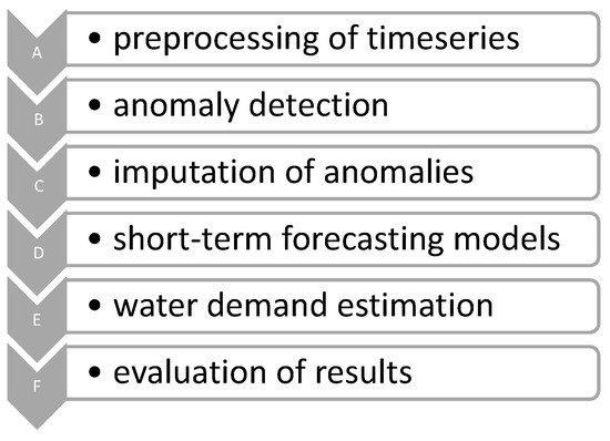
Figure 1.
Short-term time series forecasting methodology applied to water tank level data [16].
2.1. Study Area and Data Collection
The dataset used in this study consists of water level measurements from urban reservoirs in the Thessaloniki region (Greece). In previous work, the focus was on 21 central reservoirs in Eastern Thessaloniki, which were monitored over a 15-month period. For the present study, the dataset scope was expanded to 48 reservoirs, covering a broader area of approximately 300 km2 across metropolitan Thessaloniki.
Each reservoir’s water level was recorded using a SCADA (Supervisory Control and Data Acquisition) system, provided by EYATH S.A. at one-minute intervals, resulting in a high-resolution univariate time series of water levels. This high-frequency sampling over roughly two years generated an extensive dataset consisting of approximately 107 individual readings. The expanded dataset captures suburban water dynamics, including storage reservoirs and intermediary distribution facilities, reflecting a city-wide perspective on water demand patterns across residential, commercial, and industrial zones. By doubling the reservoir count and increasing geographic coverage, the dataset now represents a more comprehensive view of Thessaloniki’s full water network, which serves over one million inhabitants.
To ensure computational feasibility and align with operational forecasting needs, the raw data were aggregated to hourly intervals by averaging the 60 one-minute readings within each hour. This transformation preserves essential temporal trends while making large-scale analysis more tractable for modeling and forecasting applications.
The dataset also contains missing values and anomalies caused by sensor outages or telemetry errors. The proportion of missing timestamps per reservoir ranged from approximately 1.5% to 16% before data cleaning. Across the entire dataset, the overall missing value ratio was around 3%, meaning roughly 3 out of every 100 hourly entries were absent due to telemetry issues. Additionally, outliers accounted for approximately 1–2% of the recorded values, varying by reservoir.
The two-year span makes the forecasting task realistic and challenging. All raw data were stored in a Hadoop Distributed File System (HDFS) cluster for reliable and scalable access. Each large data file is broken into 128 MB blocks in HDFS, with replication (three copies per block by default) to ensure fault tolerance and high availability [18]. Although our experimental deployment uses a single physical node (described below), HDFS was configured to mimic a distributed environment, thereby facilitating seamless future scaling to multiple nodes.
2.2. HPC Infrastructure and Environment
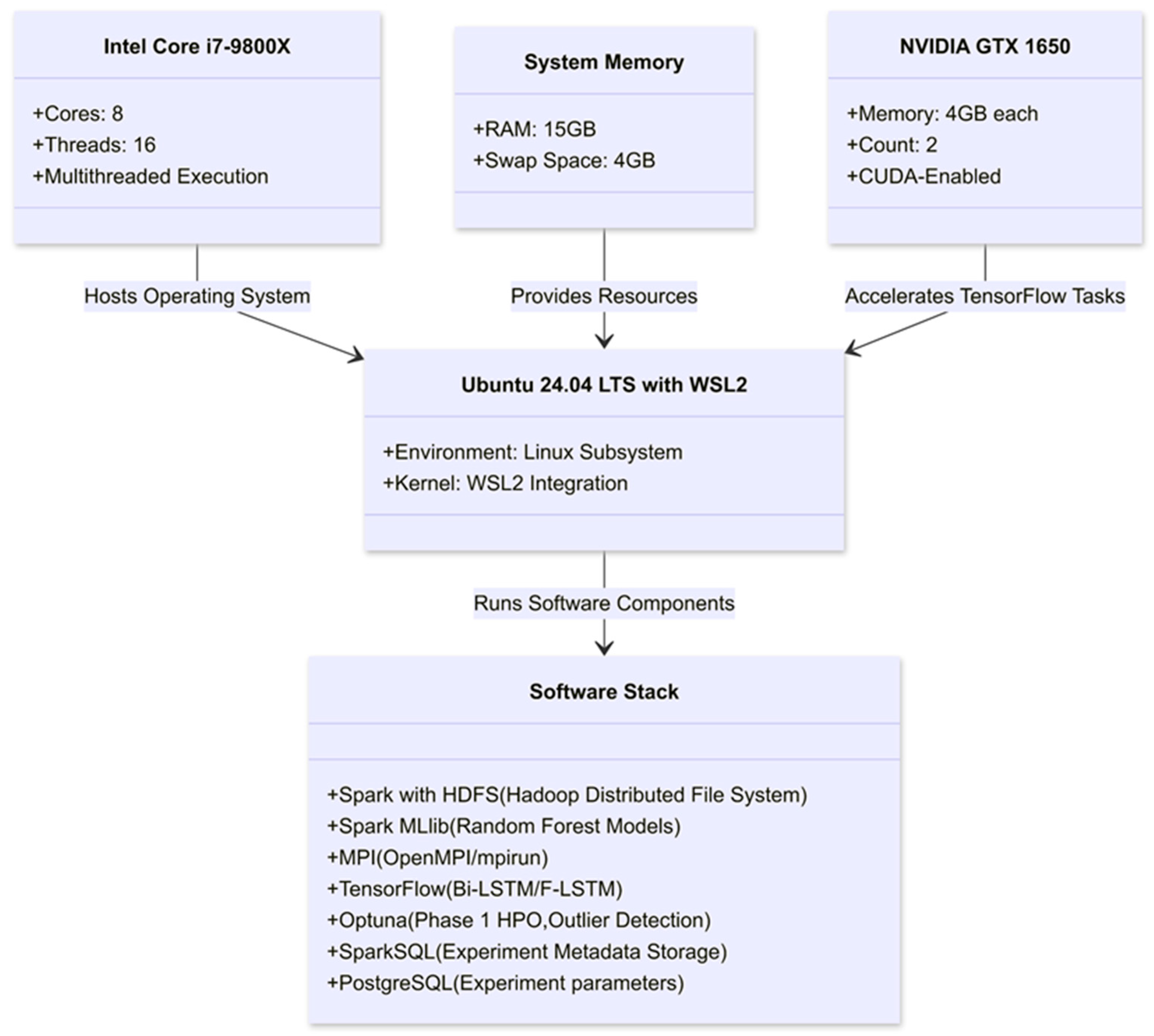
The computational environment as illustrated in Figure 2 was set up on a high-performance workstation running Ubuntu 24.04.1 LTS (via Windows Subsystem for Linux 2 on a Windows host). The hardware comprised an 8-core Intel Core i7-9800X CPU (16 threads), 15 GB of RAM, and two NVIDIA GeForce GTX 1650 GPUs (each with 4 GB VRAM). This modest-sized HPC setup was chosen to demonstrate that significant gains can be achieved even without a large cluster, and the pipeline is designed to scale out to multi-node clusters in future deployments. We leveraged Apache Hadoop (v3.3) for storage (HDFS, as noted) and Apache Spark (v3.3.2) for distributed data processing. Apache Spark was configured to use the local multi-core CPU resources as a cluster of executors, coordinating via a built-in Spark master. We also deployed OpenMPI (v4.1.1 via the mpirun interface) to launch parallel processes on the single node, effectively simulating an MPI cluster of ranks on the multi-core CPU. Deep learning tasks were implemented in Python (v3.9) using TensorFlow (v2.12 with Keras API), compiled with CUDA 12.6 to utilize the dual GPUs. The system’s software stack thus combined big-data processing tools (Spark, Hadoop), parallel computing libraries (MPI), and machine learning frameworks (TensorFlow, plus scikit-learn for some classical models). This integration was facilitated by the OS and driver configuration: running Spark and MPI inside WSL2 allowed direct access to Windows-installed GPU drivers for TensorFlow, ensuring that GPU acceleration functioned smoothly alongside the CPU-based distributed frameworks. Notably, TensorFlow was set to incrementally allocate GPU memory to avoid exhausting the 4 GB VRAM per card, and computations used mixed-precision where appropriate.
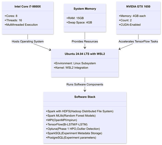
Figure 2.
Hardware Infrastructure and Software Stack.
As shown in Figure 3, a data processing pipeline was developed consisting of six scripts designed to support water demand forecasting using advanced machine learning techniques. The pipeline integrates several high-performance computing (HPC) and parallel processing technologies, including Apache Spark combined with the Hadoop Distributed File System (HDFS), the Message Passing Interface (MPI), and CUDA-enabled GPUs for accelerating TensorFlow computations. Additionally, Optuna was employed for hyperparameter optimization. The study further details the execution phases, optimization procedures, and logging mechanisms implemented throughout the forecasting process.
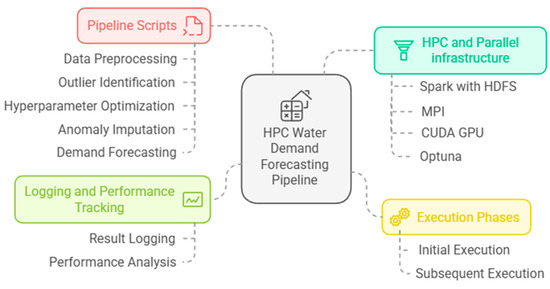
Figure 3.
HPC Water Demand Forecasting Pipeline.
2.3. Data Preprocessing Pipeline
The preparation of raw time series data for modeling involved several sequential steps executed within the pipeline. Each script corresponded to a specific stage in data cleaning or data impute, and the entire pipeline was orchestrated using the HPC and Parallel infrastructure.
2.3.1. Outlier Detection
Statistical techniques were applied to identify anomalies in the water level readings that could distort model training. Specifically, an Interquartile Range (IQR) filter and a moving standard deviation threshold were used to flag extreme deviations. These thresholds were not selected arbitrarily; instead, they were fine-tuned using the Optuna hyperparameter optimization tool to maximize anomaly detection performance [16].
By distributing the computation of these statistical metrics across MPI ranks, with each rank analyzing a subset of reservoirs, a significant speedup in outlier identification was achieved. Spark’s DataFrame APIs were utilized to efficiently read and slice the dataset for this step, taking advantage of in-memory distributed computation. Any detected outliers were either removed or capped based on domain-informed limits to prevent unrealistic values from biasing the models.
2.3.2. Data Cleaning and Imputation
Missing data is a common issue in sensor-based time-series datasets. To address gaps in the time series, a learned imputation approach was employed. For each reservoir’s time series, a pre-trained Bi-LSTM model was used to predict and fill missing values by leveraging temporal patterns from neighboring points.
The Bi-LSTM imputer, trained on historical data, captured both forward and backward temporal dependencies, ensuring plausible value reconstruction for missing entries. The imputation stage was parallelized, with multiple MPI ranks, each handling a subset of reservoir time series, loading a shared pre-trained model to generate imputations concurrently.
This parallelization enabled imputation across all 48 reservoirs simultaneously while leveraging GPU acceleration—each MPI rank offloaded its imputation task to a GPU via TensorFlow, significantly reducing processing time. As a result, even in cases where 5–10% of values were missing in some time segments, the pipeline was able to correct them within seconds. The effectiveness of LSTM-based imputation in preserving the integrity of subsequent forecasts is supported by prior research [16].
2.3.3. Normalization and Feature Engineering
After data cleaning, each reservoir’s time series was normalized using min-max scaling, which transformed water level values into a [0, 1] range—a prerequisite for ensuring stable training across machine learning algorithms. Normalization parameters (minimum and maximum values) were computed based on the training data split to prevent data leakage, and the same scaling was applied to the validation and test sets.
Additional features were engineered to enhance the predictive performance of the models, including hour of the day, day of the week and month indicators. These features allowed the models to account for known periodicities and consumption patterns.
To efficiently generate these features, Spark’s SQL and DataFrame operations were leveraged. Instead of iterating through reservoirs individually, feature extraction was vectorized and distributed, ensuring efficient processing across the dataset.
The dataset was then partitioned into training, validation, and testing sets, maintaining chronological order to replicate real-world forecasting conditions. This ensured that models were always trained on past data to predict future trends. The partitioning process was also managed using Spark, which allowed each executor to write out a portion of the final dataset in efficient Parquet format, minimizing I/O bottlenecks [19].
2.4. Parallel Model Training and HPC Integration
After preprocessing, the pipeline trains multiple forecasting models in parallel. The study retains the core models with the best performance from our prior study’s accuracy tests—bi-LSTM for imputation, f-LSTM for forecasting, and Random Forest Regressor (RFR) as a benchmark—optimized for the available hardware. The deep learning model, referred to as f-LSTM, is a univariate LSTM network optimized for forecasting next-day water demand based on recent historical data. The classical model is a Random Forest (RF) regression model, which serves as a baseline to assess the trade-offs between advanced deep learning techniques and traditional machine learning methods in HPC settings. All model training procedures were accelerated or distributed using HPC tools, as detailed below.
2.4.1. Apache Spark for Distributed Data Handling
Spark was used to manage the data feeding into model training and to parallelize the training of the Random Forest model. The RF training was implemented via Spark’s MLlib library, which can distribute tree-building across the cluster of executors. In our configuration, even though we run on a single machine, Spark creates one executor per CPU core, allowing the 100 decision trees (estimators) of the Random Forest to be built in parallel across threads. Spark’s Catalyst query optimizer automatically planned an efficient execution for reading the training data (stored in Parquet) and piping it into the MLlib routines [19] We also used Spark to parallelize the hyperparameter tuning for the Random Forest: multiple models with different random seeds were evaluated concurrently on different executors, and the best configuration (in terms of validation error) was selected. This demonstrates Spark’s strength in high-level parallelism without requiring explicit MPI-style code for certain tasks. Additionally, Spark oversaw the storage of intermediate results (like validation metrics) into a distributed SQL table (backed by Spark’s in-memory tables), which allowed for quick aggregation and analysis of results after training.
2.4.2. MPI for Parallel Algorithm Execution
While Spark handled data distribution and coarse-grained parallel tasks, MPI was employed for fine-grained parallel algorithms, especially related to deep learning models. One critical use of MPI in our pipeline was to parallelize hyperparameter optimization (HPO) for the bi-LSTM and f-LSTM models. We used Optuna for HPO, and by launching multiple Optuna trials across MPI ranks, we could explore the hyperparameter space (e.g., LSTM layer sizes, learning rates, dropout rates) much faster than serial search. Each MPI rank would run an independent training trial of the f-LSTM on a subset of data or with a unique hyperparameter set, and the results were gathered to decide the next set of trials. This MPI-based scatter-gather approach yielded near-linear speedups in the HPO phase, as each rank utilized both its CPU and (if available) GPU resources to train a model variant concurrently. MPI’s dynamic task allocation ensured that if one rank finished a trial early, it could request a new trial, thereby balancing the load and avoiding idle processors [10,11]. In practice, hardware memory limitations meant we ran a smaller number of parallel trials (e.g., five parallel trials at a time) to avoid GPU memory saturation, but the parallel approach still yielded a several-fold speedup in the hyperparameter search phase. Beyond HPO, MPI was also used to parallelize the training of multiple reservoir-specific models in experiments (for instance, training an LSTM for each reservoir simultaneously). In those cases, each rank was assigned a subset of reservoirs to train on, and the master process synchronized results, such as training time and error metrics.
2.4.3. GPU-Accelerated Deep Learning
The computationally most intensive tasks in the pipeline are the training of the Bi-LSTM and f-LSTM neural networks. We leveraged TensorFlow with CUDA to offload these operations to the GPUs. Both GPUs were utilized: we split the training load of a single model across the two GPUs using TensorFlow’s built-in multi-device strategy. We enabled mixed-precision training to reduce memory usage and increase throughput on the GPU, wherein less critical operations use 16-bit floating point precision and the rest use 32-bit [20]. This technique is known to accelerate training on GPUs while maintaining model accuracy, especially on hardware with limited memory. In our case, mixed precision allowed the 4 GB GPUs to handle relatively large batch sizes and sequence lengths without running out of memory, and it provided a modest speed boost due to the reduced data transfer and computation overhead on the GPU cores [20]. We also used TensorFlow’s GPU parallelism for batch processing: each training epoch processed batches of data in parallel on the GPU. The result is that model training times that would have been on the order of hours on CPU were brought down to minutes on GPU, enabling us to iterate quickly and even retrain models in near real-time as new data arrived.
2.4.4. Integration of Spark, MPI, and GPU
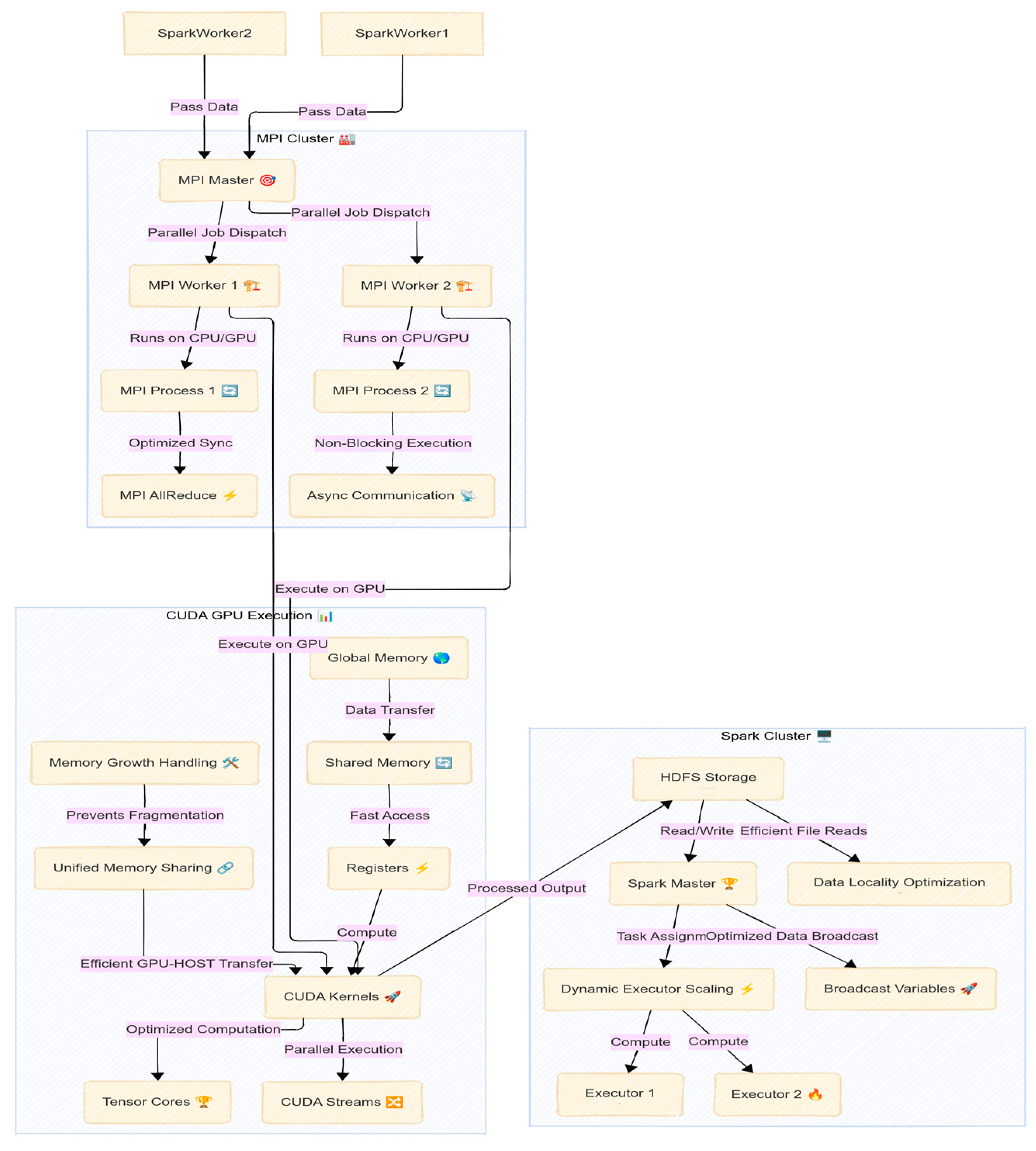
Figure 4 illustrates a key aspect of our methodology, which is the seamless integration of these frameworks. Spark handled the data loading and preprocessing, ensuring that when the training phase began, data was already partitioned and readily accessible in memory on the machine. Then, MPI took over to coordinate the parallel training tasks, and each MPI process invoked TensorFlow for the portions of training that could benefit from GPU acceleration. We carefully managed the interface between Spark and MPI: intermediate datasets (like the final feature matrix for training) were saved as distributed files (Parquet format) and then read by each MPI process locally. This approach avoided heavy data movement through the MPI communicator—each rank could directly read its portion of data from the local disk (thanks to HDFS’s replication on the single node, data locality was ensured [18]). Once training was completed, results (model parameters, metrics, logs) were gathered. Spark was then used again to aggregate these results, for example, merging the logs from each rank into a unified view and storing final models. By combining Spark’s ease of data handling with MPI’s control over parallel execution and GPUs’ raw computational power, the pipeline maximized resource utilization. This cohesive use of multiple HPC tools in one workflow is a distinguishing feature of our approach compared to previous efforts that might have used these tools in isolation.
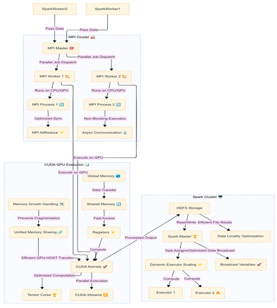
Figure 4.
Spark, MPi, and GPU Integration.
In developing the pipeline, we also implemented strategies for efficient resource use and fault tolerance. Data were stored and exchanged in columnar format (Parquet) to speed up I/O and allow selective loading of features, which reduced memory overhead [19]. We monitored memory usage throughout and used Python’s garbage collection triggers to preemptively clear buffers between pipeline stages, preventing memory bloat when handling large, in-memory datasets. For fault tolerance, we relied on Spark’s lineage-based recovery—if a data partition read failed or a node process died, Spark could recompute lost partitions automatically [21]. Similarly, for the MPI processes running long training jobs, we integrated periodic checkpointing: model weights and optimizer states were saved at intervals so that if a process or the program crashed, it could be resumed from the last checkpoint, following established MPI checkpointing practices [21]. These measures, while not the primary focus of this study, ensured that the pipeline was robust as well as fast. In summary, the methods above detail an HPC-driven approach that spans from data ingestion to model output, specifically tailored to improve both the scalability (ability to handle more data and more complex models) and efficiency (faster execution) of urban water demand forecasting tasks.
2.5. Data Availability
Restrictions apply to the availability of these data. Data were obtained from EYATH S.A. and are available from the authors with the permission of EYATH S.A. for scientific purposes.
2.6. Ethical Approval
This study did not involve human or animal subjects, and therefore, no specific ethical approval was required from an institutional review board for these aspects. The dataset utilized in this research consists exclusively of water level measurements from central reservoirs, expressed in water volume units, to forecast regional water demand. It is important to note that the data do not include any personal or sensitive information, such as residential water usage statistics or identifiable consumer data.
3. Results and Discussion
In this section, we present the experimental results of our HPC-enhanced water demand forecasting pipeline and discuss their implications. We evaluate both the forecasting accuracy of the models (Bi-LSTM + f-LSTM vs. the Random Forest baseline) and the computational performance of the system under different configurations. In particular, we compare a baseline serial execution against two HPC modes: (a) parallel training with all optimizations and (b) parallel inference, assuming models are pre-trained. We also address the rationale behind our modeling choices in light of the results and discuss the scalability and limitations of the approach.
3.1. Experimental Configurations and Performance Metrics
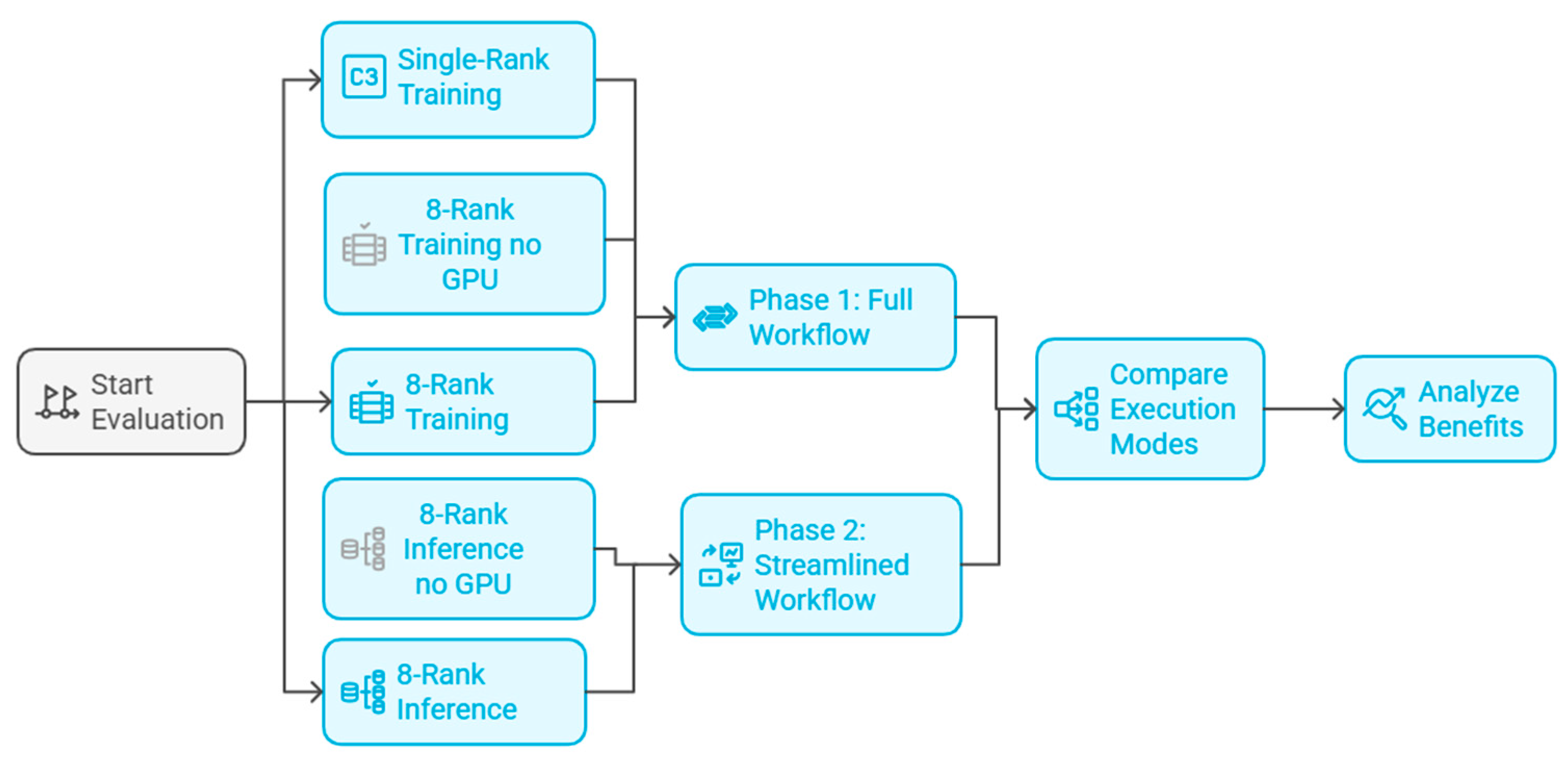
Figure 5 illustrates all experiments conducted on the single-node environment described in Section 2.2. We evaluated five pipeline configurations to assess the impact of parallelization, the use of pre-trained models and the use of GPUs:
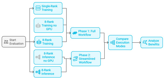
Figure 5.
Scalable HPC Pipeline for Water Demand Forecasting.
Baseline (Serial, 1 core): The entire pipeline runs essentially on a single CPU core, with no Spark, no MPI, and no GPU usage. All tasks are executed sequentially in a traditional manner. This represents how long the processing and forecasting would take without any HPC enhancements. It serves as a benchmark for speedup calculations.
Parallel Training (8 cores + GPUs): The full HPC pipeline is used, with 8 MPI processes utilizing all 8 CPU cores and both GPUs. In this scenario, models are trained from scratch on the training data and then used for forecasting. This simulates the situation of retraining models regularly (e.g., daily or weekly) before producing forecasts. It demonstrates the speedups due to parallel computing when models have to be trained for each cycle.
Parallel Training (8 cores, no GPUs): The full HPC pipeline is used, with 8 MPI processes utilizing all 8 CPU cores and no GPU usage. In this scenario, models are trained from scratch on the training data and then used for forecasting. This represents how long the processing and forecasting would take without any GPU accelerations.
Parallel Inference (8 cores + GPUs, Pre-trained): The pipeline is executed in parallel mode, but assuming that the models have already been trained (we skip the hyperparameter tuning and heavy retraining steps or use previously learned weights). Essentially, this configuration times the process of loading pre-trained models, updating them with the latest data if necessary, and generating forecasts. This scenario is relevant to operations where one might train models offline and then continuously deploy them for fast inference. It highlights how quickly forecasts can be produced when most learning has been done in advance.
Parallel Inference (8 cores, no GPUs, Pre-trained): The pipeline is executed in parallel mode, but assuming that the models have already been trained (we skip the hyperparameter tuning and heavy retraining steps or use previously learned weights) and the absence of GPU use. It serves as a benchmark for speedup calculations.
To quantify performance, we instrumented the pipeline to measure the execution time of each major stage under each configuration. We divided the pipeline into six stages for timing: (1) Data Preprocessing, (2) Outlier Detection, (3) Bi-LSTM Hyperparameter Optimization (HPO), (4) Bi-LSTM Imputation, (5) f-LSTM Forecasting, and (6) Random Forest Forecasting. These roughly correspond to the sequential steps in the pipeline. By measuring each stage, we can identify which parts benefit most from parallelism and which might still be bottlenecks. We also computed overall end-to-end runtimes for each configuration.
In addition to timing, we used standard metrics to evaluate forecasting accuracy: Root Mean Squared Error (RMSE) and Mean Absolute Error (MAE) between the predicted and actual water levels over a test period. We report errors in normalized units (since data were normalized), where an RMSE of 0.0 would indicate a perfect prediction, and, for context, the range of normalized data is [0, 1]. We primarily focus on RMSE as it penalizes larger errors more strongly, which is important for water management (large under- or over-estimations are especially undesirable). MAE is also examined for a direct average error magnitude. These accuracy metrics are averaged across all reservoirs in the test set.
For model training, we use a rolling-origin evaluation: we trained models on the first ~80% of the data and tested on the last ~20% (approximately the final 3 months) to evaluate how well the models forecasted from new data. In the parallel inference scenario, we simulated that the models had been pre-trained on the earlier data and only updated their state with the newest data points before forecasting.
By combining both accuracy and timing evaluations, we ensured that the HPC optimizations did not come at the cost of predictive performance, and we assessed the viability of the approach for operational use (where both accuracy and timeliness are crucial). The following subsections present the results for computational performance (timings and speedups) and then the forecasting accuracy and model comparisons.
3.2. Computational Performance: Serial vs. Parallel Pipeline
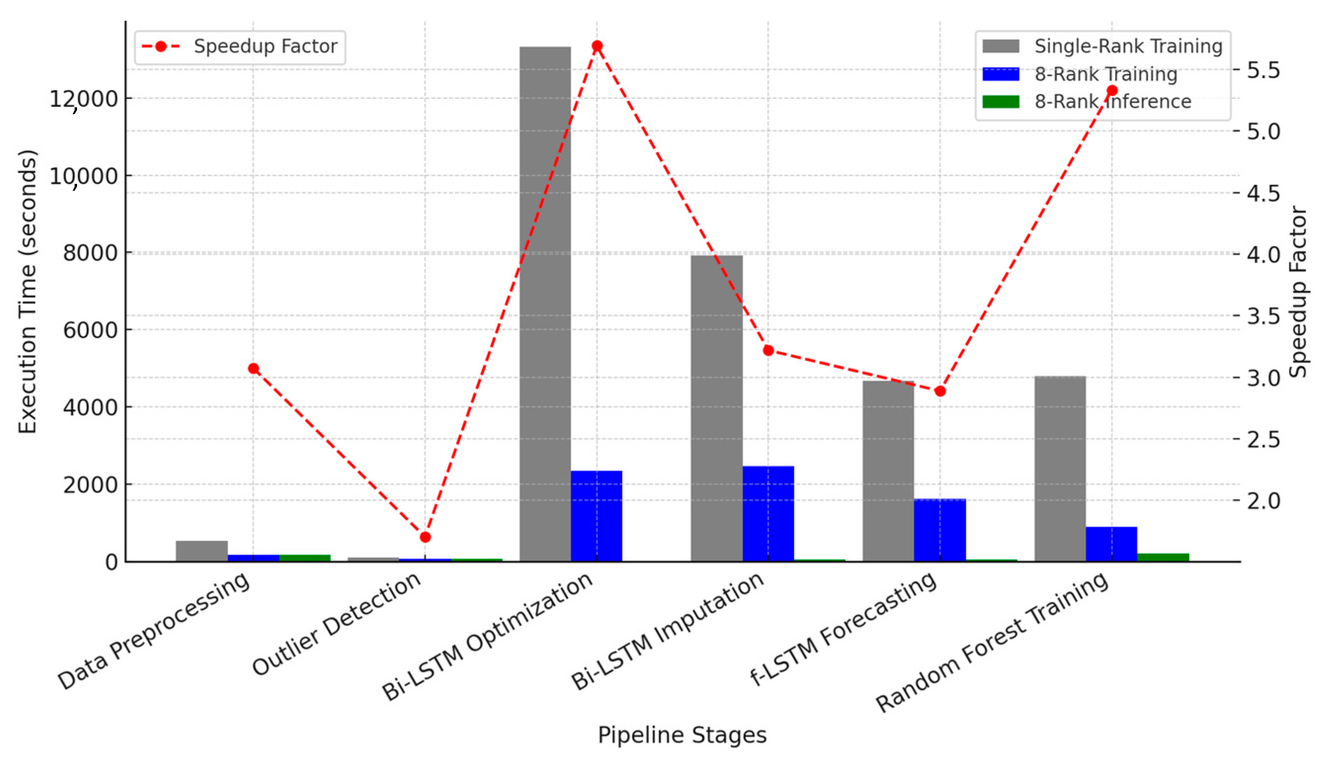
The execution times presented in Table 1 highlight the significant computational improvements achieved through high-performance computing (HPC) techniques. A comparison across Single-Rank Training (serial execution), 8-Rank Training (parallel execution with 8 MPI processes), and 8-Rank Inference (pre-trained models) demonstrates the impact of multi-core CPU processing, Spark-based data distribution, and GPU acceleration on various stages of the forecasting pipeline.

Table 1.
Average execution times per script under three configurations.
- Data Preprocessing
The Spark-based parallel implementation significantly reduced the data preprocessing time from 538 s (~9 min) in serial execution to 175 s (~3 min) in the 8-rank configuration, resulting in a 3× speedup. The speedup was limited by I/O operations (e.g., disk read/write) and Spark’s job scheduling overhead. However, the observed reduction indicates that distributed data processing significantly enhances computational efficiency. Further reductions in execution time could be achieved by increasing the number of processing cores or deploying a multi-node Spark cluster.
- Outlier Detection
Execution time for outlier detection was reduced from 104 s (serial) to 61 s (parallel execution, ~1.7× speedup). The smaller relative speedup can be attributed to Python-based computations under MPI, which do not scale as efficiently as Spark-based transformations. Despite the parallelization overhead, the reduction in execution time validates the effectiveness of distributed anomaly detection methods.
- Bi-LSTM Hyperparameter Optimization (HPO)
The hyperparameter tuning phase for the Bi-LSTM models exhibited substantial performance improvements. In serial execution, this stage required 13,320 s (~3.7 h), whereas parallel execution reduced it to 2340 s (~39 min), achieving a 5.7× speedup. The efficiency gain is attributed to MPI-distributed trials, which enable simultaneous evaluation of multiple hyperparameter configurations. In inference mode, hyperparameter tuning is skipped, leading to additional computational savings.
- Bi-LSTM Imputation
Training the Bi-LSTM imputation models for all reservoirs required 7920 s (~2.2 h) in the serial configuration, which was reduced to 2460 s (~41 min) under parallel execution, yielding a 3.2× speedup. The acceleration resulted from parallel execution across multiple MPI processes and GPU utilization, enabling concurrent model training.
In inference mode, execution time increased to 50 s as pre-trained models were loaded from the disk and applied to the dataset. The 50 s inference time accounts for TensorFlow session initialization, weight loading, and batch processing across all 48 reservoirs. Despite this overhead, the execution time remains acceptable for real-time forecasting applications.
- f-LSTM Forecasting
Training the forecasting LSTM (f-LSTM) models required 4680 s (~1.3 h) in serial execution, which was reduced to 1620 s (~27 min) in parallel execution, achieving a 2.9× speedup. The improvements are attributed to GPU acceleration, allowing multiple LSTM models to be trained concurrently.
During inference mode, execution time remained at 50 s, similar to Bi-LSTM inference, primarily due to model weight loading and sequential batch inference across reservoirs. Given that this step involves forecasting at an hourly resolution over a two-year horizon, 50 s represents a practical inference time for operational decision-making.
- Random Forest Forecasting (Spark MLlib)
The Random Forest (RF) training phase exhibited the highest computational cost in serial execution, requiring 4800 s (~80 min). The parallelized approach using Spark MLlib reduced training time to 900 s (~15 min), achieving a 5.3× speedup. This efficiency gain is attributed to Spark’s ability to distribute tree-building across multiple executors.
In inference mode, execution time dropped to 200 s (~3.3 min) as the pre-trained models were loaded instead of retrained. The significant reduction in computational cost demonstrates the efficacy of Spark’s distributed execution framework for ensemble learning models.
End-to-End Pipeline Performance
Figure 6 illustrates the execution time reductions achieved through HPC acceleration. The bar chart compares Single-Rank Training, 8-Rank Training, and 8-Rank Inference times for different pipeline stages. The red dashed line represents the speedup factors achieved by transitioning from serial to parallel execution.

Figure 6.
Execution Time Reduction via HPC Acceleration.
The total execution time across different configurations highlights the impact of HPC acceleration on the end-to-end pipeline. The serial execution mode (Single-Rank Training, using only one core) required approximately 523 min (~8 h and 43 min) to complete all tasks. This extensive runtime underscores the computational complexity of the forecasting pipeline when executed sequentially. In contrast, the 8-Rank Training mode, which utilizes eight CPU cores and two GPUs, significantly reduced the total execution time to 126 min (~2 h and 6 min). This represents an approximate 4.1× speedup, demonstrating the benefits of distributed computing and parallel execution.
Further improvements were observed in the 8-Rank Inference mode, where pre-trained models were used instead of retraining them from scratch. This configuration resulted in an execution time of approximately 9 min, making it suitable for real-time operational forecasting. The drastic reduction in inference time illustrates the efficiency of loading pre-trained models and executing forecasts on demand. By avoiding hyperparameter tuning and full model retraining, the inference pipeline achieves near-instantaneous execution, ensuring timely updates for water demand management systems.
The results demonstrate that parallel computing methods drastically reduce execution times, making real-time forecasting a feasible reality for large-scale urban water management. The inference pipeline, which completes itself in only 9 min, comfortably meets operational constraints where forecasting systems typically allow several hours for computation. Even with full retraining, the 126 min execution time is manageable within a daily or weekly retraining schedule, enabling the system to adapt to evolving water demand patterns.
These findings emphasize that leveraging Apache Spark, MPI, and GPU acceleration transforms the pipeline from an impractical 8 h computational burden into a scalable, near real-time forecasting solution. The key insight from this study is that the integration of distributed computing and deep learning optimization techniques ensures that large-scale water demand forecasting can be conducted efficiently, allowing for timely decision-making and resource allocation in urban water networks.
3.3. Computational Performance: GPU Acceleration vs CPU
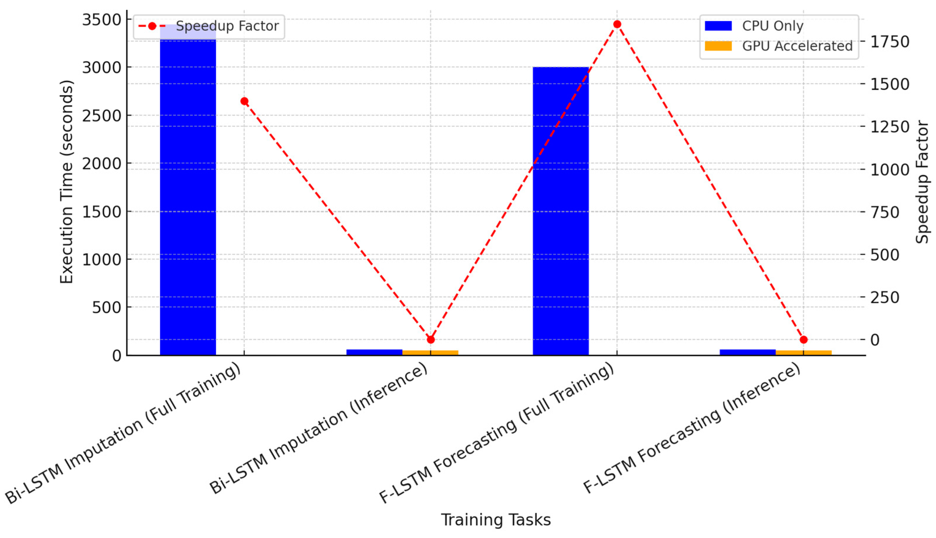
A core aim of this study is to quantify the performance gains from HPC enhancements. We measured the execution times of the key computational scripts with and without GPU support, focusing on the deep learning training tasks that are the most time-consuming.
Table 2 presents the execution times on a CPU-only environment (no GPU) for four major training tasks: (i) the pretraining of the forecasting LSTM (f-LSTM), (ii) the new (full) training of the forecasting LSTM, (iii) the pretraining of the imputation bi-LSTM, and (iv) the new/full training of the imputation bi-LSTM. These results were obtained on a modern 8-core CPU using a single thread for fairness in comparison (multi-threading was disabled for these particular measurements to represent a baseline).
Table 2.
Execution times of model training tasks on 8-Rank CPU with and without GPU accel3ration.
The results indicate significant execution time reductions when utilizing GPU acceleration, particularly in the full training phases of both the imputation Bi-LSTM and forecasting F-LSTM models.
Without GPU support, training the Bi-LSTM imputation model from scratch required 3444 s (~57 min) on the CPU, while training the forecasting LSTM model took 3000 s (~50 min). These durations confirm that deep learning training on the CPU alone introduces significant computational bottlenecks, which could hinder frequent model updates in an operational setting.
By leveraging GPU acceleration, the execution time for Bi-LSTM training was reduced to 2460 s (~41 min), achieving a 1.4× speedup. Similarly, the forecasting LSTM training time decreased from 3000 s to 1620 s (~27 min), resulting in a 1.85× improvement. Although not as drastic as the expected 10×–15× gains seen in other deep learning tasks, these results still demonstrate that GPU parallelism effectively reduces computational costs, making deep learning-based forecasting more efficient and practical.
The inference phase also exhibited moderate improvements with GPU acceleration. The Bi-LSTM inference time decreased from 60 s to 50 s, while the F-LSTM inference time improved from 58 s to 50 s. The relatively smaller improvements in inference time are expected, as inference tasks primarily involve forward passes, which are less computationally expensive than backpropagation-based training.
Figure 7 provides a visual comparison of execution times with and without GPU acceleration. The blue bars represent the CPU-only times, while the orange bars indicate GPU-accelerated execution. The difference in training times is clearly visible, with GPU-based execution significantly reducing training durations.
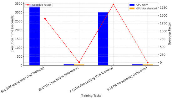
Figure 7.
Execution Time Comparison with and without GPU Acceleration.
The speedup factors for full model training were:
- 1.4× for Bi-LSTM training;
- 1.85× for F-LSTM training;
- 1.2× for Bi-LSTM inference;
- 1.16× for F-LSTM inference.
While the speedups for inferences are relatively small, the substantial reductions in training times demonstrate the value of GPU acceleration in enabling timely retraining of models for real-time applications.
These findings reinforce the importance of GPU parallelism in deep learning applications. GPUs excel at handling matrix-heavy operations in neural network training, particularly in backpropagation and gradient updates, making them essential for LSTM-based forecasting models.
From a practical deployment perspective, reducing training time from nearly an hour to approximately 27–41 min means that models can be retrained daily or multiple times per day, allowing the system to:
- Adapt to sudden changes in water consumption patterns;
- Update forecasts based on real-time sensor data;
- Perform continuous hyperparameter tuning to optimize performance.
Had GPUs not been used, training each model would have taken close to an hour, making frequent updates challenging. In contrast, GPU acceleration allows for efficient retraining, ensuring that the forecasting system remains accurate as new data is incorporated.
3.4. Model Performance and Accuracy
While the HPC enhancements significantly improve computational efficiency, the forecasting models must also achieve sufficient accuracy for the solution to be practical. To evaluate model performance, the forecasting LSTM (f-LSTM) and Random Forest Regression (RFR) models were tested on a held-out test dataset comprising the final months of data from each reservoir. Additionally, the imputation Bi-LSTM was evaluated on its ability to reconstruct missing data, with its accuracy compared against results from our prior study, as presented in Table 3.
Table 3.
Mean Accuracy Metrics Across Reservoirs.
The f-LSTM model achieved an average RMSE of 0.36 (in normalized units) and an MAE of 0.26 on the test set. The Random Forest achieved an average RMSE of 0.30 and MAE of 0.22. This means that, somewhat unexpectedly, the Random Forest slightly outperformed the LSTM in terms of accuracy on this particular test period—roughly a 17–20% lower RMSE. In real terms (denormalizing), these errors correspond to only a few centimeters of water level error given typical tank level ranges, which is quite acceptable for operational use. Both models thus provide a high level of accuracy, capturing the general demand patterns with only small deviations.
To investigate this result, we recall that our LSTM models did not undergo extensive hyperparameter tuning due to hardware limitations—only five trial configurations were attempted (Section 2.4.2). It is likely that the f-LSTM was not fully optimized and could be slightly under-fitting or over-fitting. The Random Forest, on the other hand, has fewer hyperparameters (number of trees, tree depth), which we tuned moderately, and it might inherently be more robust with the chosen features. In fact, in our previous study on a smaller dataset, an LSTM model did outperform Random Forest in most cases when properly tuned.
The Bi-LSTM imputation model was assessed by removing known data points and testing its ability to reconstruct them. The model achieved an RMSE of 0.38 (38% error), which is higher than the 7% error observed in prior studies. This deviation could be attributed to the larger dataset and increased variability in reservoir dynamics. However, despite the increased RMSE, the Bi-LSTM imputer ensured that the forecasting models received clean, gap-free input, minimizing disruptions from missing values.
Although the Random Forest model exhibited lower forecasting error, its adaptability in real-time settings is more limited compared to LSTM models. Once trained, a Random Forest model remains static, meaning that to integrate new data, full retraining is required. This could introduce latency and limit responsiveness to sudden changes in water demand patterns.
In contrast, LSTM models can be continuously updated with new data, making them more suitable for environments where real-time adaptation is critical. The HPC infrastructure developed in this study enables frequent retraining of LSTM models in just minutes, allowing them to adjust dynamically to new consumption trends without requiring full retraining cycles. This makes LSTM models a compelling choice for long-term deployment in urban water forecasting systems.
3.5. Parallel Pipeline Performance and Scalability
To validate the timing measurements, logs from the Spark History Server were examined, focusing on job durations, executor tasks, and shuffle overhead. The collected results, summarized in Table 4, highlight execution times, speedup, efficiency, throughput, memory usage, and I/O performance across different processing stages.
Table 4.
Time measurements and logs from Spark History Server.
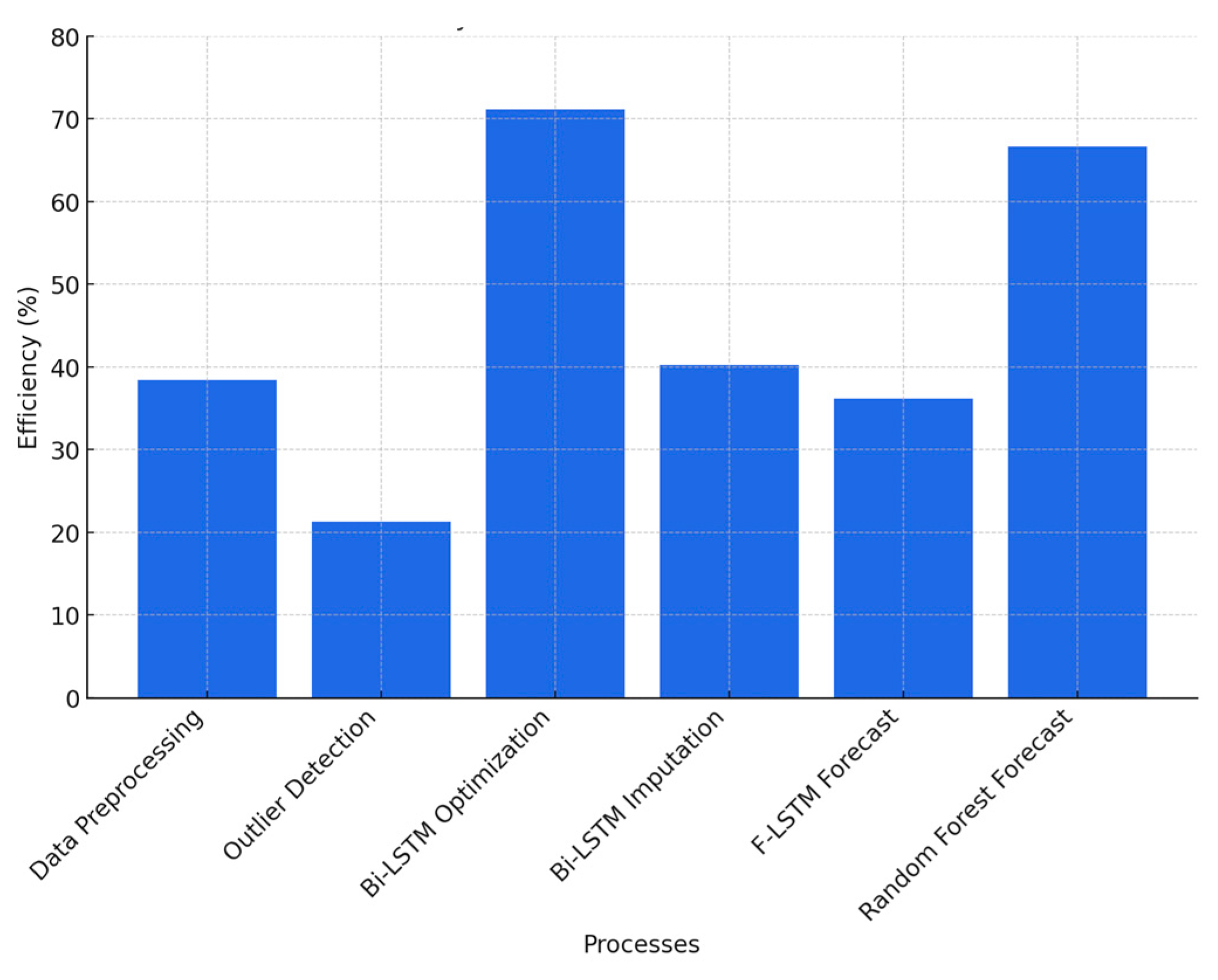
3.5.1. Efficiency of Parallel Execution
Parallel efficiency, defined as the ratio of speedup to the number of cores used, provides insight into how well computational resources are utilized. The Bi-LSTM Optimization step achieves 71.12% efficiency, suggesting that task parallelism is well-balanced with minimal communication overhead. In contrast, Outlier Detection exhibits the lowest efficiency at 21.25%, likely due to a lower computational load and increased synchronization costs among MPI ranks.
Figure 8 illustrates the efficiency trends across different processes, highlighting the computational phases where additional optimization may further enhance parallel performance.

Figure 8.
Efficiency trends across different processes.
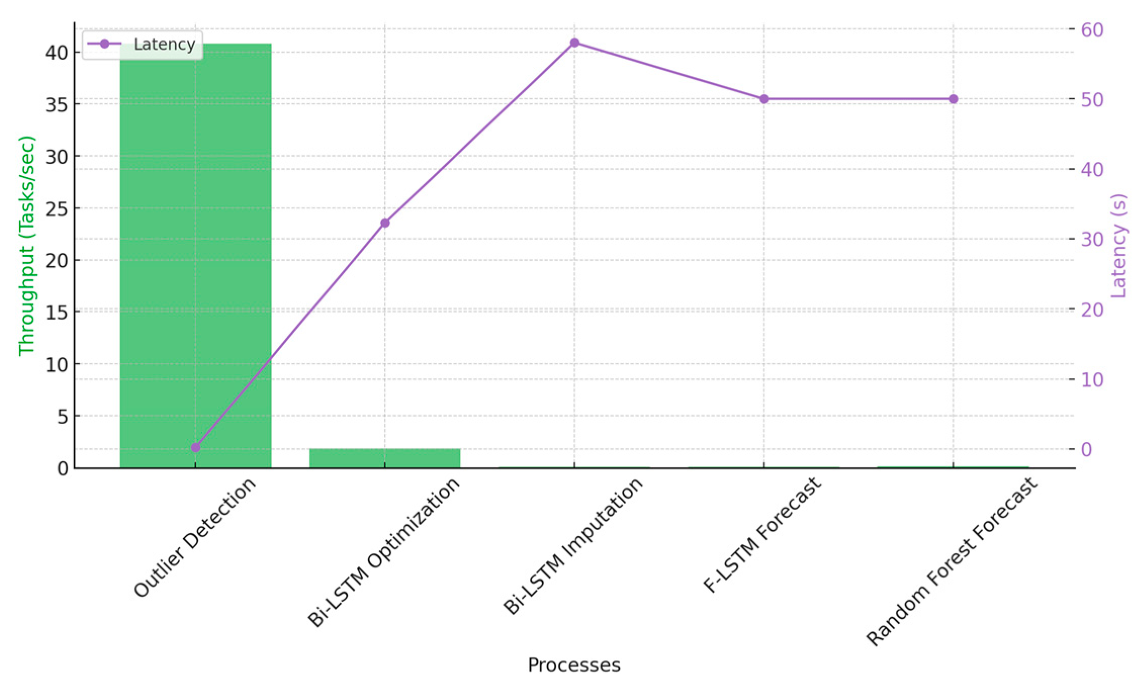
3.5.2. Throughput and Task Latency
Throughput, measured as the number of tasks completed per second, is an essential metric for evaluating the processing capability of parallel execution. The Outlier Detection stage achieves the highest throughput at 40.8 tasks per second, benefiting from its simple computations being easily parallelizable across cores. However, more complex stages such as Bi-LSTM Optimization and Imputation have lower throughput values of 1.86 and 0.078 tasks per second, respectively, due to their higher computational demands.
Interestingly, task latency remains nearly unchanged across different configurations, particularly in computationally expensive stages such as Bi-LSTM Optimization and Forecasting LSTM. While total execution time is significantly reduced through parallelization, the per-task execution duration remains largely consistent, indicating that the primary benefit of parallel computing in this context is increased task concurrency rather than per-task acceleration.
Figure 9 visualizes throughput performance across different computational stages.

Figure 9.
Throughput and Latency Across Processes.
3.5.3. Memory Utilization and Shuffle I/O
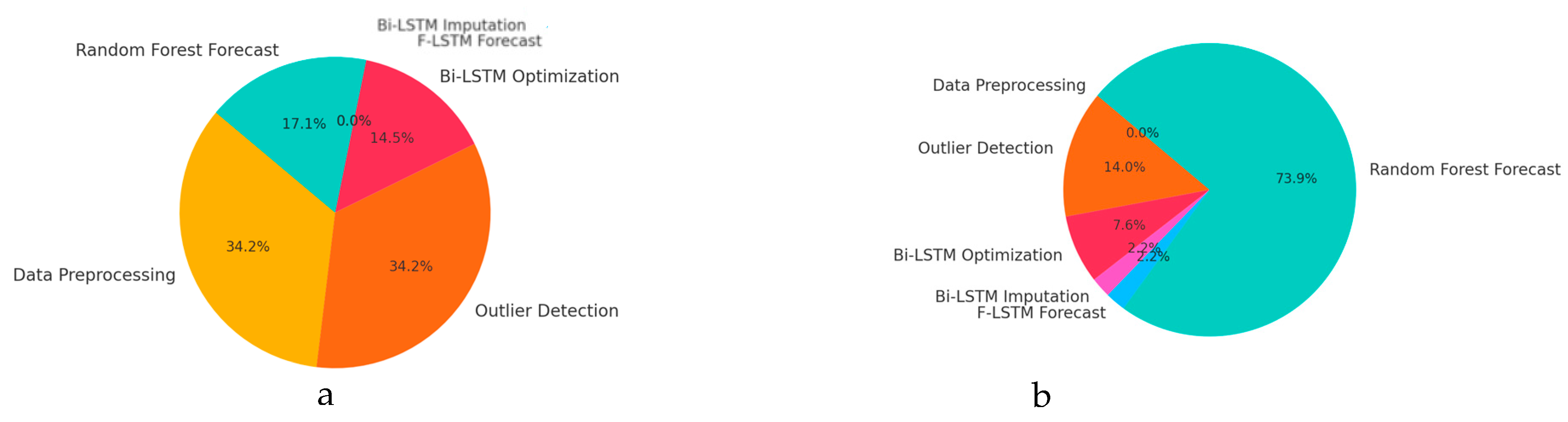
Memory management is a crucial factor in large-scale HPC applications. The Data Preprocessing and Outlier Detection steps consume the highest memory, with on-heap memory usage reaching 1024 MiB, while other tasks, such as Bi-LSTM Optimization and Forecasting LSTM, require significantly lower memory allocations. This suggests that data-intensive processes may require additional memory optimizations to enhance scalability further.
Shuffle I/O, representing the amount of data exchanged between distributed processes, varies significantly across computational stages. Random Forest Forecasting exhibits the highest shuffle I/O at 300 MiB, likely due to the need for extensive data exchange among Spark executors when constructing multiple decision trees. In contrast, LSTM-based processes show minimal shuffle activity (9.1 MiB), as neural network training is inherently less reliant on inter-process communication.
Figure 10a,b provide a comparative visualization of memory consumption and shuffle I/O across different processes.

Figure 10.
(a) Memory Utilization Distribution. (b) Shuffle I/O Distribution.
The strong scaling performance of the computational tasks demonstrates near-linear speedup with parallel execution. Notably, Bi-LSTM optimization and Random Forest forecasting achieve speedups exceeding 5× on an 8-core setup. This indicates that parallel processing effectively distributes computational loads, allowing tasks that would traditionally take hours on a single-core machine to be completed in significantly shorter timeframes. The ability to scale across multiple cores ensures that high-complexity computations can be executed efficiently, particularly in scenarios where large-scale data processing is required.
Deep learning workloads exhibit high efficiency in parallel execution, with the Bi-LSTM optimization stage achieving 71.12% efficiency. Similarly, LSTM-based forecasting tasks maintain efficiencies of approximately 40%, confirming that neural network training and inference scale effectively when distributed across multiple processing units. The ability to distribute neural network computations ensures that training deep learning models for real-time forecasting remains computationally feasible without excessive delays.
A key insight from the throughput and latency analysis is that throughput gains are achieved without significantly reducing task latency. The outlier detection stage demonstrates the highest throughput at 40.8 tasks per second, benefiting from parallel execution and the ability to process multiple data points simultaneously. However, deep learning-based tasks maintain lower throughput due to the higher computational demands of model training and inference. This suggests that while parallel execution accelerates processing speed, individual task completion times remain relatively stable.
Memory and shuffle I/O overheads vary across different processes, with Random Forest training requiring significantly higher memory (512 MiB) and shuffle I/O (300 MiB) compared to LSTM-based tasks. The higher memory consumption and disk I/O indicate that tree-based models impose a larger computational footprint due to their reliance on extensive data movement and decision tree construction. In contrast, deep learning-based tasks exhibit lower memory and I/O requirements, benefiting from optimized GPU acceleration.
The combination of parallel CPU execution, MPI task distribution, and GPU acceleration results in substantial computational gains. These improvements make real-time forecasting feasible while ensuring robust resource utilization across hardware components. By leveraging a hybrid HPC approach that incorporates multi-core processing and GPU acceleration, the computational efficiency of the forecasting pipeline is maximized, enabling faster execution times and more scalable forecasting capabilities.
3.6. Comparison with Related Studies
Our findings in computational performance can be put in perspective with other studies in the field of water demand forecasting and, more broadly, in time-series forecasting. Many prior works have concentrated on improving forecasting accuracy, often by developing novel model architectures or incorporating additional data. For example, Wang et al. (2023) [22] introduced the MACLA-LSTM architecture, which aimed to improve accuracy through a multi-component LSTM design. Their work demonstrated better predictive accuracy than baseline LSTMs, but the computational cost of their more complex architecture was not a focal point. In contrast, our study did not introduce a new model architecture but rather a data-centric approach that ensured that a strong existing model (standard LSTM) could be trained and executed efficiently at scale. The two approaches are complementary: one could potentially implement the MACLA-LSTM within our HPC framework to benefit from both improved accuracy and faster training.
Similarly, Zhou et al. (2022) [23] and Shan et al. (2023) [6] each proposed sophisticated hybrid models (CNN-LSTM and Attention-BiLSTM-XGBoost, respectively) to push forecast accuracy higher. These models involve more layers or components, which likely increases training time. While they report excellent accuracy, deploying such models in a real utility setting might face challenges if training or inference is slow. Our contribution to an HPC pipeline is highly relevant in such contexts: the parallel algorithms and GPU usage we demonstrated can be applied to those advanced models as well, reducing the barrier of computational feasibility. We respectfully note that those studies focused on algorithmic innovation, whereas we focus on engineering and scalability innovation; both are necessary for advancing the field. The present work essentially provides a template for how any advanced forecasting method can be operationalized in an efficient manner.
There are also studies that indirectly touch on computation through the lens of big data. For instance, Emami et al.’s (2022) [24] work in the agricultural water demand domain highlighted the use of big data and HPC for processing large datasets. Their emphasis was on leveraging remote sensing and multiple data sources, which inevitably requires robust computing infrastructure. Our work serves as a concrete case study of leveraging such infrastructure for the urban water sector. We go a step further in quantifying the performance gains, which is not commonly reported in typical forecasting papers. By presenting metrics like speedup and efficiency, we align with best practices in parallel computing research, bringing those into the water informatics arena.
Compared to general time-series forecasting literature, relatively few papers report on the runtime or scalability of their approaches. An exception is research in energy demand forecasting or smart grids, where sometimes the deployment aspects are discussed (e.g., needing to forecast in real-time on devices with limited resources). In water demand forecasting, the timeline is a bit more forgiving (forecasts are often daily or hourly, not every second), but as data volume grows (smart metering could provide much more granular data), the computational load will increase. Our results preemptively address this, showing that a pipeline can efficiently handle 48 streams of data and complex models in parallel.
In terms of limitations, we acknowledge that not all utilities have immediate access to high-end GPUs or HPC clusters. However, the landscape is changing—cloud computing services now offer on-demand HPC resources, and the cost of GPUs has been decreasing relative to the operational value they provide. Moreover, even in the absence of a GPU, our demonstration of multi-core CPU parallelism means that utilities with just a modern multi-core server can still achieve several-fold speedups by using parallel algorithms (e.g., using 8 cores, which is common in many servers or even high-end desktops).
Finally, it is worth comparing our HPC approach with alternative strategies like model simplification or approximation. One way to speed up computation is to use simpler models (e.g., smaller neural networks or linear models) or fewer data points (downsampling); while this can reduce runtime, it often comes at the cost of accuracy or detail. Our approach shows that we do not have to make that compromise—we kept the complex models and full dataset and instead used more computing power to manage them. This is in line with the trend in many fields where HPC enables the use of more sophisticated analyses that were previously too slow. For urban water management, this means utilities can harness state-of-the-art forecasting techniques without sacrificing the responsiveness of their decision-support systems.
In respectful contrast to others’ work, we emphasize that our scalability improvements do not diminish the contributions of previous studies on forecasting methodology; rather, we provide a means to deploy those contributions effectively.
3.7. Limitations and Areas for Improvement
Despite the demonstrated advantages of HPC and parallel computing in our water demand forecasting pipeline, certain limitations warrant attention:
Single-Node Setup: Our experiments used a single physical machine with limited GPU memory (4 GB per GTX 1650). A multi-node or more powerful multi-GPU setup would likely yield greater throughput but introduce added complexity.
Script-Based Workflow: Dividing the pipeline into six scripts, each reading and writing to HDFS, may introduce overhead. A more tightly coupled solution (e.g., end-to-end pipelines in Spark or direct GPU memory sharing) could reduce latency.
Hyperparameter Tuning Overhead: The Bi-LSTM Optimization step remains computationally heavy. Techniques like transfer learning, multi-fidelity optimization, or specialized hardware could mitigate this.
Addressing these issues could further enhance the pipeline’s suitability for real-world deployments, especially if real-time adaptation or multi-location scaling is required.
4. Conclusions
This study presents an integrated high-performance computing (HPC) pipeline that combines Apache Spark, Message Passing Interface (MPI), and GPU acceleration for efficient urban water demand forecasting. By leveraging parallel computing techniques, we demonstrate substantial computational improvements, reducing execution times by up to 5.7× for deep learning tasks and 5.3× for ensemble-based forecasting models. The results confirm that parallelized execution and GPU acceleration significantly enhance the scalability and efficiency of complex machine learning workflows in water management applications.
The computational analysis highlights key insights into parallel efficiency, throughput, and resource utilization. Bi-LSTM optimization achieved the highest efficiency (71.12%), demonstrating that deep learning workloads effectively leverage parallel execution. Meanwhile, Random Forest training required substantial memory (512 MiB) and shuffle I/O (300 MiB), indicating that tree-based models impose a larger computational footprint compared to LSTM-based approaches. The results further reveal that parallel computing primarily increases throughput without reducing per-task latency, reinforcing the need for optimized task scheduling and resource management in HPC environments.
From an operational perspective, the integration of Spark, MPI, and GPU-based deep learning enables near-real-time forecasting capabilities, ensuring timely decision-making in urban water resource management. The ability to reduce end-to-end pipeline execution from 8 h to just 9 min (inference with pre-trained models) demonstrates the feasibility of real-time deployment in large-scale infrastructure settings. Moreover, the robustness of the proposed system, validated through Spark History Server logs and MPI execution traces, ensures resilience to system failures and computational inefficiencies.
Compared to existing studies that emphasize forecasting accuracy, this study prioritizes scalability and computational efficiency. While prior research has introduced more complex forecasting architectures, their practical deployment is often constrained by computational costs. Our findings bridge this gap by demonstrating how existing models can be optimized for real-time execution using HPC frameworks without sacrificing predictive performance. The integration of Spark for distributed data preprocessing, MPI for parallel execution, and CUDA-enabled GPUs for deep learning ensures that state-of-the-art forecasting models can be operationalized effectively at scale.
Despite these advancements, certain limitations remain. The study was conducted on a single-node HPC setup, limiting scalability to eight CPU cores and two GPUs. Future work should explore multi-node deployments and cloud-based HPC solutions to assess the pipeline’s performance under distributed computing environments. Additionally, further optimization in hyperparameter tuning, possibly through transfer learning or multi-fidelity optimization, could reduce computational overhead while maintaining forecasting accuracy.
Overall, this research provides a scalable, efficient, and fault-tolerant forecasting solution for urban water management. The demonstrated computational gains validate the integration of parallel computing with deep learning techniques, making real-time forecasting feasible for large-scale water systems. Future research should focus on extending these methodologies to broader environmental applications, ensuring sustainable and data-driven resource management in complex urban infrastructures.
Author Contributions
Conceptualization, G.M. and A.T.; methodology, G.M. and A.T.; software, G.M.; validation, G.M. and A.T.; formal analysis, G.M.; investigation, G.M.; resources, G.M.; data curation, G.M.; writing—original draft preparation, G.M.; writing—review and editing, G.M., A.T. S.A. and V.G.V.; visualization, A.T. and V.G.V.; supervision, A.T., S.A. and V.G.V.; project administration, A.T., S.A. and V.G.V. All authors have read and agreed to the published version of the manuscript.
Funding
This research received no external funding.
Data Availability Statement
Restrictions apply to the availability of these data. Data were obtained from EYATH S.A. and are available from the authors with permission from EYATH S.A. Requests to access the datasets should be directed to gdpr-team@eyath.gr.
Acknowledgments
We acknowledge the support given by the International Hellenic University for providing the necessary resources and thank EYATH S.A. for their valuable assistance and provision of data.
Conflicts of Interest
The authors declare no conflicts of interest.
References
- Makridakis, S.; Spiliotis, E.; Assimakopoulos, V. Statistical and Machine Learning forecasting methods: Concerns and ways forward. PLoS ONE 2018, 13, e0194889. [Google Scholar] [CrossRef] [PubMed]
- Hochreiter, S.; Schmidhuber, J. Long Short-Term Memory. Neural Comput. 1997, 9, 1735–1780. [Google Scholar] [CrossRef] [PubMed]
- Graves, A. Generating Sequences With Recurrent Neural Networks. arXiv 2014, arXiv:1308.0850. [Google Scholar]
- Liu, Z.; Zhou, J.; Yang, X.; Zhao, Z.; Lv, Y. Research on Water Resource Modeling Based on Machine Learning Technologies. Water 2024, 16, 472. [Google Scholar] [CrossRef]
- Morales-Hernández, M.; Sharif, M.B.; Gangrade, S.; Dullo, T.T.; Kao, S.-C.; Kalyanapu, A.; Ghafoor, S.K.; Evans, K.J.; Madadi-Kandjani, E.; Hodges, B.R. High-performance computing in water resources hydrodynamics. J. Hydroinform. 2020, 22, 1217–1235. [Google Scholar] [CrossRef]
- Shan, S.; Ni, H.; Chen, G.; Lin, X.; Li, J. A Machine Learning Framework for Enhancing Short-Term Water Demand Forecasting Using Attention-BiLSTM Networks Integrated with XGBoost Residual Correction. Water 2023, 15, 3605. [Google Scholar] [CrossRef]
- Yang, C.; Meng, J.; Liu, B.; Wang, Z.; Wang, K. A Water Demand Forecasting Model Based on Generative Adversarial Networks and Multivariate Feature Fusion. Water 2024, 16, 1731. [Google Scholar] [CrossRef]
- Zaharia, M.; Chowdhury, M.; Franklin, M.; Shenker, S.; Stoica, I. Spark: Cluster Computing with Working Sets. In Proceedings of the 2nd USENIX Conference on Hot Topics in Cloud Computing, Boston, MA, USA, 22 June 2010; 10p. [Google Scholar]
- Dean, J.; Ghemawat, S. MapReduce: Simplified data processing on large clusters. Commun. ACM 2008, 51, 107–113. [Google Scholar] [CrossRef]
- Candelieri, A. Clustering and Support Vector Regression for Water Demand Forecasting and Anomaly Detection. Water 2017, 9, 224. [Google Scholar] [CrossRef]
- Delmas, V.; Soulaïmani, A. Multi-GPU implementation of a time-explicit finite volume solver for the Shallow-Water Equations using CUDA and a CUDA-Aware version of OpenMPI. arXiv 2020, arXiv:2010.14416. [Google Scholar]
- MPI4Spark: A Unified Analytics Framework for Big Data and HPC. Available online: https://par.nsf.gov/ (accessed on 3 March 2025).
- Altalhi, S.M.; Eassa, F.E.; Al-Ghamdi, A.S.-M.; Sharaf, S.A.; Alghamdi, A.M.; Almarhabi, K.A.; Khemakhem, M.A. An architecture for a tri-programming model-based parallel hybrid testing tool. Appl. Sci. 2023, 13, 11960. [Google Scholar] [CrossRef]
- Althiban, A.S.; Alharbi, H.M.; Al Khuzayem, L.A.; Eassa, F.E. Predicting software defects in hybrid MPI and OpenMP parallel programs using machine learning. Electronics 2024, 13, 182. [Google Scholar] [CrossRef]
- Elkabbany, G.F.; Ahmed, H.I.S.; Aslan, H.K.; Cho, Y.-I.; Abdallah, M.S. Lightweight computational complexity stepping up the NTRU post-quantum algorithm using parallel computing. Symmetry 2024, 16, 12. [Google Scholar] [CrossRef]
- Myllis, G.; Tsimpiris, A.; Vrana, V. Short-term water demand forecasting from univariate time series of water reservoir stations. Information 2024, 15, 605. [Google Scholar] [CrossRef]
- Ahmed, F.; Lin, J. Efficient imputation techniques for smart water systems. Water 2020, 12, 2481. [Google Scholar] [CrossRef]
- Shvachko, K.; Kuang, H.; Radia, S.; Chansler, R. The Hadoop distributed file system. In Proceedings of the 2010 IEEE 26th Symposium on Mass Storage Systems and Technologies (MSST), Incline Village, NV, USA, 3–7 May 2010. [Google Scholar] [CrossRef]
- Vohra, D. Apache Parquet. In Practical Hadoop Ecosystem; Apress: Berkeley, CA, USA, 2016; pp. 325–350. [Google Scholar] [CrossRef]
- Micikevicius, P.; Narang, S.; Alben, J.; Diamos, G.; Elsen, E.; Garcia, D.; Yao, J. Mixed precision training. arXiv 2018, arXiv:1710.03740. [Google Scholar]
- Armbrust, M.; Xin, R.S.; Lian, C.; Huai, Y.; Liu, D.; Bradley, J.; Zaharia, M. Spark SQL: Relational data processing in Spark. In Proceedings of the 2015 ACM SIGMOD International Conference on Management of Data, Melbourne, Australia, 31 May–4 June 2015; pp. 1383–1394. [Google Scholar] [CrossRef]
- Wang, K.; Ye, Z.; Wang, Z.; Liu, B.; Feng, T. MACLA-LSTM: A Novel Approach for Forecasting Water Demand. Sustainability 2023, 15, 3628. [Google Scholar] [CrossRef]
- Zhou, S.; Guo, S.; Du, B.; Huang, S.; Guo, J. A Hybrid Framework for Multivariate Time Series Forecasting of Daily Urban Water Demand Using Attention-Based Convolutional Neural Network and Long Short-Term Memory Network. Sustainability 2022, 14, 11086. [Google Scholar] [CrossRef]
- Emami, M.; Ahmadi, A.; Daccache, A.; Nazif, S.; Mousavi, S.-F.; Karami, H. County-Level Irrigation Water Demand Estimation Using Machine Learning: Case Study of California. Water 2022, 14, 1937. [Google Scholar] [CrossRef]


Disclaimer/Publisher’s Note: The statements, opinions and data contained in all publications are solely those of the individual author(s) and contributor(s) and not of MDPI and/or the editor(s). MDPI and/or the editor(s) disclaim responsibility for any injury to people or property resulting from any ideas, methods, instructions or products referred to in the content. |
© 2025 by the authors. Licensee MDPI, Basel, Switzerland. This article is an open access article distributed under the terms and conditions of the Creative Commons Attribution (CC BY) license (https://creativecommons.org/licenses/by/4.0/).