A Computationally Efficient Method for the Diagnosis of Defects in Rolling Bearings Based on Linear Predictive Coding

Abstract

Monitoring the condition of rolling bearings is a crucial task in many industries. An efficient tool for diagnosing bearing defects is necessary since they can lead to complete machine failure and significant economic losses. Traditional diagnosis solutions often rely on a complex artificial feature extraction process that is time-consuming, computationally expensive, and too complex to deploy in practice. In actual working conditions, however, the amount of labeled fault data available is relatively small, so a deep learning model with good generalization and high accuracy is difficult to train. This paper proposes a solution that uses a simple feedforward artificial neural network (NN) for classification and adopts the linear predictive coding (LPC) algorithm for feature extraction. The LPC algorithm finds several coefficients for a given signal segment containing information about the signal spectrum, which is sufficient for further classification. The LPC-NN solution was tested on the Case Western Reserve University (CWRU) and South Ural State University (SUSU) datasets. The results demonstrated that, in most cases, LPC-NN yielded an accuracy of 100%. The proposed method achieves higher diagnostic accuracy and stability to load changes than other advanced techniques, has a significantly improved time performance, and is conducive to real-time industrial fault diagnosis.

1. Introduction

Bearings are important components of many mechanical systems, including aircraft, vehicles, and CNC machines [1]. Due to the crucial role of these components, detecting and diagnosing any defects is an ongoing challenge [2] which has prompted researchers to look for solutions. The innovation of neural networks (NNs) has provided researchers with new solutions that primarily rely on deep learning [3,4,5].

In this case, fault diagnosis can be viewed as a pattern recognition problem where the pattern is related to the conditions of the bearings. The traditional method for defect classification can be divided into two main stages: a signal processing stage for identifying appropriate features, and a feature classification stage. The first stage, which involves feature extraction, depends on processing vibration-based signals either in the time domain, frequency domain, or sometimes in the time–frequency domain.

To understand the spectral formation of a signal, frequency-domain techniques are typically used. One of the most commonly used tools in this domain is the Fast Fourier Transform (FFT) [6]. Processing a signal in the time domain provides statistical features of the signal, such as zero crossing rate and signal frame power [7]. In most cases, operating conditions change over time, and the signal becomes non-stationary. Commonly used techniques in the time–frequency domain include the wavelet transform [8] and the Short-Time Fourier Transform (STFT) [9].

Recently, the Empirical Mode Decomposition (EMD) time–frequency signal analysis method has become widely used [10]. EMD can adaptively decompose a complex signal into several intrinsic mode function components, but it has the disadvantage of mode mixing when dealing with noisy non-stationary signals, which affects the efficiency of time–frequency analysis. To address this issue, the Ensemble EMD method was proposed [11], but it requires large computational resources [12]. Another method, Variational Mode Decomposition (VMD), uses adaptive Wiener filters, but the decomposition parameters of VMD significantly influence the decomposition results [13].

At the classification stage, machine learning algorithms are employed to use the resultant features from the processed signals as input and group them into clusters. In machine learning, there is a wide range of classifiers such as Support Vector Machines, Re-current Neural Networks (RNNs), and Convolution Neural Networks (CNNs) [14,15,16]. Jia [17] employed a deep normalized CNN for the imbalanced fault classification of machinery and analyzed its mechanism. Xu [18] introduced VMD and deep CNN to classify the faults of rolling bearings in wind turbines. Liu [19] proposed a fault diagnosis framework for rolling bearings using an RNN and Auto-Encoder.

The performance of these algorithms often has some limitations and high computational costs [20]. Deep learning-based methods have disadvantages mainly related to the need for a large number of labeled samples [21]. The performance of such methods is sensitive to an unbalanced dataset, where there is a larger amount of data collected related to healthy conditions. In addition, deep learning models are typically slow and require a significant amount of processing power and memory, making them very time- and re-source-intensive. In general, the trend in bearing failure diagnostics is towards more complex, deeper machine learning models. In actual working conditions, however, the amount of labeled fault data available is relatively small, so a deep learning model with good generalization and high accuracy is difficult to train. Some researchers are considering the need for alternative, simpler, and more application-oriented methods [22,23,24].

Linear predictive coding (LPC) is a speech coding algorithm [25] and is widely used in speech processing [26]. It approximates a signal sample at any moment as a linear combination of previous samples, and the weights for the linear combination are calculated by minimizing the mean squared error of the prediction for a signal frame. The resulting linear prediction coefficients are used to represent the frame. Although it has been traditionally used for speech, LPC is currently being improved and applied to non-speech signals as well [27,28].

In this paper, we apply LPC to vibration signals from rolling bearings. We evaluate our technique using the Case Western Reserve University (CWRU) [29] and South Ural State University (SUSU) [30] datasets. LPC is used to extract features from signals and then an NN is used to classify signals according to the extracted features. The advantages of this approach are the simplicity during the feature extraction stage, the small dimension of the resultant feature vector, and the simple architecture of the NN. This is particularly note-worthy in comparison with the increasingly sophisticated models used elsewhere for diagnosing bearing failures. Despite its simplicity, the proposed method achieves higher accuracy than some other advanced techniques.

The following are the main contributions of this article:

• A novel fault diagnosis method, which combines LPC and an NN, is proposed and used for bearing vibration signals.
• The LPC-NN method is less time-consuming and computationally less expensive compared to other advanced techniques.
• Experimental results on the CWRU and the SUSU datasets demonstrate that LPC-NN outperforms modern competitive techniques, achieving 100% accuracy in most cases.

The rest of the paper is organized as follows: The theoretical foundations of the LPC method, processing the signal for feature extraction, and the topology of the used NN are presented in Section 2. Section 3 describes the preparation of the dataset for the experiments. The experimental validation performed to evaluate the method is described in Section 4.

In Section 4.1 and Section 4.2, the performance of the LPC-NN method on one load and across different load domains was investigated. We used the CWRU dataset since the similar experiments were carried out on this dataset in [4,31]. The method LPC-NN turned out to be superior in accuracy to the powerful and computationally expensive method CNN-gcForest [4], and also the SVM, MLP, DNN, WDCNN, TICNN, and Ensemble TICNN [31] methods in some cases. In cases where LPC-NN did not give higher accuracy, it nevertheless demonstrated competitive performance. In Section 4.3, we compared the LPC-NN method in terms of time and accuracy with significantly different modern methods TSDIs-NN [32] and Hybrid CNN-MLP [33] for bearing fault diagnosis. For this, we used the SUSU dataset, on which the Hybrid CNN-MLP method was tested in [33], achieving superior accuracy and a significant improvement in time. Comparison with the TSDIs-NN method showed approximately the same computational costs, but a significant difference in accuracy in favor of the LPC-NN method. One of the traditional and widely used methods of bearing diagnostics is envelope analysis. However, in [33], we studied this method in detail in application to bearing fault diagnostics and showed that the traditional analysis of the envelope does not allow for accurate detection and localization of defects.

In recent years, data-driven fault diagnosis technology based on deep learning has attracted enormous attention. The LPC-NN method is in particular contrast to the increasingly complex models offered today for rolling bearing diagnostics and is conducive to real-time industrial fault diagnosis.

2. The Proposed LPC-NN Method

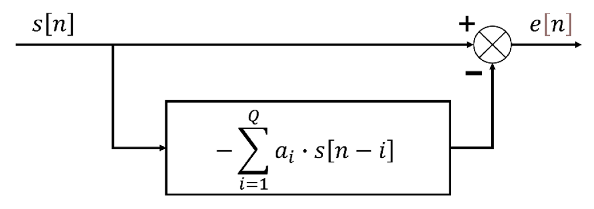
2.1. Linear Predictive Coding

The main use of the LPC algorithm is to encode speech signals at a low data rate. Figure 1 shows a block diagram of an LPC analysis system.

The key assumption is that the $n$th sample in the time series of a digital signal can be predicted by summing the $Q$ previous samples after multiplying each sample by a weight, following [34]:

$$\hat{s}\left[n\right]=-\sum _{i=1}^Q{a}_i·s\left[n-i\right].$$

(1)

Here, $s$ is the time series of the digital signal, $Q$ is the prediction order, and $a_i$ are the linear prediction coefficients. Thus, prediction of the sample at any moment is computed as a linear combination of the $Q$ previous samples of the signal, and hence, the prediction is linear. The LPC model is thus an autoregressive model [35].

The prediction error is equal to

$$e\left[n\right]=s\left[n\right]-\hat{s}\left[n\right].$$

(2)

The optimum predictor is the set of coefficients $a_i$, which produces a residual signal $e\left[n\right]$ with the least energy:

$$\rho =\sum _n{e}^2\left[n\right]=\sum _n{\left(s\left[n\right]+\sum _{i=1}^Q{a}_i·s\left[n-i\right]\right)}^2.$$

(3)

The linear prediction coefficients for the optimal case are computed by setting the partial derivatives of $\rho$ with respect to $a_i$ equal to zero, that is,

$${\displaystyle \frac{\partial \rho }{\partial a_k}}=2\sum _n\left(s\left[n\right]+\sum _{i=1}^Q{a}_i·s\left[n-i\right]\right)s\left[n-k\right]=0$$

(4)

for $k=\mathrm{1,2},\dots ,Q.$

Equation (4) can be rewritten as a system of $Q$ Yule–Walker linear equations involving autocorrelations:

$$\sum _{n}s\left[n\right]s\left[n-k\right]+\sum _{i=1}^Q{a}_i\sum _{n}s\left[n-i\right]s\left[n-k\right]=0$$

(5)

or

$$\sum _{i=1}^Q{a}_{i}R\left[i-k\right]=-R[k]$$

(6)

for $k=\mathrm{1,2},\dots ,Q,$ where $R\left[i-k\right]=\sum _{n}s\left[n-i\right]s\left[n-k\right],R\left[k\right]=\sum _{n}s\left[n\right]s\left[n-k\right]$. In matrix form, it can be written as a normal equation:

$$Ra=-r,$$

(7)

where

$$R=\left(\begin{array}{ccc}\begin{array}{cc}R\left[0\right]& R\left[1\right]\\ R\left[1\right]& R\left[0\right]\end{array}& \cdots & \begin{array}{c}R[Q-1]\\ R[Q-2]\end{array}\\ ⋮& \ddots & ⋮\\ \begin{array}{cc}R[Q-1]& R[Q-2]\end{array}& \dots & R\left[0\right]\end{array}\right)$$

(8)

and $a={\left[a_1 a_2 \dots a_Q \right]}^T$, $r={\left[R\left[1\right] R\left[2\right] \dots R\left[Q\right]\right]}^T$.

The matrix of the system (7) is a Toeplitz matrix, and linear prediction coefficients can be efficiently computed using the Levinson–Durbin recursion, starting with the first-order predictor and continuing recursively to find the coefficients of the $Q^{th}$-order predictor.

The system of Equation (7) can also be solved using Burg’s method [36]. The difference between the two algorithms is that Levinson’s method minimizes the forward prediction error while the Burg method minimizes the forward and backward prediction errors. Burg’s method is often superior to Levinson’s in accuracy (see, for example, [37]) but is more computationally expensive [38]. Since the main objective of this paper is to propose a computationally efficient method for bearing diagnostics, we use Levinson’s method implemented in the lpc function in Matlab.

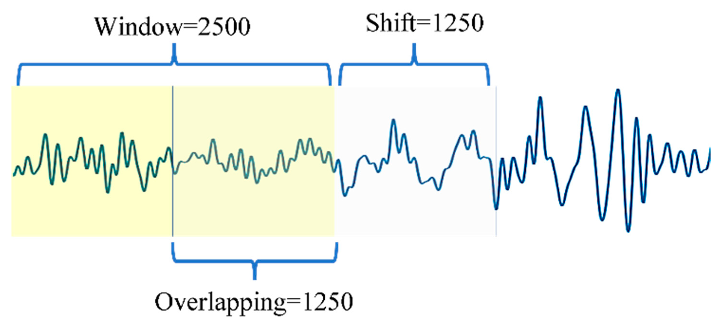
2.2. Feature Extraction

In order to understand the structure of the vibration signal from rolling bearing, we first examined their frequency components by applying FFT. Figure 2 shows some examples of spectrums for signals from the CWRU dataset that have different conditions. A detailed description of the CWRU dataset is provided in Section 3.1. Note here that these data were taken from an SK6205 bearing located at the drive end, and the acquisition frequency was 12 kHz. There are three fault types in the CWRU dataset (inner ring, outer ring, and ball) with three fault sizes. Figure 2 shows the spectra of the normal signal and signals with defects of the inner ring with different fault sizes and with a rotation speed of 1797 RPM.

It is clear that signals from different classes have different spectrums and fundamental components. It can also be observed that the spectrum of these signals resembles a speech-like spectrum; the number of spikes (formants) in the spectrum is not high and they are well spaced in each signal. Like a speech signal, the energy of a vibration signal is concentrated in narrow frequency bands. Linear prediction for speech signals models a mechanism that introduces correlation into the signal, the main source of which is the vocal tract [39]. For vibration signals, there is also a correlation caused by periodic impacts due to the presence of a defect. These properties suggest that LPC spectrum estimation works sufficiently well to track the formants of the signal, as is the case in speech processing.

The number of coefficients should correspond to the number of formants in the signal. Figure 3 shows the estimated spectrum of a healthy signal with zero loads on the bearing from the CWRU dataset using 12, 50, and 100 LPC coefficients. Using only 12 coefficients was not sufficient to obtain an accurate estimate, while using 100 coefficients did not significantly improve the estimate using 50 parameters. Therefore, using 50 parameters was suitable for achieving a smooth estimate.

Figure 4 shows the LPC spectrum for normal and defective signals from Figure 2a,b, with the number of LPC coefficients equal to 50. It can be seen that the compressed spectrum captures the main behavior in the original spectrum and, in addition, the spectra of signals of different types are significantly different.

As a method for choosing the number of LPC coefficients, we can also propose an analog of the “elbow” method, which is a common heuristic in mathematical optimization used to identify a point where diminishing returns are no longer worth the additional cost. Figure 5 shows the dependence of the mean squared error

$$MSE={\displaystyle \frac{1}{L}}\sum _{i=1}^L{\left({\left|X\right(f\left)\right|}_i-X_i^{est}\right)}^2$$

(9)

on the number of coefficients. Here, $\left|X\left(f\right)\right|-$ represents the power spectral density of a signal, and $X^{est}-$ denotes its estimate using a specific number of LPC coefficients. The idea is that after a certain number of coefficients, the spectrum estimate will already be quite good and further increases in the number of coefficients will not significantly improve it.

In Figure 5, for some signals of the CWRU dataset, we see a sharp elbow: a rapid decrease is replaced by a smoother one. Not all signals will exhibit such an elbow in the same location, so it is worth choosing the maximum number of coefficients.

Another way to select the model order is to use the criteria for autoregression models, the most famous of which are FPE, AIC, and MDL. These methods use a loss function which is minimized. The loss functions are as follows [40]:

$$FPE\left(p\right)={\displaystyle \frac{N+\left(p+1\right)}{N-\left(p+1\right)}}{\hat{\sigma }}^2,$$

(10)

$$AIC\left(p\right)=N\ln {\hat{\sigma }}^2+2p,$$

(11)

$$MDL\left(p\right)=N\ln {\hat{\sigma }}^2+p\ln N.$$

(12)

Here, $N$ is the number of samples, ${\hat{\sigma }}^2$ is the estimation of the variance in the residual, and $p$ is the order of the model. Note that sometimes other definitions can be found; for example, in the work [41], the loss function for $AIC\left(p\right)$ is determined by the formula

$$AIC\left(p\right)=\ln {\hat{\sigma }}^2+{\displaystyle \frac{2(p+1)}{N}}$$

(13)

and differs from Function (11) by a multiplier and a constant term. This is not of fundamental importance, since we are looking for the minimum point of the function.

We also applied these criteria to determining the model order. Figure 6 shows the corresponding dependencies on the number of model coefficients. These curves were plotted for a normal signal from the CWRU dataset. As can be seen, the curves for the FPE and AIC methods also resemble an elbow, and the MDL method demonstrates a clear minimum at an order value of approximately 50.

We will also use data from the SUSU dataset further (both datasets are described in detail below in Section 3). Figure 7 shows the dependences on the model order for a signal from a normal bearing from the SUSU dataset. It is clear that here, too, a model order of approximately 50 is also optimal. Therefore, throughout this article, we take this value of the model order.

We applied UMAP dimension reduction [42] to visualize the 50-dimensional LPC features in a 3D space for all signal types in the CWRU dataset with zero load. Different colors in Figure 8 represent different conditions. More information about these conditions can be found in Section 3.1. The results suggest that the features chosen are effective in classifying the fault types, as the points are not randomly located, but exhibit a certain order. The Normal class “0” is well separated from the other defective classes.

Figure 9 shows a similar arrangement of points in the SUSU dataset after dimensionality reduction using UMAP. This dataset contains five signal classes and is described in more detail in Section 3.2. Again, we observe that the data form distinct clusters corresponding to different types of signals.

We also used the t-SNE dimensionality reduction method [43], and similar results obtained with it are presented in Figure 10. It can be seen that this method, when reducing dimensionality, splits the data into clear, separated clusters: 10 for CWRU dataset and 5 for SUSU dataset. In general, the t-SNE method confirms the results obtained by UMAP and also indicates the informativeness of the LPC coefficients and the possibility of successfully solving the classification problem.

Figure 8, Figure 9 and Figure 10 demonstrate that the feature extracted by LPC are informative and relevant. It is worth noting the small dimension of the feature vector: each signal frame can be represented using only 50 parameters, which, as will be shown below, are enough for successful classification.

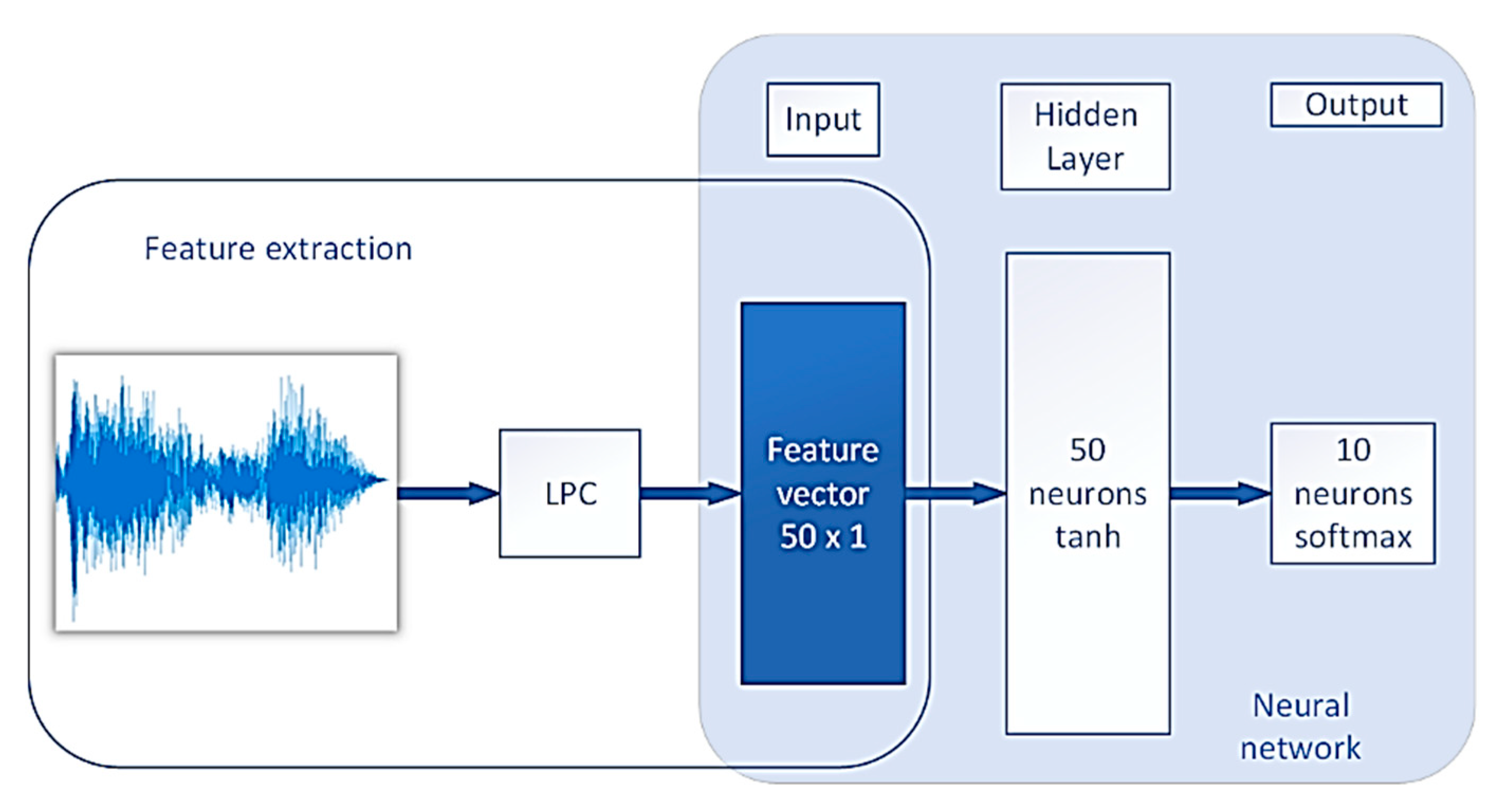
2.3. Proposed LPC-NN Method

In this section, we present the LPC-NN algorithm proposed in this paper for classifying vibration signals from bearings.

At the first stage, LPC coefficients are extracted from the signals using the LPC algorithm described in Section 2.1. These coefficients are features that are then fed to the input of the neural network. To increase the sample size of the training dataset, the signal is divided into short overlapping time frames (see Section 3.1). The set of 50 LPC coefficients calculated for each frame provides the training dataset for the classifying NN.

At the second stage, the 50 features are used as input for an NN with one hidden layer. Since the feature extraction process is simple, the NN has a simple structure. The input layer size is $50\times 1$, which is consistent with the dimension of the features extracted. This is followed by a layer of 50 neurons using the activation function “tanh”, and then a SoftMax layer calculates the probability of each of the possible outcomes. The number of neurons in the output layer is equal to the number of classes in the problem being considered. For the CWRU dataset, the output layer has 10 neurons, while for the SUSU dataset, it has 5 neurons.

Conventional NN techniques (categorical cross-entropy function, Adam optimizer, Keras EarlyStopping, and ModelCheckpoint callbacks) are applied [44]. When training the NN, we set aside 10% of the data for validation and monitor the accuracy on the validation set, and if there is no improvement within 50 epochs, training is stopped. Next, the model with the best accuracy on the validation set is selected. Figure 11 shows the full scheme of the method proposed.

For each dataset, feature extraction is used to generate 50 LPC coefficients, which are then supplied to the NN. This generates the probabilities that the original signal belongs to each of the 10 classes. In Section 4, we apply this algorithm to the CWRU and the SUSU datasets.

3. Description of Datasets

The proposed technique is evaluated using the CWRU and the SUSU datasets, which consist of real data obtained from experiments, rather than simulated data.

• The CWRU dataset was provided by Case Western Reserve University’s Bearing Data Center [45] and has been used extensively in rolling bearing fault diagnosis. CWRU vibration data were collected using accelerometers, which were attached to the housing of a mechanism. This is the traditional approach for collecting diagnostic information from such technological processes.
• The SUSU dataset [30] was provided by South Ural State University and obtained using a sensor mounted directly on the shaft. This method of mounting potentially provides increased sensitivity to defects.

Both datasets are described in more detail in Section 3.1 and Section 3.2.

For each time series, the first 70% of samples were used to create the training set, and the remaining 30% were used to create the corresponding test set, so that the training and testing time series did not overlap. The validation data were 10% of the test data.

3.1. The CWRU Dataset

From the entire dataset [45], a subset of time series with drive end fault characteristics was used; data were collected at a sampling frequency of 12 kHz. Four condition types were considered: normal (healthy), ball, outer, and inner faults. Each fault type can vary in severity; conveniently, all three fault types may be characterized by having a fault diameter, and the dataset contains examples for diameters of 0.007″, 0.014″, and 0.021″, so there are ten conditions in total. Each bearing was tested under four different loads: 0, 1, 2, and 3 HP. The motor speed varies according to the applied load: 1797, 1772, 1750, and 1730 RPM. For each recorded data sample, the motor speed is constant.

Table 1. Data classes in the CWRU dataset ¹.

Class Number	Fault Type	Diameter (Inches)
0 (no faults)	None	None
1	Ball	0.007
2	Ball	0.014
3	Ball	0.021
4	Inner	0.007
5	Inner	0.014
6	Inner	0.021
7	Outer	0.007
8	Outer	0.014
9	Outer	0.021

¹ Load is 0, 1, 2, and 3 HP for each class.

summarizes the cases. The cases under specific loads of 0, 1, 2, and 3 HP are called sub-datasets #1, 2, 3, and 4, respectively; the entire dataset contains all sub-datasets.

Typically, there is only about 20 s of data for each type of signal, which limits training, validating, and testing. Accordingly, the raw vibration signals were segmented into overlapping frames. Considering that the rotation speed was approximately equal to 1800 RPM, i.e., 30 revolutions per second, we took signal segments with a duration of about 1/5 of a second. During this time, we would have six shaft revolutions, during which the defect should manifest itself six times. Since the signal sampling frequency for the CWRU dataset is 12 kHz, it was convenient to take segments with a length of 2500 samples. Each frame contained 2500 samples, which is equivalent to $2500/\mathrm{12,000}=0.208$ s, with an overlapping percentage of 50 %, i.e., 1250 samples, as shown in Figure 12.

The number of frames obtained for each sub-dataset after the segmentation process is summarized in

Table 2. The number of frames for each sub-dataset in CWRU data.

Sub-Dataset	Number of Frames	Number of Training Frames	Number of Testing Frames
1	1066	747	319
2	1258	881	377
3	1258	881	377
4	1260	883	377
Entire dataset	4842	3392	1450

.

In the seminal work [45], each data record in the CWRU dataset was analyzed and classified into several categories based on their diagnostic interpretability, ranging from clearly diagnosable to non-diagnosable data. According to [45], ball faults were non-diagnosable using the three diagnostic methods described, highlighting the need for new approaches to achieve successful diagnoses for the datasets in this category.

3.2. The SUSU Dataset

This dataset was collected in the research laboratory of technical self-diagnostics and self-control of devices and systems at South Ural State University (Figure 13). A wireless acceleration sensor was used for data acquisition, which recorded two orthogonal linear accelerations and angular acceleration. The SUSU dataset contains signals for healthy bearings as well as bearings with inner race, ball, outer race, and combined defects. The specifications of the dataset are as follows:

• The motor rotation speed was constant at 1200 RPM.
• Data were obtained without load.
• The sampling frequency was 31175 Hz.
• The recorded signal length for each bearing condition was 64.1540 s.

Table 3. The number of frames for each sub-dataset in SUSU data.

Class Number	Fault Type	Number of Training Frames	Number of Testing Frames
0 (Normal)	None	2155	920
1	Ball	2155	920
2	Inner	2155	920
3	Outer	2155	920
4	Combined	2155	920

describes the signal classes and the number of frames in each class for the SUSU dataset. The signal segmentation technique used for the CWRU dataset was repeated with a frame length of 6494 samples, which is equivalent to 0.208 s.

Note that the number of training samples here is significantly larger than for CWRU (Table 2).

4. Experimental Results

This section contains the results of applying the proposed method to the CWRU and the SUSU datasets, along with a comparison to other known methods. Throughout this section, we use the LPC-NN method with the parameters’ values shown in

Table 4. Parameters values in experiments.

Parameter		Value
Number of trials Number of LPC coefficients Number of neurons in hidden layer Number of epochs Patience Length of signal frame, s		10
		50
		50
		500
		100
		0.208
Sampling rate, Hz	CWRU	12,000
	SUSU	31,175

. Given the stochastic nature of the proposed technique, all experiments were repeated 10 times, and the average results were recorded. Initially, the number of epochs was set to 500; however, due to the use of Keras callbacks—EarlyStopping and ModelCheckpoint—the number of training epochs was lower. These callbacks monitored the value of the loss function on the validation set and stopped the training process if it began to increase.

We used the value of the “patience” parameter equal to 100 epochs, meaning that we saved the model (with the smallest value of the loss function on the validation set). If there was no improvement in this value for 100 epochs, we stopped training and used the best previously saved model.

4.1. One-Load Experiment on CWRU Dataset

We repeated the experiment from [4], in which models were trained and tested on each specific dataset (from Table 2) using our new technique. The results are provided in

Table 5. Testing LPC-NN on all sub-datasets and on the entire dataset.

Sub-Dataset	Average Accuracy, %
1	100
2	99.71
3	100
4	100
Entire dataset	100

. The last outcome of the table corresponds to the case when the model was trained on the entire dataset, which consists of data with different load levels. This case is the most important in practice since this model is able to recognize the defect type for any load.

In most cases, the accuracy was 100%. Given the stochastic nature of the proposed technique, all experiments were repeated 10 times, and the average results are reported below. Misclassifications only occurred in the case of sub-dataset #2.

Figure 14 shows examples of classification results for two runs of sub-dataset #2 in the form of confusion matrices. The numbers in green on the diagonal correspond to the correct answers of the model, and the non-zero off-diagonal elements to its errors.

The ball defect class is the most challenging for the model trained on sub-dataset #2, and there may be confusion between objects of classes 1 (Ball 0.007″), 2 (Ball 0.014″), and 3 (Ball 0.021″) (Figure 14). In the subfigure on the left, the model predicts one sample of class 2 as a sample of class 1, in the subfigure on the right, the model assigns a sample of class 2 to class 3. Figure 14 shows the confusion matrices for only two program runs, but our detailed analysis indicates that confusion between the ball defect classes 1, 2, and 3 remains likely. This confirms the findings in [4] and [31] that the ball defect class is the most difficult to be accurately identified.

The paper [4] considered only vibration signals with loads of 1, 2, and 3 HP and used 900 samples (600 for training, 300 for testing). They also investigated the dataset as a whole.

Table 6. Comparing results of the proposed solution with solution in [4].

Sub-Dataset	CNN-gcForest [4], %	LPC-NN
2	98.24	99.73
3	99.51	100
4	99.79	100
Entire dataset	99.2	100

compares our results with those reported in [4].

The LPC-NN method is superior in accuracy to the very computationally complex method described in [4], which uses the continuous wavelet transform to convert bearing vibration data into images, and employs a convolutional NN to extract fault features, which are then scanned by gcForest and classified via a cascade forest strategy.

4.2. Performance Across Different Load Domains on CWRU Dataset

Another important test for the new approach is training the model on a specific sub-dataset and identifying the fault types belonging to another sub-dataset. For example, the model trained on a sub-dataset #1 (0 HP load) should be able to recognize the fault types under other loads. Obviously, after the load shifts, the diagnostic accuracies of any models decreased significantly.

Table 7. The results of training the LPC-NN method on one class and testing in other classes.

Class Label		Average Accuracy, %	Class Label		Average Accuracy, %
Training Sub-Dataset	Test Sub-Dataset		Training Sub-Dataset	Test Sub-Dataset
1	2	97.82	3	4	96.95
1	3	91.72	4	1	83.82
1	4	88.54	4	2	93.37
2	1	99.25	4	3	98.14
2	3	98.49	All	1	100
2	4	91.06	All	2	100
3	1	93.79	All	3	100
3	2	93.77	All	4	100

contains the results of training the LPC-NN method on one class only and predicting defects in other classes. The last four results in Table 7 correspond to the cases when the model trained on the entire dataset could perfectly predict classes for all sub-datasets. It can be seen that the accuracy of the method dropped significantly if the operating conditions of the bearing in the training and test datasets differed greatly.

A similar experiment was carried out by Zhang [31] although not all cases were considered. Note that the datasets A, B, and C in the paper [31] correspond to the sub-datasets #2, 3, and 4 in our paper.

Table 8. Comparing results of the proposed solution with solution in [31].

Training Sub-Dataset	Predicted Sub-Dataset	TICNN	Ensemble TICNN	LPC-NN
2	3	99.1	99.5	98.5
2	4	90.7	91.1	91
3	2	97.4	97.6	97.8
3	4	98.8	99.4	97
4	2	89.2	90.2	93.4
4	3	97.6	98.7	98.1
Average accuracy		95.5	96.1	96

summarizes the comparison between this work and the TICNN and Ensemble TICNN approaches in [31]. Note that the average accuracies for the methods SVM, MLP, DNN, and WDCNN are 66, 80, 78, and 90% [31], respectively, and lower than the average accuracy for LPC-NN.

The results in Table 8 show that the LPC-NN model is superior to Ensemble TICNN in the cases 3$\to 2$ and 4$\to 2$. In other cases, the LPC-NN model gives worse results, but even in these instances, the methods have comparable accuracy. Note that it is not mentioned in [31] how the data were divided into training and test sets. It remains unclear whether these two sets were non-intersecting, as in our case.

To study the influence of the number of LPC coefficients on the accuracy of the model, we also conducted the following experiment: We considered the number of LPC coefficients equal to 12, 50, and 100 and solved the problem of class prediction on the test sub-dataset 2 while training the model on sub-dataset 1. We thus considered three neural network models N-50-10 for N = 12, 50, 100.

Since the neural network training results are subject to stochastic changes, we trained each model 100 times and found the average accuracy of the model for each specific structure. The average accuracy value along with the time to train 100 models is given in

Table 9. Comparison of accuracy with different numbers of LPC coefficients at the NN input.

Number of LPC Coefficients	Time, s	Average Accuracy
12	2900	97.4
50	3200	98
100	2800	97.6

.

As can be seen, the best accuracy value is given by the 50-50-10 structure model with the number of LPC coefficients at the NN input equal to 50, which we found earlier based on the criteria for determining the model order. Note that this model, unlike the others, requires a little more time to train.

The training time for N = 12 is slightly less due to the smaller number of neural network parameters. The accuracy of this model 12-50-10 is lower, which is explained by the fact that the LPC model with N = 12 cannot capture all the informative features of the signals. The time for training the network with N = 100 is significantly less, which is explained by the larger capacity of the model 100-50-10 and the possible rapid overfitting of the network. This also explains the low accuracy of this model on the test dataset.

Thus, reducing the number of LPC coefficients is not advisable, since it leads to a decrease in the accuracy of the model and provides almost no improvement in time. Increasing the number of LPC coefficients requires a more powerful neural network. This will probably provide good accuracy but will require more training time.

4.3. Comparison of Computational Costs on SUSU Dataset

For each of the five classes in SUSU dataset, 70% of the available data were used for model training and validation; the remaining 30% were used for testing. A similar experiment on this dataset was carried out by Sinitsin et al. in [33], where they used the same dataset. However, ref. [33] used a hybrid model with mixed inputs. The linear acceleration signals were turned into time–frequency images using a Hilbert–Huang transform, which were the inputs for the CNN. The magnitude of the components of the frequency spectrum around the first and the second torsional natural frequencies of the shaft were summed to find the numbers N1 and N2 from the corresponding angular signals segments, which were inputs for the Multi-Layer Perceptron branch.

We compared the performance of our proposed LPC-NN method with the Hybrid CNN-MLP method [33] under the same conditions, and on the same data. For comparison, we also used different time-domain statistical indicators (TDSIs) as features for a neural network with two hidden layers of 30 and 20 neurons, respectively. We used six traditional TDSIs: peak, root mean square, crest factor, kurtosis, impulse factor, and shape factor. In addition to them, we used four new indicators, namely, TALAF and THIKAT [46], “kurtosis, crest factor and root mean square (KUCR)” [47], and INTHAR [48]. All experiments were repeated 10 times, and the average results are reported in

Table 10. Comparison of the average accuracy of the methods.

Method	Average Accuracy, %	Time for Feature Extraction for Each Frame, Seconds	Time for Model Training, Seconds
TDSIs-NN	76.8	0.038	25
Hybrid MLP-CNN	95.7	0.27	278
LPC-NN	98.3	0.00051	18

.

The LPC-NN method was more accurate, faster at extracting data, and quicker in model training. In [33], two components were used for feature extraction, which took over 500 times took longer than in the proposed method that uses a single acceleration component. Additionally, the training time for LPC-NN model was 15 times faster than for the hybrid model.

The TSDIs-NN and LPC-NN methods have approximately the same training time, but TSDIs-NN is much inferior in accuracy to LPC-NN. For a detailed comparison between the methods, see

Table 11. $f_1$-score comparison.

	TDSIs-NN	Hybrid CNN-MLP	LPC-NN
Normal	0.70	1.00	1.00
Inner	0.86	0.96	0.96
Outer	0.78	0.96	1.00
Ball	0.70	0.92	1.00
Comb	0.84	0.95	0.96
Accuracy	0.78	0.96	0.98

, which shows the accuracy and $f_1$-score values of all approaches obtained in the last run out of 10. In this run, TSDIs-NN and Hybrid CNN-MLP model achieved 78% and 96% accuracy, while LPC-NN achieved 98% accuracy.

The $f_1$-score assesses the classification model’s performance and is calculated based on precision and recall:

$$f_1={\displaystyle \frac{2·precision·recall}{precision+recall}}.$$

(14)

Precision is defined as the number of true positive results divided by the number of all positive results, including those that were not identified correctly. Recall, on the other hand, is the number of true positive results divided by the total number of all samples that should have been identified as positive. The best value of $f_1$-score is 1 and the worst is 0.

The Normal class achieved the best f1-score value for Hybrid CNN-MLP and LPC-NN models. However, this class is difficult for the TDSIs-NN model and, in general, its $f_1$-score values are worse for all classes.

Note that all the results presented in Section 4 are available as Jupiter Notebooks [30] in the LPC-NN folder. All experiments were implemented on a computer with Intel i7-8550 K 1.80 GHz CPU, 12.0 GB RAM.

5. Discussion

This study developed a novel approach for rolling bearing diagnosis, which relies on the spectrum estimation of the signal, using an LPC algorithm. The LPC coefficients are used as input vectors for a simple NN that can predict the fault type with high precision. The benefits of the proposed LPC-NN approach are as follows: (1) it is easy to implement, (2) the feature vector size is small, containing only 50 values, and (3) the NN used is simple, containing only one hidden layer. The performance of LPC-NN was verified under different operating conditions and on two experimental datasets CWRU and SUSU.

In our experimental studies, the LPC-NN method outperformed the powerful method CNN-gcForest for single-load CWRU data. The LPC-NN method demonstrated good robustness under changing operating conditions, surpassing the robustness of methods such as SVM, MLP, DNN, and WDCNN. Although the proposed method LPC-NN was sometimes inferior in accuracy to the extremely powerful method Ensemble TICNN, it showed comparable results. Given approximately the same accuracy values, the relative simplicity of the LPC-NN method should be noted.

The LPC-NN method also outperformed the Hybrid MLP-CNN method in terms of accuracy and computational costs when tested on the SUSU dataset. Compared to the TDSIs-NN method with a similar running time, LPC-NN demonstrated significantly greater accuracy.

Further research will focus on determining whether the features extracted using the LPC algorithm can also serve as input for another classifier (such as SVM and Logistic Regression) and on testing the method’s performance under conditions of data imbalance and high noise.

The methods being developed for diagnosing rotating equipment are becoming more reliable, efficient, accurate, and superior over time, often combined with artificial intelligence algorithms. However, they are also becoming increasingly computationally expensive and deep, requiring a large set of labeled data for training. In reality, such methods are unlikely to be implemented in industrial enterprises; therefore, effective methods suitable for practical applications are needed. The development of these methods will be the focus of many scientific researchers in the future.

References

1. Peng, B.; Bi, Y.; Xue, B.; Zhang, M.; Wan, S. A Survey on Fault Diagnosis of Rolling Bearings. Algorithms 2022, 15, 347. [Google Scholar] [CrossRef]
2. Liu, F.; Gao, S.; Tian, Z.; Liu, D. A new time-frequency analysis method based on single mode function decomposition for offshore wind turbines. Mar. Struct. 2020, 72, 102782. [Google Scholar] [CrossRef]
3. Qi, R.; Zhang, J.; Spencer, K. A Review on Data-Driven Condition Monitoring of Industrial Equipment. Algorithms 2023, 16, 9. [Google Scholar] [CrossRef]
4. Xu, Y.; Li, Z.; Wang, S.; Li, W.; Sarkodie-Gyan, T.; Feng, S. A hybrid deep-learning model for fault diagnosis of rolling bearings. Measurement 2021, 169, 108502. [Google Scholar] [CrossRef]
5. Han, H.; Wang, H.; Liu, Z.; Wang, J. Intelligent vibration signal denoising method based on non-local fully convolutional neural network for rolling bearings. ISA Trans. 2022, 122, 13–23. [Google Scholar] [CrossRef] [PubMed]
6. Wang, W.; Ismail, F. An enhanced bispectrum technique with auxiliary frequency injection for induction motor health condition monitoring. IEEE Trans. Instrum. Meas. 2015, 64, 2679–2687. [Google Scholar] [CrossRef]
7. Zhen, L.; Zhengjia, H.; Yanyang, Z.; Xuefeng, C. Bearing condition monitoring based on shock pulse method and improved redundant lifting scheme. Math. Comput. Simul. 2008, 79, 318–338. [Google Scholar] [CrossRef]
8. Luo, G.Y.; Osypiw, D.; Irle, M. On-line vibration analysis with fast continuous wavelet algorithm for condition monitoring of bearing. J. Vib. Control 2003, 9, 931–947. [Google Scholar] [CrossRef]
9. Wang, W.J.; McFadden, P.D. Early detection of gear failure by vibration analysis and calculation of the time-frequency distribution. Mech. Syst. Signal Process. 1993, 7, 193–203. [Google Scholar] [CrossRef]
10. Huang, N.E.; Shen, Z.; Long, S.R.; Wu, M.C.; Snin, H.H.; Zheng, Q.; Yen, N.C.; Tung, C.C.; Liu, H.H. The empirical mode decomposition and the Hilbert spectrum for nonlinear and non-stationary time series analysis. Proc. R. Soc. Lond. A 1998, 454, 903–995. [Google Scholar] [CrossRef]
11. Huang, N.E.; Wu, Z. A review on Hilbert-Huang transform: Method and its applications to geophysical studies. Rev. Geophys. 2008, 46, RG2006. [Google Scholar] [CrossRef]
12. Parey, A.; Badaoui, M.; Guillet, F.; Tandon, N. Dynamic modelling of spur gear pair and application of empirical mode decomposition-based statistical analysis for early detection of localized tooth defect. J. Sound Vib. 2006, 294, 547–561. [Google Scholar] [CrossRef]
13. Jiang, X.; Wang, J.; Shi, J.; Shen, C.; Huang, W.; Zhu, Z. A coarse-to-fine decomposing strategy of VMD for extraction of weak repetitive transients in fault diagnosis of rotating machines. Mech. Syst. Signal Process. 2019, 116, 668–692. [Google Scholar] [CrossRef]
14. Yuan, Z.; Zhang, L.; Duan, L.; Li, T. Intelligent Fault Diagnosis of Rolling Element Bearings Based on HHT and CNN. In Proceedings of the 2018 Prognostics and System Health Management Conference (PHM-Chongqing), Chongqing, China, 26–28 October 2018; pp. 292–296. [Google Scholar] [CrossRef]
15. Zou, Y.; Zhang, X.; Zhao, W.; Liu, T. Rolling Bearing Fault Diagnosis Based on Optimized VMD Combining Signal Features and Improved CNN. World Electr. Veh. J. 2024, 15, 544. [Google Scholar] [CrossRef]
16. Shao, H.; Jiang, H.; Zhao, H.; Wang, F. A novel deep autoencoder feature learning method for rotating machinery fault diagnosis. Mech. Syst. Signal Process. 2017, 95, 187–204. [Google Scholar] [CrossRef]
17. Jia, F.; Lei, Y.; Lu, N.; Xing, S. Deep normalized convolutional neural network for imbalanced fault classification of machinery and its understanding via visualization. Mech. Syst. Signal Process. 2018, 110, 349–367. [Google Scholar] [CrossRef]
18. Xu, Z.; Li, C.; Yang, Y. Fault diagnosis of rolling bearing of wind turbines based on the Variational Mode Decomposition and Deep Convolutional Neural Networks. Appl. Soft Comput. 2020, 95, 106515. [Google Scholar] [CrossRef]
19. Liu, H.; Zhou, J.; Zheng, Y.; Jiang, W.; Zhang, Y. Fault diagnosis of rolling bearings with recurrent neural network-based autoencoders. ISA Trans. 2018, 77, 167–178. [Google Scholar] [CrossRef]
20. Saufi, S.R.; bin Ahmad, Z.A.; Leong, M.S.; Lim, M.H. Challenges and opportunities of deep learning models for machinery fault detection and diagnosis: A review. IEEE Access 2019, 7, 122644–122662. [Google Scholar] [CrossRef]
21. Sun, T.; Gao, J. New Fault Diagnosis Method for Rolling Bearings Based on Improved Residual Shrinkage Network Combined with Transfer Learning. Sensors 2024, 24, 5700. [Google Scholar] [CrossRef]
22. Chen, Z.; Cen, J.; Xiong, J. Rolling Bearing Fault Diagnosis Using Time-Frequency Analysis and Deep Transfer Convolutional Neural Network. IEEE Access 2020, 8, 150248–150261. [Google Scholar] [CrossRef]
23. Zhang, W.; Peng, G.; Li, C.; Chen, Y.; Zhang, Z. A New Deep Learning Model for Fault Diagnosis with Good Anti-Noise and Domain Adaptation Ability on Raw Vibration Signals. Sensors 2017, 17, 425. [Google Scholar] [CrossRef] [PubMed]
24. Fang, H.; Deng, J.; Zhao, B.; Shi, Y.; Zhou, J.; Shao, S. LEFE-Net: A Lightweight Efficient Feature Extraction Network with Strong Robustness for Bearing Fault Diagnosis. IEEE Trans. Instrum. Meas. 2021, 70, 3513311. [Google Scholar] [CrossRef]
25. Chu, W.C. Speech Coding Algorithms: Foundation and Evolution of Standardized Coders; John Wiley & Sons: Hoboken, NJ, USA, 2004. [Google Scholar] [CrossRef]
26. Quatieri, T.F. Discrete-Time Speech Signal Processing: Principles and Practice; Pearson Education: London, UK, 2002; 781p. [Google Scholar]
27. de Fréin, R. Power-Weighted LPC Formant Estimation. IEEE Trans. Circuits Syst. II Express Briefs 2020, 68, 2207–2211. [Google Scholar] [CrossRef]
28. Jin, X.; Davis, M.; de Fréin, R. A Linear Predictive Coding Filtering Method for Time-Resolved Morphology of EEG Activity. In Proceedings of the 2021 32nd Irish Signals and Systems Conference (ISSC), Athlone, Ireland, 10–11 June 2021; IEEE: Piscataway, NJ, USA, 2021. [Google Scholar] [CrossRef]
29. Loparo, K.A. Bearing Vibration Dataset. Case Western Reserve University. Available online: https://engineering.case.edu/bearingdatacenter/download-data-file (accessed on 19 January 2025).
30. Sinitsin, V.; Ibryaeva, O.; Sakovskaya, V.; Eremeeva, V. Dataset with Wireless Acceleration Sensor for Rolling Bearing Fault Diagnosis. Available online: https://github.com/susu-cm/bearings-dataset (accessed on 19 January 2025).
31. Zhang, W.; Li, C.; Peng, G.; Chen, Y.; Zhang, Z. A deep convolutional neural network with new training methods for bearing fault diagnosis under noisy environment and different working load. Mech. Syst. Signal Process. 2018, 100, 439–453. [Google Scholar] [CrossRef]
32. Jain, P.; Bhosle, S. Analysis of vibration signals caused by ball bearing defects using time-domain statistical indicators. Int. J. Adv. Technol. Eng. Explor. 2022, 9, 700. [Google Scholar] [CrossRef]
33. Sinitsin, V.; Ibryaeva, O.; Sakovskaya, V.; Eremeeva, V. Intelligent Bearing Fault Diagnosis Method Combining Mixed Input and Hybrid CNN-MLP Model. Mech. Syst. Signal Process. 2022, 180, 109454. [Google Scholar] [CrossRef]
34. Thimmaraja, Y.G.; Nagaraja, B.G.; Jayanna, H.S. Speech enhancement and encoding by combining SS-VAD and LPC. Int. J. Speech Technol. 2021, 24, 165–172. [Google Scholar] [CrossRef]
35. Vaidyanathan, P.P. The Theory of Linear Prediction; Morgan & Claypool: San Rafael, CA, USA, 2008; 198p. [Google Scholar] [CrossRef]
36. Marple, S.L., Jr. Digital Spectral Analysis; Prentice Hall: Englewood Cliffs, NJ, USA, 1987. [Google Scholar]
37. Abo-Zahhad, M.; Ahmed, S.M.; Abbas, S.N. A New EEG Acquisition Protocol for Biometric Identification Using Eye Blinking Signals. Int. J. Intell. Syst. Appl. 2015, 6, 48–54. [Google Scholar] [CrossRef]
38. Rabiner, L.R.; Schafer, R.W. Digital Processing of Speech Signals; Prentice-Hall: Hoboken, NJ, USA, 1978; 512p. [Google Scholar]
39. Vaseghi, S.V. Advanced Digital Signal Processing and Noise Reduction, 2nd ed.; John Wiley & Sons: Hoboken, NJ, USA, 2000; pp. 227–262. [Google Scholar] [CrossRef]
40. Huo, J.; Liu, L.; Liu, L.; Yang, Y.; Li, L. Selection of the Order of Autoregressive Models for Host Load Prediction in Grid. In Proceedings of the Eighth ACIS International Conference on Software Engineering, Artificial Intelligence, Networking, and Parallel/Distributed Computing (SNPD 2007), Qingdao, China, 30 July–1 August 2007; pp. 516–521. [Google Scholar] [CrossRef]
41. Tang, Q.; Zhou, J.; Xin, J.; Yang, L.; Li, Y. Autoregressive Model-Based Structural Damage Identification and Localization Using Convolutional Neural Networks. KSCE J. Civ. Eng. 2020, 24, 2173–2185. [Google Scholar] [CrossRef]
42. Myasnikov, E. Using UMAP for Dimensionality Reduction of Hyperspectral Data. In Proceedings of the 2020 International Multi-Conference on Industrial Engineering and Modern Technologies (FarEastCon), Vladivostok, Russia, 6–9 October 2020; IEEE: Piscataway, NJ, USA, 2020. [Google Scholar] [CrossRef]
43. Van der Maaten, L.; Hinton, G. Visualizing Data Using t-SNE. J. Mach. Learn. Res. 2008, 9, 2579–2605. [Google Scholar]
44. Chollet, F. Deep Learning with Python; Manning Publications: New York, NY, USA, 2017. [Google Scholar]
45. Smith, W.A.; Randall, R.B. Rolling Element Bearing Diagnostics Using the Case Western Reserve University Data: A Benchmark Study. Mech. Syst. Signal Process. 2015, 64–65, 100–131. [Google Scholar] [CrossRef]
46. Sassi, S.; Badri, B.; Thomas, M. Tracking Surface Degradation of Ball Bearings by Means of New Time Domain Scalar Indicators. Int. J. COMADEM 2008, 11, 36–45. [Google Scholar]
47. Pradhan, M.K.; Gupta, P. Fault Detection Using Vibration Signal Analysis of Rolling Element Bearing in Time Domain Using an Innovative Time Scalar Indicator. Int. J. Manuf. Res. 2017, 12, 305–317. [Google Scholar] [CrossRef]
48. Salem, A.; Aly, A.; Sassi, S.; Renno, J. Time-Domain-Based Quantification of Surface Degradation for Better Monitoring of the Health Condition of Ball Bearings. Vibration 2018, 1, 172–191. [Google Scholar] [CrossRef]
Figure 1. A block diagram of the LPC algorithm.
Algorithms 18 00058 g001
Figure 2. Spectrum of different signals; (a): (healthy case); (b): (fault type: inner, fault diameter: 0.007″); (c) (fault type: inner, fault diameter: 0.014″); (d) (fault type: inner, fault diameter: 0.021″).
Algorithms 18 00058 g002
Figure 3. Estimated spectrum of a healthy signal (no load) from the CWRU dataset.
Algorithms 18 00058 g003
Figure 4. LPC spectra for normal and defective signals.
Algorithms 18 00058 g004
Figure 5. “Elbow” method to determine the number of coefficients.
Algorithms 18 00058 g005
Figure 6. FPE, AIC, and MDL methods to determine the number of coefficients (CWRU).
Algorithms 18 00058 g006
Figure 7. FPE, AIC, and MDL methods to determine the number of coefficients (SUSU).
Algorithms 18 00058 g007
Figure 8. UMAP visualization for the CWRU data (zero load) after feature extraction.
Algorithms 18 00058 g008
Figure 9. UMAP visualization for the SUSU data after feature extraction.
Algorithms 18 00058 g009
Figure 10. t-SNE visualization for the CWRU (left) and SUSU (right) data after feature extraction.
Algorithms 18 00058 g010
Figure 11. The scheme of the proposed method.
Algorithms 18 00058 g011
Figure 12. Signal segmentation.
Algorithms 18 00058 g012
Figure 13. SUSU experimental rig.
Algorithms 18 00058 g013
Figure 14. Confusion matrix of sub-dataset #2 (for two runs).
Algorithms 18 00058 g014