An Effective Approach to Rotatory Fault Diagnosis Combining CEEMDAN and Feature-Level Integration

Abstract

This paper introduces an effective approach for rotatory fault diagnosis, specifically focusing on centrifugal pumps, by combining complete ensemble empirical mode decomposition with adaptive noise (CEEMDAN) and feature-level integration. Centrifugal pumps are critical in various industries, and their condition monitoring is essential for reliability. The proposed methodology addresses the limitations of traditional single-sensor fault diagnosis by fusing information from acoustic and vibration signals. CEEMDAN was employed to decompose raw signals into intrinsic mode functions (IMFs), mitigating noise and non-stationary characteristics. Weighted kurtosis was used to select significant IMFs, and a comprehensive set of time, frequency, and time–frequency domain features was extracted. Feature-level fusion integrated these features, and a support vector machine (SVM) classifier, optimized using the crayfish optimization algorithm (COA), identified different health conditions. The methodology was validated on a centrifugal pump with various impeller defects, achieving a classification accuracy of 95.0%. The results demonstrate the efficacy of the proposed approach in accurately diagnosing the state of centrifugal pumps.

1. Introduction

Centrifugal pumps are ubiquitous fluid-handling machines that play a critical role in a vast array of industrial, domestic, and agricultural applications. Their operational versatility allows them to be deployed in diverse settings, often requiring continuous operation under demanding and extreme conditions. These conditions can include elevated temperatures, the handling of high-density fluids, and exposure to significant pressures, all of which place considerable stress on the pump’s internal components. Consequently, centrifugal pumps are susceptible to a range of potential failures affecting their mechanical integrity and performance [1].

These failures can be broadly categorized into three primary types: mechanically induced faults, which stem from wear and tear, fatigue, or material defects within the pump’s components; system faults, arising from issues within the larger system in which the pump operates such as blockages, cavitation, or improper installation; and operational faults, which result from incorrect operating procedures, exceeding design parameters, or inadequate maintenance. The occurrence of faults within the pump can initiate a cascade of problems, potentially leading to the breakdown of the entire system it serves, resulting in significant economic losses due to production downtime, repair costs, and potential damage to other equipment [2].

Therefore, proactively diagnosing the condition of the pump at an early stage is of paramount importance for ensuring operational reliability and minimizing potential disruptions. To achieve this, effective condition monitoring techniques are crucial for detecting the subtle, early signs of impending failure [3]. These techniques encompass a spectrum of approaches, ranging from relatively simple methods like periodic vibration analysis, which can identify imbalances or bearing issues, and temperature monitoring, which can indicate overheating or friction problems, to more sophisticated and advanced methodologies [4]. These advanced techniques include oil analysis, which assesses the condition of lubricating oil for contaminants and wear debris, and acoustic emission monitoring, which detects high-frequency sounds generated by developing cracks or leaks. By employing these condition monitoring techniques, proactive maintenance strategies can be implemented, allowing for timely repairs or component replacements, ultimately minimizing downtime, reducing the overall maintenance costs, and extending the operational lifespan of the centrifugal pump [5].

A common approach to fault diagnosis in rotating machinery relies on data acquisition from a single sensor type. However, centrifugal pumps present a more complex diagnostic challenge due to their intricate structure and the inherent variability of their operating conditions, which often include random or unpredictable factors. Consequently, relying solely on data from a single sensor type can be insufficient to capture the full spectrum of information needed for accurate fault diagnosis [6].

To address this limitation, fusing data from multiple sensor types offers a more robust and comprehensive approach. This strategy ensures the efficacy and completeness of the acquired information, leading to more accurate and reliable fault detection. Acquiring data from multiple sensors is known as multi-source information fusion (MSIF) [7]. In recent years, the field of MSIF has experienced significant advancements, driven by the recognition that integrating information from diverse sources can provide a more holistic understanding of the system’s condition.

MSIF works by integrating all available information received from multiple sensors, enabling cross-validation and mutual data compensation. This synergistic approach enhances the overall performance of the diagnostic system, allowing for the extraction of more useful and relevant information. Furthermore, MSIF strengthens the system’s resilience and stability by mitigating the impact of noise or inaccuracies from individual sensors [8].

In the proposed study, sound and vibration signals are acquired using dedicated sensors. However, raw signals are inherently susceptible to noise contamination, which can obscure the underlying patterns indicative of specific faults. Therefore, it is crucial to pre-process these signals using a suitable algorithm to eliminate unwanted noise and enhance the signal-to-noise ratio. This pre-processing step is essential for accurately detecting different types of defects and assessing their severity, ultimately enabling timely and effective maintenance interventions.

Traditional signal processing methods often rely on statistical analysis in the time domain, frequency domain, and time–frequency domain. However, these traditional approaches can struggle to effectively identify defects in complex systems like centrifugal pumps due to the inherent nonlinear and non-stationary characteristics of the raw signals acquired from these machines. The complex interplay of various factors contributing to pump operation results in signals that are difficult to interpret directly using conventional statistical methods.

To overcome these challenges, researchers have proposed numerous techniques in the literature that leverage decomposition methods. These methods aim to decompose the complex raw signals into a set of simpler, more manageable components, making it easier to extract meaningful features related to specific fault conditions. For instance, Azizi et al. [9] employed the empirical mode decomposition (EMD) technique for fault identification in centrifugal pumps. EMD is a data-driven, adaptive technique that decomposes a signal into a collection of intrinsic mode functions (IMFs), representing different scales of variability within the signal.

However, EMD suffers from a significant limitation known as mode mixing, where a single IMF may contain components of different frequencies, hindering accurate feature extraction. To address this issue, the ensemble empirical mode decomposition (EEMD) technique was developed. EEMD mitigates the mode mixing problem by adding white noise to the signal before decomposition and averaging the resulting IMFs across multiple trials. While EEMD improves upon EMD, it introduces increased computational complexity due to the ensemble averaging process [10,11].

The complete ensemble empirical mode decomposition with adaptive noise (CEEMDAN) approach offers a further refinement, addressing the drawbacks of both EMD and EEMD. CEEMDAN provides a perfectly reconstructed signal, improved spectral separation of the modes, and reduced computational cost compared with EEMD [12,13,14]. This makes CEEMDAN a particularly attractive pre-processing technique for analyzing complex signals from rotating machinery.

Therefore, this paper utilized the CEEMDAN approach as a pre-processing step for the raw acoustic and vibration signals acquired from the centrifugal pump. Following signal decomposition, the next step involves selecting the dominant modes based on a chosen health indicator. A variety of health indicators are available in the literature, including statistical measures like kurtosis, which is sensitive to impulsive events, correlation coefficients, and various types of entropy that quantify the signal’s complexity and irregularity. To effectively identify defects in centrifugal pumps, fault features are extracted from the decomposed signals in the time domain, frequency domain, and time–frequency domain for both vibration and acoustic signals. This multi-faceted feature extraction approach aims to capture a comprehensive representation of the pump’s condition, enabling accurate fault diagnosis.

Techniques that utilize multiple data sources to improve diagnostic accuracy are collectively known as data fusion techniques. These techniques can be broadly categorized based on the stage at which the fusion operation takes place: signal-level fusion, feature-level fusion, and decision-level fusion. In the context of fault diagnosis for mechanical machinery, feature-level fusion and decision-level fusion techniques are the most commonly employed.

In feature-level fusion, the process involves extracting relevant features from each data source independently. These features, which represent characteristic attributes of the signals, are then combined into a single, consolidated feature vector. This integrated feature vector serves as the input for a classification algorithm. The advantage of feature-level fusion lies in its ability to capture complementary information from different sensors and create a more comprehensive representation of the system’s state.

Decision-level fusion, on the other hand, involves analyzing and processing each signal from a different sensor separately. Each signal is individually assessed, and a preliminary decision or classification is made based on the information it provides. These individual decisions are then combined using techniques such as fuzzy logic or Dempster–Shafer (DS) theory to arrive at a final, consolidated decision [15]. Decision-level fusion is particularly useful when dealing with heterogeneous data sources or when the relationships between different signals are complex and difficult to model directly.

This paper adopted a feature-level fusion technique, enabling the integration of relevant features extracted from different signals into a unified representation. This approach aims to leverage the complementary information provided by each sensor to enhance the accuracy and robustness of the fault diagnosis process.

Following the feature fusion stage, the next crucial step is to classify the prepared dataset into predefined categories corresponding to different fault conditions. This dataset is typically divided into a training dataset and a testing dataset. The training dataset is used to build a classification model, while the testing dataset is used to evaluate the performance and generalization ability of the trained model. A variety of classification algorithms are available in the literature including k-nearest neighbor (k-NN), convolutional neural networks (CNNs), deep learning architectures, extreme learning machines (ELMs), and support vector machine (SVM) classifiers. Hou et al. [16] proposed Diagnosisformer, a transformer-based model that enhances rolling bearing fault diagnosis by fusing frequency domain features. It uses a multi-feature parallel fusion encoder and cross-flipped decoder for improved accuracy, generalization, and robustness, achieving 99.84% and 99.85% accuracy on two datasets. Hou et al. [17] proposed a global local transformer, a lightweight method for bearing fault diagnosis that uses multi-channel vibration feature fusion and a global-local parallel self-activation unit. It balances diagnostic performance with resource constraints, reducing the storage and computational needs while maintaining generalization and robustness, verified on public and self-built data.

This article employed an SVM classifier due to its proven ability to achieve high accuracy in various classification tasks, particularly in scenarios with high-dimensional data. The performance of the SVM classifier is highly dependent on two key parameters: the kernel function, which determines the mapping of data points into a higher-dimensional space, and the regularization parameter, which controls the trade-off between maximizing the margin and minimizing the classification error.

To optimize the accuracy of the SVM classifier, an optimization technique is applied to determine the optimal values for both the kernel function parameters and the regularization parameter. Numerous optimization algorithms are available in the literature including genetic algorithms, DDMPEA, and the SCA algorithm. This paper utilized the crayfish optimization algorithm (COA) to optimize the parameters of the SVM classifier. COA is a metaheuristic optimization algorithm inspired by the social behavior of crayfish, offering a balance between exploration and exploitation in the search for optimal solutions.

The remainder of this paper is organized to guide the reader through the research process. Section 2 establishes the theoretical foundation, providing essential background. Section 3 details the proposed methodology, outlining its key components. Section 4 demonstrates the application of this methodology, showcasing its practical use. Finally, Section 5 concludes the paper, summarizing findings and future directions. This structure ensures a clear and comprehensive understanding of the research.

2. Theoretical Background

2.1. Complete Ensemble Empirical Mode Decomposition with Additive Noise

The EMD method operates on the principle that complex, non-stationary time series can be represented as a combination of simpler, intrinsic oscillatory modes. EMD aims to identify and isolate these modes directly from the data, based on their inherent time scales, and then decompose the data accordingly. This decomposition process, known as sifting, effectively removes riding waves or oscillations that lack zero crossings between extrema. Consequently, EMD analyzes signal oscillations locally, separating the data into a collection of non-overlapping time scale components [18]. This process breaks down a signal $x\left[m\right]$ into its constituent IMFs based on two key properties. The first is that each IMF contains only one extremum (a local minimum or maximum) between successive zero crossings. Therefore, the quantity of local minima and maxima can differ by at most one. The second is that the mean of each IMF is zero.

A limitation of the original EMD is the mode mixing problem. Ensemble EMD (EEMD) addresses this by introducing white noise to the input signal. However, EEMD can still leave residual noise in the IMFs, resulting in a mixture of noise and signal. To address this, the complete ensemble EMD with adaptive noise (CEEMDAN) algorithm was developed by Torres et al. [19]. CEEMDAN aims to eliminate noise entirely from the signal and achieve perfect reconstruction, closely matching the original signal. The first residue can be calculated using the following equation:

$$r_1\left[m\right]=x\left[m\right]-\overline{{IMF}_1\left[m\right]}\mathrm{ }\mathrm{ }$$

(1)

where $\overline{{IMF}_1}$ is the first IMF and $x\left[m\right]$ is the original signal. The calculation of the second residue is carried out as follows:

$$r_2\left[m\right]=r_1\left[m\right]-\overline{{IMF}_2\left[m\right]}\mathrm{ }\mathrm{ }$$

(2)

These processes continue until the stopping criteria are met. The CEEMDAN algorithm can be summarized as follows:

Step 1. The first mode is obtained by a mixture of signal and noise $\left(x\left[m\right]+{\epsilon }_0{\omega }^i\left[m\right]\right)$, using EMD decomposition as

$$\overline{{IMF}_1\left[m\right]}\mathrm{ }={\displaystyle \frac{1}{L}}\sum _{l=1}^L{IMF}_1^l\left[m\right]\mathrm{ }\mathrm{ }$$

(3)

where $L$ represents the ensemble size.

Step 2. The first residue is calculated using Equation (1) at $k=1$.

Step 3. The second IMF is obtained by Equation (4)

$$\overline{{IMF}_2\left[m\right]}=\mathrm{ }{\displaystyle \frac{1}{L}}\sum _{l=1}^L{E}_1\left[r_1\left[m\right]+{\epsilon }_1\mathrm{ }{E}_1\left({\omega }^i\left[m\right]\right)\right]\mathrm{ }\mathrm{ }\mathrm{ }$$

(4)

where $E_k(.)$ is an operator used to extract the $k^{th}$ IMF from the signal using EMD decomposition and ${\epsilon }_k$ is used to control the SNR at each stage.

Step 4. The $k^{th}$ residue is achieved by using equation

$$r_k\left[m\right]=r_{k-1}\left[m\right]-{IMF}_k\left[m\right];\mathrm{ }\forall \mathrm{ }\mathrm{ }k=\mathrm{1,2},\dots ,K\mathrm{ }\mathrm{ }\mathrm{ }\mathrm{ }$$

(5)

where $K$ represents the total number of modes.

Step 5. The decomposition of the signal is performed until the $({k+1)}^{th}$ mode is achieved as

$${IMF}_{k+1}\left[m\right]={\displaystyle \frac{1}{L}}\sum _{l=1}^L{E}_1\left[r_k\left[m\right]+{\epsilon }_k\mathrm{ }{E}_k\left({\omega }^i\left[m\right]\right)\right]\mathrm{ }\mathrm{ }$$

(6)

Step 6. Go to Step 4 and repeat.

2.2. Crayfish Optimization Algorithm (COA)

Jia et al. [20] proposed the COA, inspired by crayfish behavior. This behavior encompasses summer resort, competition, and foraging. The competition and foraging aspects mimic the exploitation and exploration stages of optimization, regulated by temperature. At elevated temperatures, crayfish either seek refuge in caves for summer or compete for the same cave. Conversely, at suitable temperatures, crayfish engage in exploration through foraging. This temperature-dependent behavior introduces greater randomness in the search for the global optimum. More information regarding the mathematics involved in this optimization technique can be found in Refs. [20,21]. The following subsections describe the procedure of COA.

2.2.1. Initialization

The COA begins by randomly initializing a population of candidate solutions, denoted as $X$. This population consists of $N$ individuals, each with a dimensionality of ‘$dim$’. The position $X_{i,j}$ of the $i^{th}$ individual in the $j^{th}$ dimension is then determined according to the model defined in Equation (7).

$$X_{i,j}={lb}_j+\left({ub}_j-{lb}_j\right)\times rand$$

(7)

where ${ub}_j$ and ${lb}_j$ are the upper and lower bounds of the $j^{th}$ dimension, respectively.

2.2.2. Defining the Temperature and Number of Crayfish

As previously mentioned, temperature plays a crucial role in the various life stages of crayfish, and its influence is mathematically represented in Equation (8). Specifically, when the ambient temperature exceeds 30 °C, the crayfish instinctively seeks cooler environments, effectively entering a “summer vacation” phase. Conversely, within an optimal temperature range, the crayfish initiates its foraging behavior. This foraging range is defined as being between 15 °C and 30 °C. Due to the temperature dependence of this foraging behavior, it can be effectively simulated using a normal distribution, with the mathematical model for this simulation outlined in Equation (9).

$$temp=rand\times 15+20$$

(8)

$$p=C_1\times \left({\displaystyle \frac{1}{\sqrt{2\times \pi }\times \sigma }}\times exp\left(-{\displaystyle \frac{{\left(temp-\mu \right)}^2}{{2\sigma }^2}}\right)\right)$$

(9)

where $temp$ indicates the temperature of the crayfish’s location, $\mu$ is the temperature of the most significant crayfish, and the parameters $\sigma$ and $C_1$ control the intakes of the crayfish at different temperatures.

2.2.3. Summer Resort Stage

As previously indicated, when the ambient temperature exceeds 30 °C, the crayfish retreats into a cave to seek refuge from the heat, effectively initiating a “summer vacation” phase. The location of this cave, denoted as $X_{shade}$, is determined according to the model presented in Equation (10).

$$X_{shade}=\left(X_G+X_L\right)/2$$

(10)

Here, $X_G$ signifies the best position discovered to date, representing the global optimum. Conversely, $X_L$ denotes the position of the individual crayfish within the current population. The competition for the cave is simulated as a random event; specifically, if a randomly generated number is less than 0.5, it implies an absence of competition, and the crayfish can directly occupy the cave, as mathematically expressed in Equation (11).

$$X_{i,j}^{t+1}=X_{i,j}^t+C_2\times rand\times \left(X_{shade}-X_{i,j}^t\right)$$

(11)

Here, t is the current position, and $t+1$ is the next position. The parameter $C_2$ is the decreasing curve computed by Equation (12).

$$C_2=2-\left({\displaystyle \raisebox{1ex}{$t$}\!\left/ \!\raisebox{-1ex}{$T$}\right.}\right)$$

(12)

where $T$ represents the maximum iteration. This behavior of crayfish approaching the cave simulates the process of obtaining an optimal solution.

2.2.4. Competition Stage

The other crayfish are interested in the same cave if the $temp>30$ and $rand\ge 0.5.$ Therefore, they fight with each other to acquire the cave, which is shown by Equation (13).

$$X_{i,j}^{t+1}=X_{i,j}^t-X_{z,j}^t+X_{shade }$$

(13)

where $z$ is the random crayfish and is computed by Equation (14).

$$z=round\left(rand\times \left(N-1\right)\right)+1$$

(14)

2.2.5. Foraging Stage

The crayfish starts searching for food when the temperature is less than 30 °C After finding food, the crayfish judges the size of the food. The location and size of the food is defined in Equations (15) and (16), respectively.

$$X_{food}=X_G$$

(15)

$$Q=C_3\times \left({fitness}_i/{fitness}_{food}\right)$$

(16)

The crayfish tears the food into smaller sizes and eats with its claws. This simulates the behavior of obtaining the optimal solution.

2.3. Support Vector Machine (SVM)

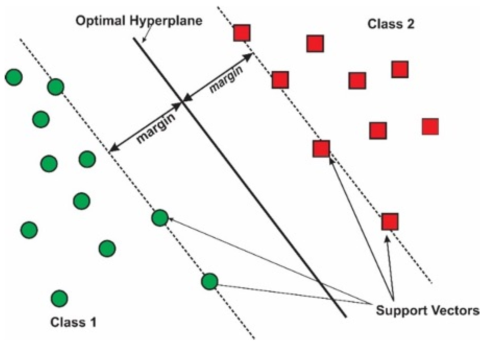
The SVM was proposed by Vapnik to classify data using the two dimensional space, as depicted in Figure 1.

If there is a dataset of $N$ points $\left(x_i,y_i\right)$, where $i$ ranges from $1 \mathrm{t}\mathrm{o} N$, $x_i$ represents the input data, and $y_{i }\in \left\{-\mathrm{1,1}\right\}$ denotes the class label. SVM aims to find the optimal hyperplane that maximizes the margin between the classes. This optimal hyperplane maximizes the distance between itself and the closest data points of each class.

$$Minimize {\displaystyle \frac{1}{2}}{‖w‖}^2+C\sum _{i=1}^n{\xi }_i$$

(17)

This is subjected to $y_i\left(w^T{x}_i+b\right)\ge 1-{\xi }_i \mathrm{a}\mathrm{n}\mathrm{d} {\xi }_i\ge 0 \mathrm{f}\mathrm{o}\mathrm{r} i=1 \mathrm{t}\mathrm{o} N$, where $w$ represents the weight vector, $b$ is the bias, $T$ denotes the transpose, and ${\xi }_i$ is the slack variable. The values of $w$ and $b$ are determined during the training process. The regularization parameter $C$ controls the model’s complexity by balancing the margin size and the number of misclassified points. A Lagrange multiplier, ${\alpha }_i$, is used to treat the hyperplane as a quadratic form. It incorporates constraints into the quadratic equation, transforming it into an unconstrained problem. The parameter $w$ is derived from Ref. [22]. The objective function of SVM is defined in Equation (18).

$$w\left(\alpha \right)=\sum _{i=1}^n{\alpha }_i\mathrm{ }+{\displaystyle \frac{1}{2}}\sum _{i,j=1}^n{\alpha }_i{\alpha }_j{x}_i{y}_{i}k\left(x_i,x_j\right)$$

(18)

where ${\alpha }_i,{\alpha }_j$ are the Lagrange multiplier and ${k(x}_i,x_j)$ is the kernel function.

$$f=sign(b+{\sum }_{SV}\left[{(\alpha }_i{y}_i\left)k\right(x_i,x_j)\right])$$

(19)

A positive Lagrange multiplier indicates that the corresponding data point is a SV. The kernel function enables the computation of dot products in feature space without explicitly mapping the input data into that space. Many kernel functions are available, and

Table 1. Different kernel function [21].

Kernel Function	Formula
Linear	$k\left(x_i,x_j\right)=x_i.x_j$
Polynomial	$k\left(x_i,x_j\right)={\left(\gamma x_i.x_j+r\right)}^d, \gamma >0$
Radian basis function (RBF)	$k\left(x_i,x_j\right)=\mathrm{e}\mathrm{x}\mathrm{p}(-\gamma {‖x_i-x_j‖}^2), \gamma >0$
Sigmoid	$k\left(x_i,x_j\right)=tanh\left(\gamma x_i.x_j+r\right)$

provides a list of some of the most widely used.

The regularization parameter ($C$) and kernel parameter (γ) significantly influence the SVM performance. Selecting an appropriate value for $C$ minimizes misclassification by maximizing the margin and reducing the training error. A large $C$ value leads to low bias but can cause overfitting, while a small $C$ value may result in high bias and underfitting. Therefore, C should be chosen carefully. In this study, the radial basis function (RBF) kernel (parameterized by γ) was used to transform the input data into a higher-dimensional space, which helps control the sharpness of peaks in the decision boundary. A smaller γ value creates sharper peaks, and a larger value produces smoother peaks. The COA was employed to optimize both $C$ and γ in this work. Traditional MATLAB optimization methods like grid search and Bayesian optimization can also be used, but they are often time-consuming. The search ranges for $C$ and γ, based on Ref. [21], are presented in

Table 2. The search range of SVM parameters [21].

Parameter	Setting
C	0.1–5
γ	100–1000

.

3. Proposed Work

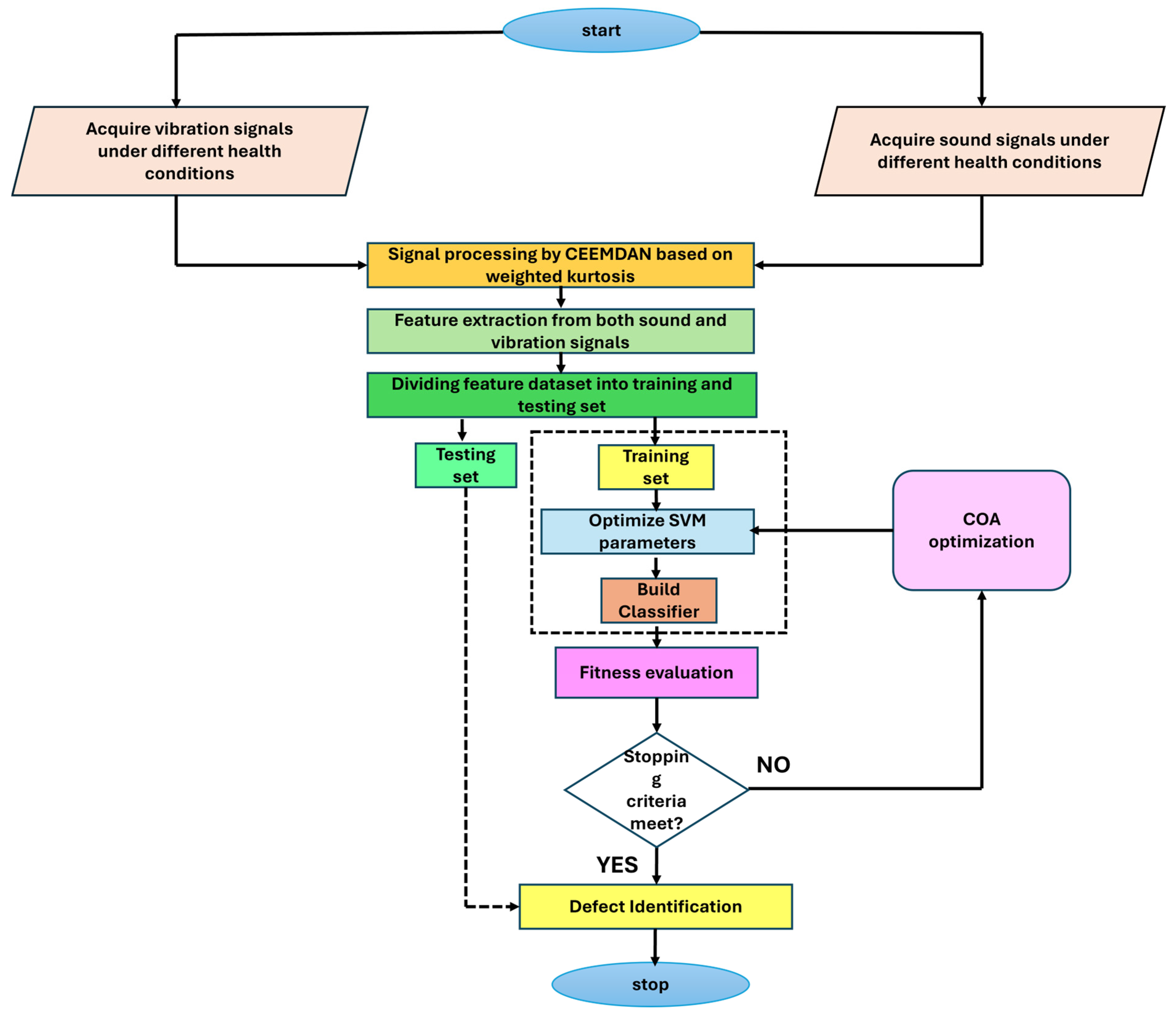
The detailed steps for the proposed work are given below and are also represented in Figure 2.

• Acquire the multi-sensor data from the centrifugal pump under different health conditions.
• Process the raw signals through CEEMDAN to obtain the IMFs.
• Compute the weighted kurtosis for each IMF to identify the significant IMFs based on their maximum value.
• Extract the features from multi-domains (i.e., time domain, frequency domain, and time–frequency domain).
• Prepare the dataset after applying the feature-level fusion technique.
• Normalize the dataset and further divide it into the training and testing datasets in the ratio 70:30.
• The SVM parameters are optimized through COA to improve the recognition rate.
• Validation of the built model should be carried out.

4. Application of the Proposed Methodology

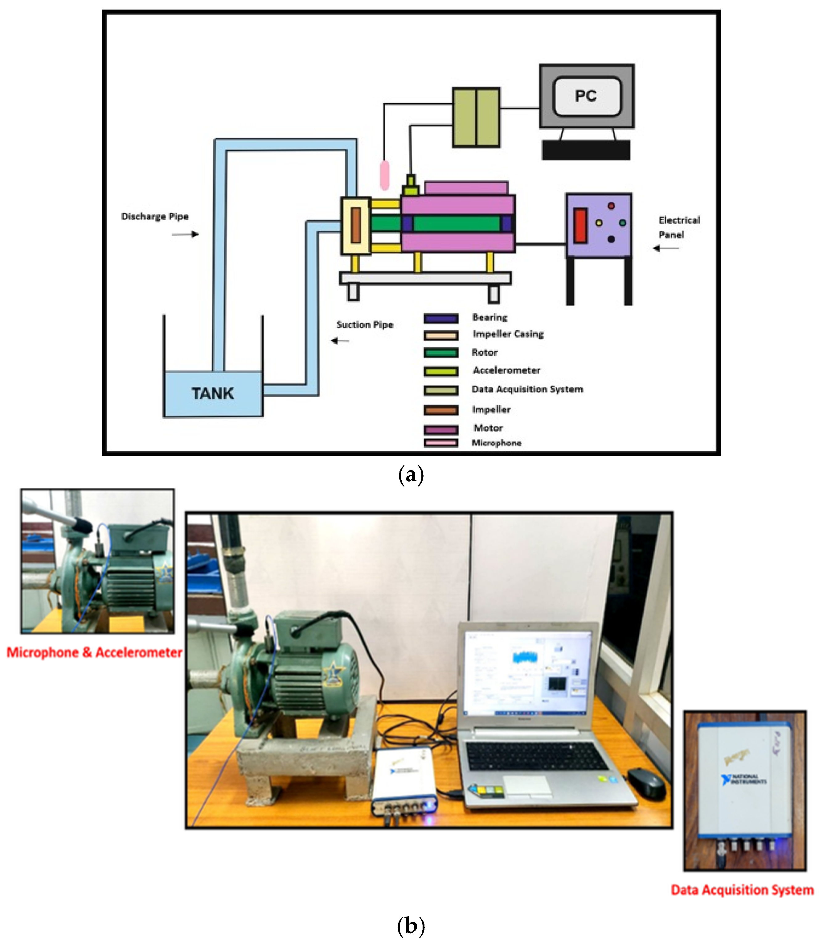
For this experiment, a monoblock centrifugal pump was utilized to identify impeller defects. The specifications of the centrifugal pump are tabulated in

Table 3. Specifications of the centrifugal pump [23].

Power supply	230/240 V
Motor power	0.5 HP
Discharge	1.61 L/s
Impeller type	Closed
Impeller diameter, impeller vanes	118.88 mm, 3

. Figure 3 illustrates the schematic and typical image of the test rig, which incorporated a sound sensor and data acquisition equipment. The pump was operated at a constant speed of 2800 RPM, resulting in an operating frequency of 46.67 Hz. The test rig’s rotor shaft was supported by two bearings: Bearing 1 (bearing number 6203-ZZ), which was positioned closer to the impeller, and Bearing 2 (bearing number 6202-ZZ), located farther from the impeller. The impeller itself was situated on the rotor shaft and enclosed within the pump casing. It consists of rotating vanes that draw water axially through the impeller’s eye. The vanes then impart kinetic energy to the water, forcing it to flow radially outward through the casing. The interaction between the water and the rotating vanes, specifically the energy transfer through impacts, is what generates the chaotic phenomena within the water flow.

A uniaxial PCB accelerometer with a sensitivity of 100 mV/g was used to capture the vibration signals. The accelerometer was attached to the impeller casing using wax, as shown in Figure 3. A National Instruments 24-bit DAQ system (Austin, TX, USA) with 4 channels, set to a sampling frequency of 70,000 Hz, acquired the signal. Simultaneously, a microphone with a sensitivity of −60 dB recorded the sound signal, also at a sampling frequency of 70,000 Hz.

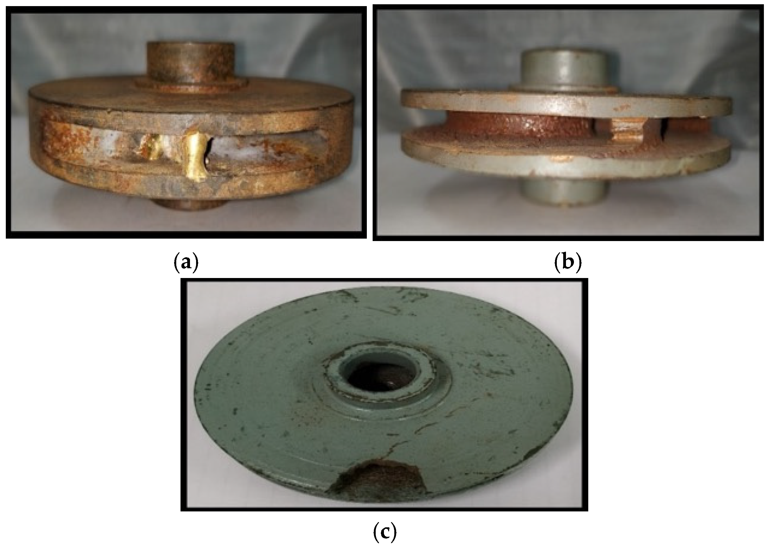
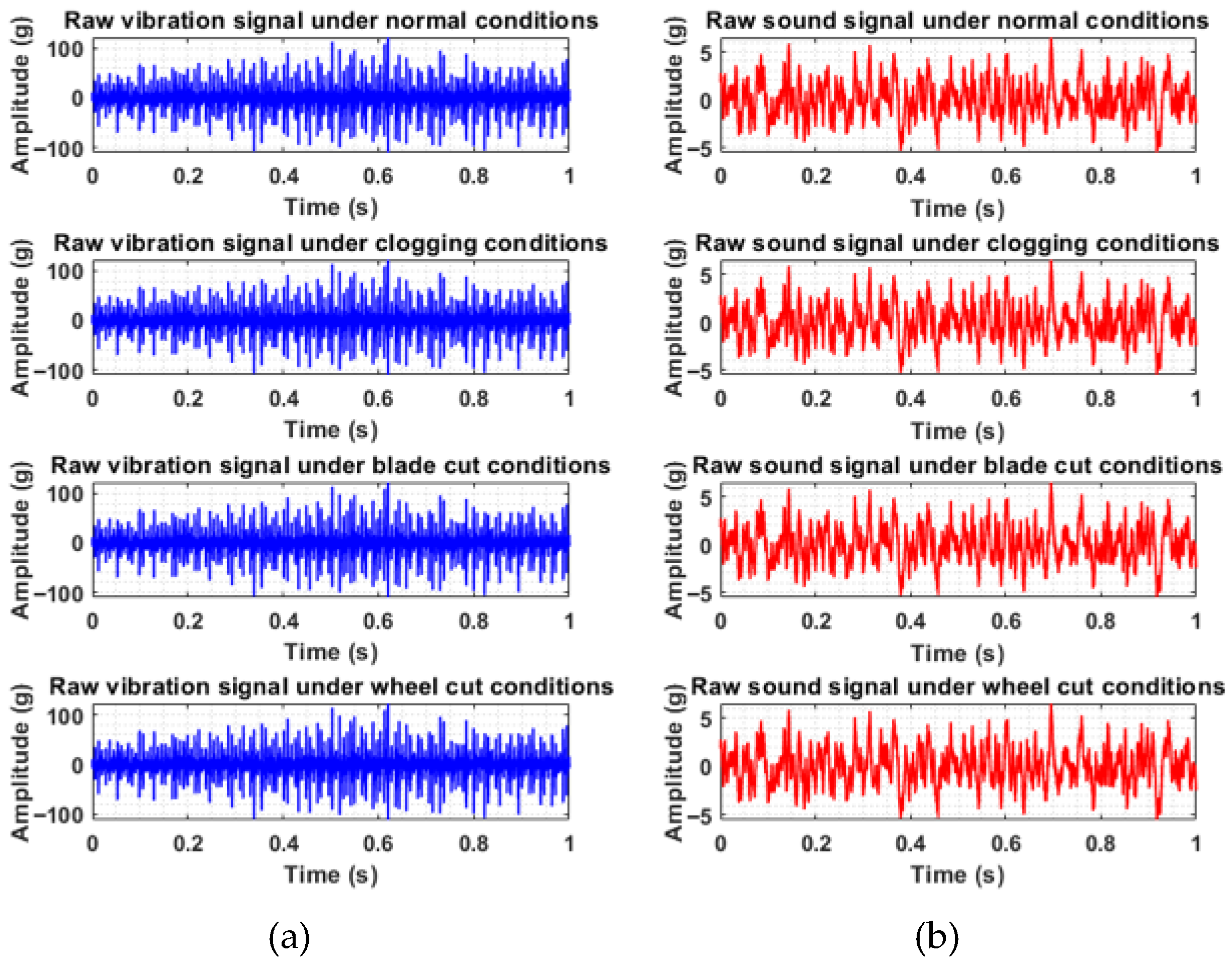
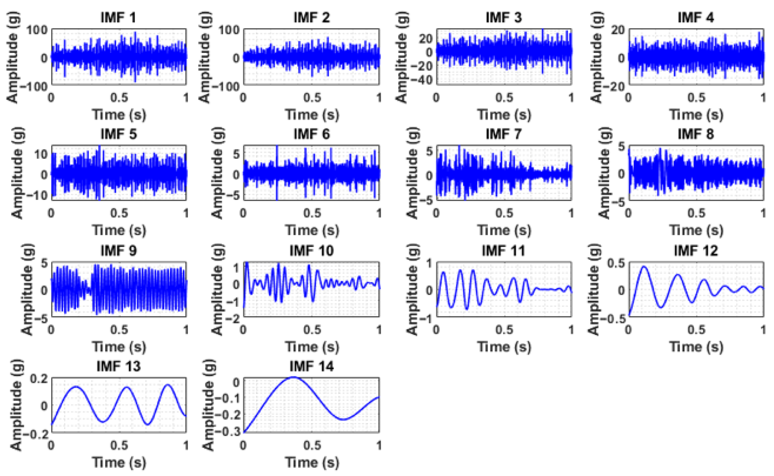
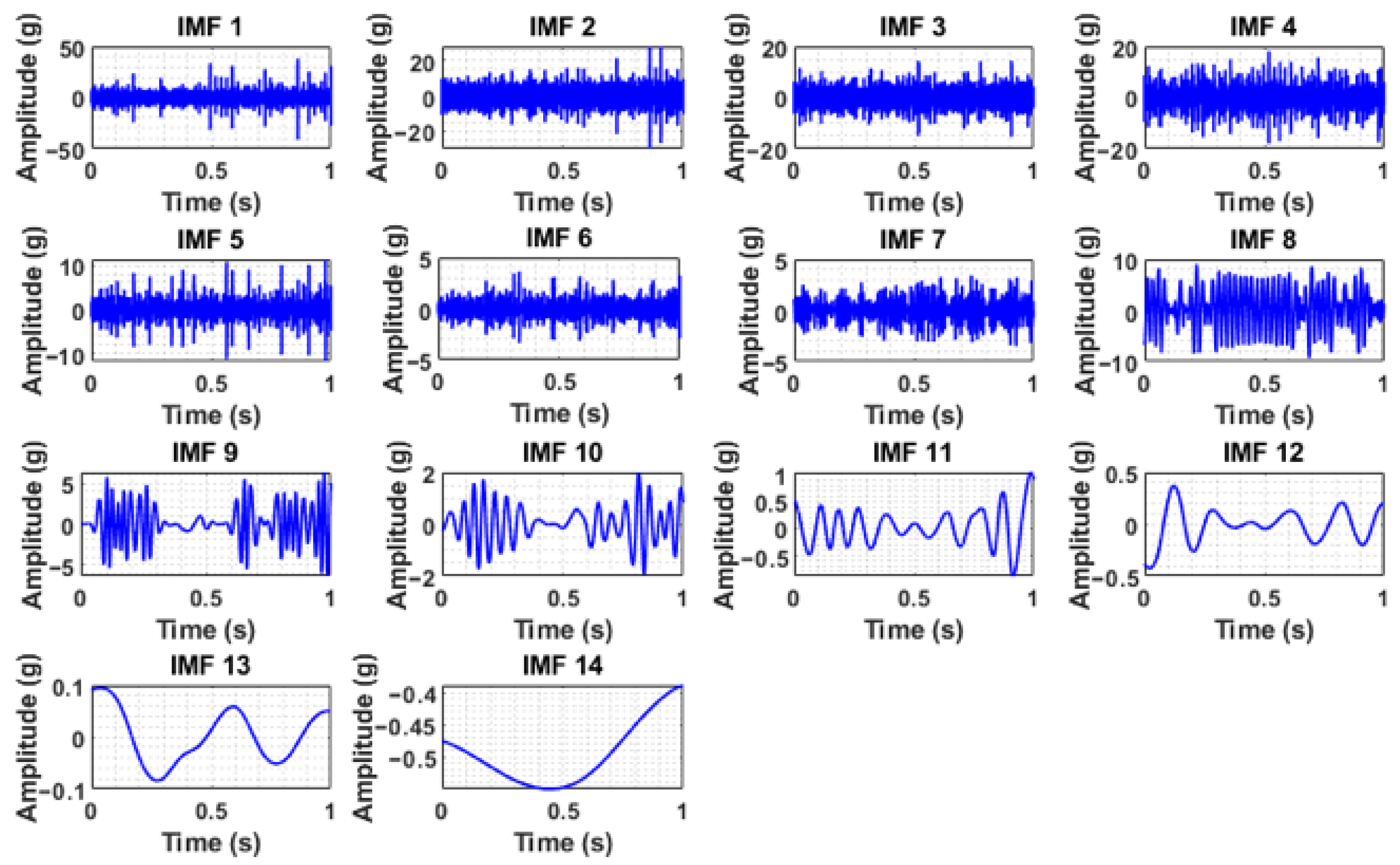
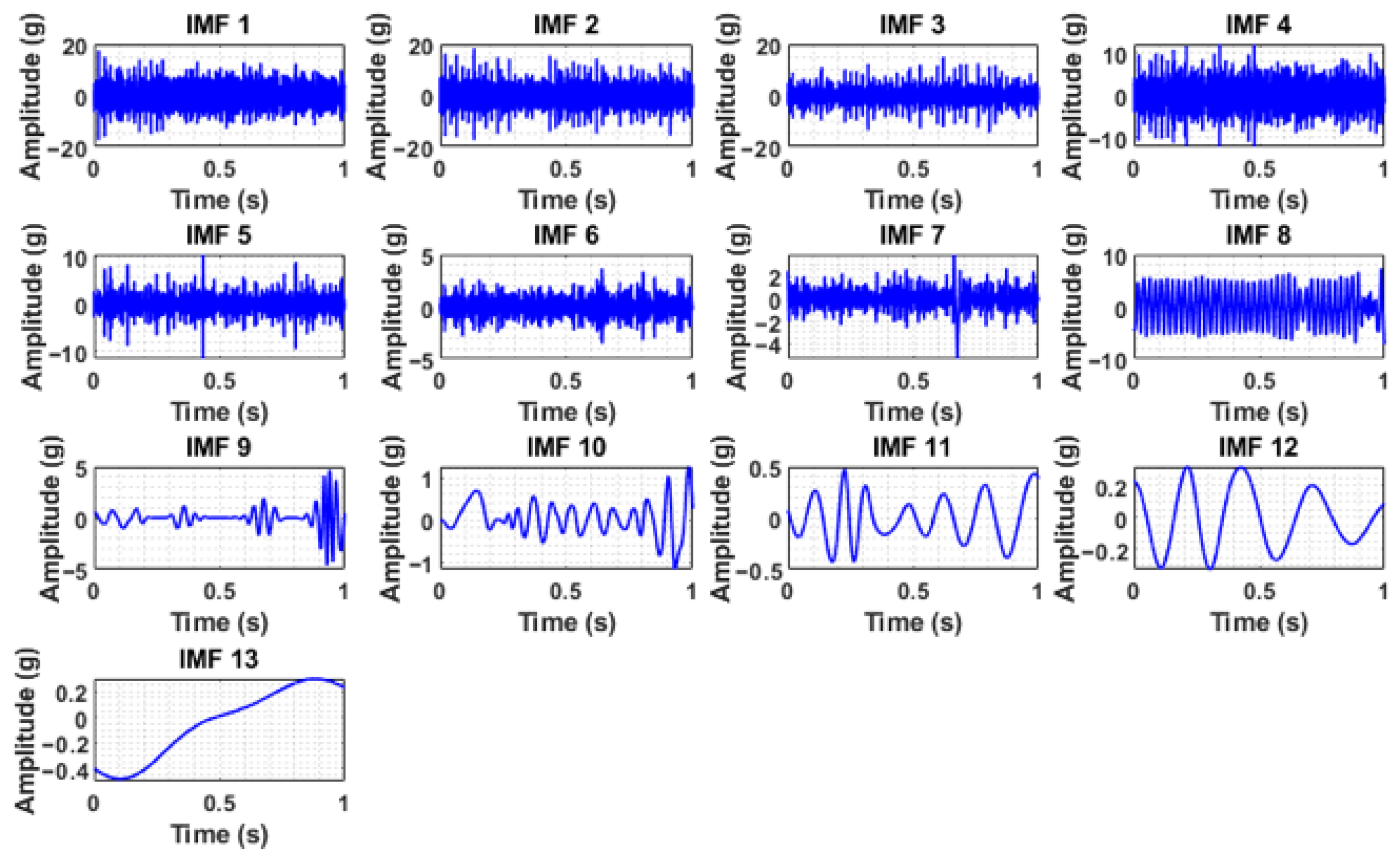
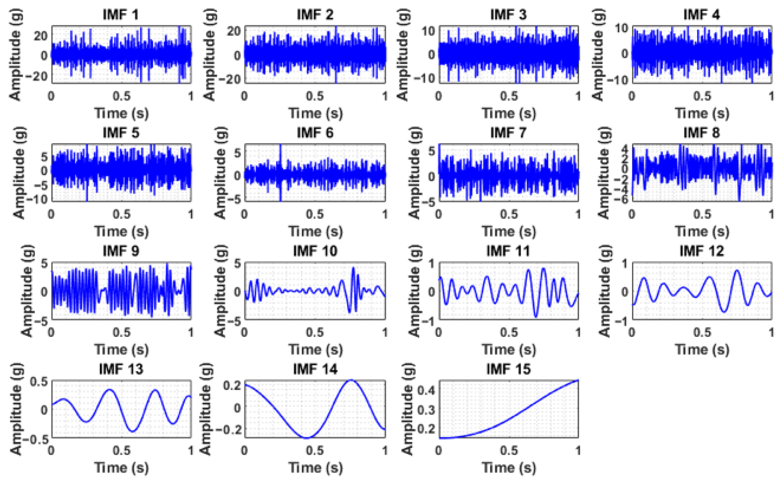
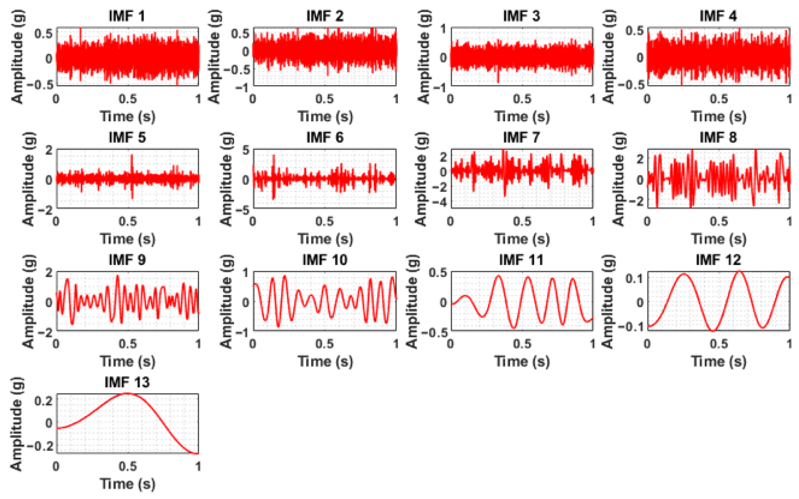
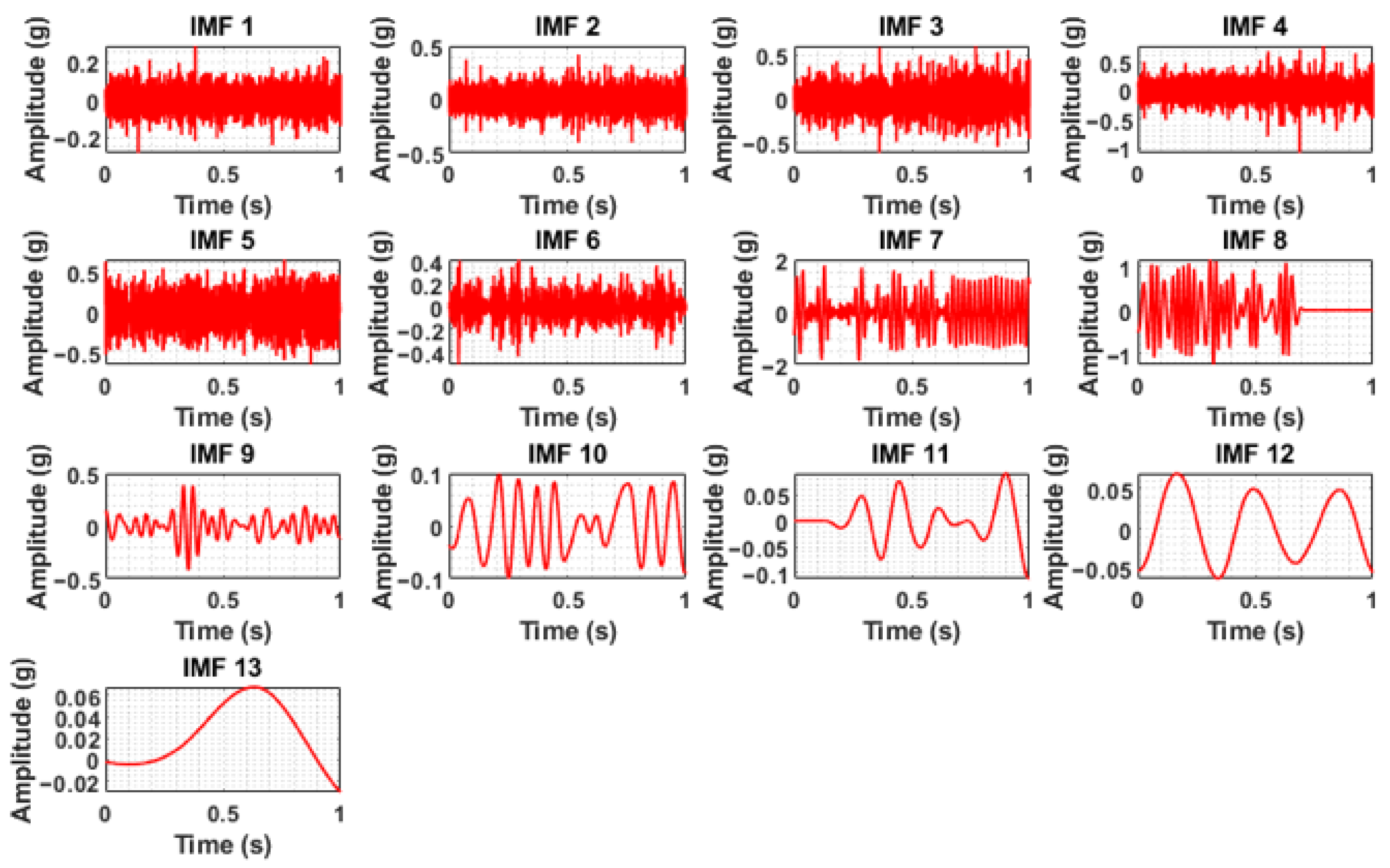
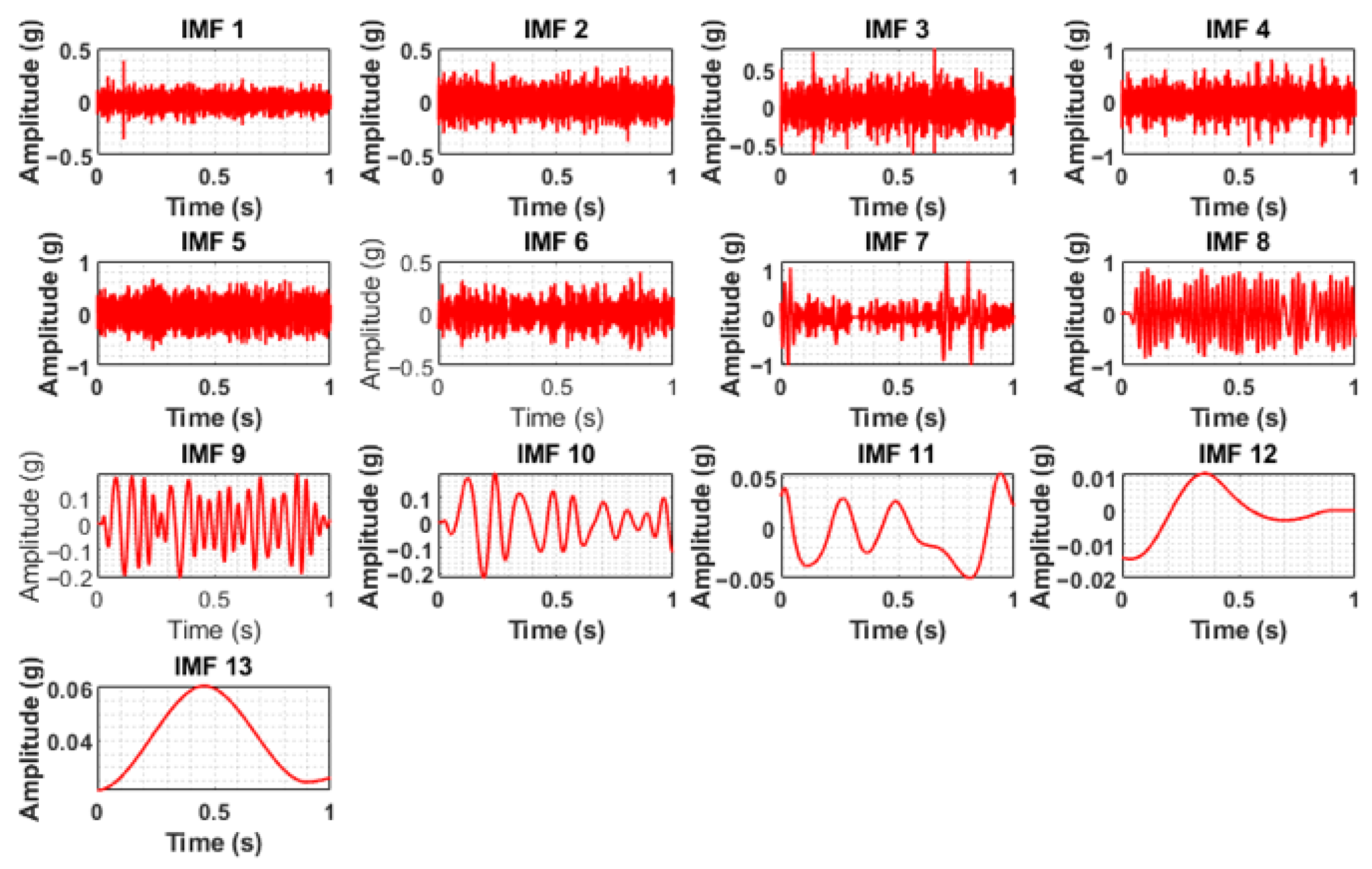
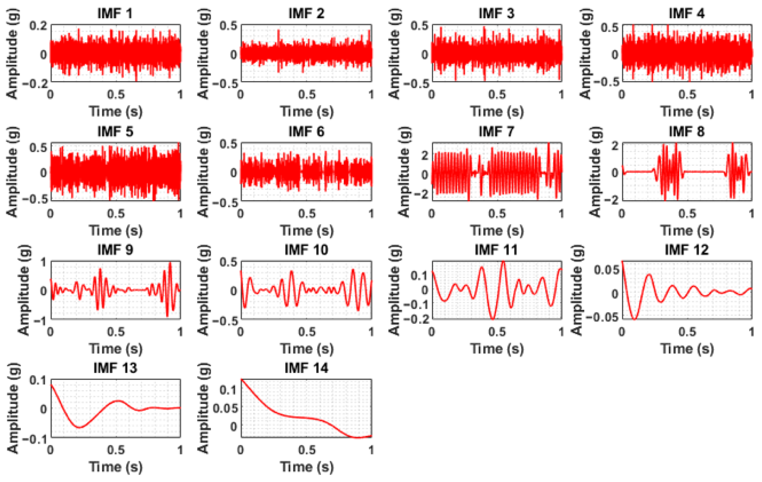
Four distinct health conditions were analyzed: healthy, clogging, blade cut, and wheel cut, as shown in Figure 4. The raw signals, displayed in Figure 5, are clearly masked with noise, necessitating preprocessing via complete ensemble empirical mode decomposition with adaptive noise (CEEMDAN). In the case of the normal condition, the vibration signal was more consistent and possibly had a lower amplitude, suggesting stable operation, whereas the sound signal during normal operation had background noise. In the case of clogging, the vibration signal showed slightly increased randomness or higher frequency components, potentially indicating turbulent flow or increased mechanical stress due to blockage. The sound signals also exhibited higher-frequency noise, which is associated with turbulent flow due to the blockage. The blade cut or wheel cut conditions showed some impulsive peaks or irregular patterns, reflecting impacts or imbalances caused by the damage in the vibration signals, whereas the acoustic data showed a distortion that represents the altered sound profile because of the blade cut and wheel cut. CEEMDAN decomposed the raw signals into various intrinsic mode functions (IMFs). The IMFs obtained by CEEMDAN under different health conditions for both the vibration signals and sound signals are shown in Figure 6, Figure 7, Figure 8, Figure 9, Figure 10, Figure 11, Figure 12 and Figure 13.

The IMFs containing useful information were considered significant and identified based on the maximum value of weighted kurtosis. The weighted kurtosis assesses the effectiveness of the decomposition results by combining standard kurtosis and the correlation coefficient. Standard kurtosis is highly dependent on the density distribution of impacts generated by a fault. Therefore, relying solely on maximum kurtosis can neglect impacts with large amplitudes but dispersed density distributions. While the correlation coefficient quickly determines the similarity between two signals, it is susceptible to noise from faulty components. To leverage the advantages of both indices, weighted kurtosis was developed, as shown in Equation (20).

$$KCI=KI.\left|C\right|$$

(20)

where $KI$ represents the kurtosis index for input signal $x\left(n\right)$ and is expressed as

$$KI={\displaystyle \frac{\frac{1}{N}{\sum }_{n=0}^{N-1}{x}^4\left(n\right)}{{\left(\frac{1}{N}\sum _{n=0}^{N-1}{x}^2\left(n\right)\right)}^2}}$$

(21)

Here, the length of the signal is given by $N$. Considering $E\left[.\right]$ as a mathematical expectation, the correlation $C$ between $x$ and $y$ is expressed as:

$$C= {\displaystyle \frac{E\left[\left(x-\overline{x}\right)\left(y-\overline{y}\right)\right]}{E\left[{\left(x-\overline{x}\right)}^2\right]E\left[{\left(y-\overline{y}\right)}^2\right]}}$$

(22)

The weighted kurtosis obtained from the IMFs of the vibration signals is tabulated in

Table 4. Weighted kurtosis for different modes for vibration signals.

Condition	M1	M2	M3	M4	M5	M6	M7	M8	M9	M10	M11	M12	M13	M14	M15
Normal	11.3446	8.2567	3.1916	1.1590	1.0678	0.2911	0.4902	0.3253	0.3688	0.1097	0.0040	6.7294 × 10−4	3.4007 × 10−4	0.0015	-
Blade cut	5.7086	2.3391	1.4886	2.2290	1.4190	0.3116	0.5053	1.1249	0.7711	0.0010	0.0025	0.0112	0.0054	0.0065	0.0078
Clogging	2.9248	2.1873	2.5112	1.6482	1.2310	0.3507	0.4895	0.9998	0.2879	0.0356	0.0035	0.0071	0.0057	-	-
Wheel cut	6.6399	3.4269	1.6305	1.8405	1.5298	0.5381	0.6563	0.9274	0.6066	0.0193	0.0101	0.0278	0.0023	0.0086	0.0020

. Similarly, the weighted kurtosis obtained from the IMFs of the sound signals is presented in

Table 5. Weighted kurtosis for different modes for acoustic signals.

Condition	M1	M2	M3	M4	M5	M6	M7	M8	M9	M10	M11	M12	M13
Normal	0.2736	0.3754	0.3100	0.3266	1.3614	2.3960	1.8352	1.6788	1.0321	0.7588	0.1297	0.1232	0.0049
Blade cut	0.2752	0.4271	0.7323	0.9714	0.5812	0.5629	1.8599	1.7116	0.0375	0.0745	0.0411	0.0141	0.0032
Clogging	0.4923	0.5470	1.1804	1.2899	0.8410	0.5112	2.3472	1.3757	0.3560	0.2534	0.1468	0.0264	0.0353
Wheel cut	0.1736	0.2454	0.2743	0.3237	0.3691	0.2017	1.8553	1.4669	0.1737	0.0203	0.0903	0.0281	0.0543

.

The analysis of the weighted kurtosis values, as presented in the accompanying tables, revealed that a substantial portion of the IMFs exhibited very small kurtosis values. This observation suggests that these IMFs contribute negligibly to the overall signal, indicating a lack of meaningful information content. Consequently, these IMFs were deemed unsuitable for subsequent analysis and excluded from further consideration. To ensure the selection of the most informative components, the top five significant IMFs were chosen based on the maximum weighted kurtosis values derived from both the vibration and sound signals for each defined health condition. This selection process prioritized IMFs that captured the most prominent characteristics related to the health status of the system under investigation.

Following the identification of these significant IMFs, a comprehensive set of 30 features, detailed in

Table 6. Features from the time domain, frequency domain, and time–frequency domain.

Feature Notation and Formula	Feature Notation and Formula	Feature Notation and Formula
Mean A1 = ${\displaystyle \frac{1}{N}}{\sum }_{i=1}^N{x}_i$	Kurtosis A11 $={\displaystyle \frac{1}{{\sigma }^4}}\left({\displaystyle \frac{1}{N-1}}{\sum }_{i=1}^N{\left(x_i-\mu \right)}^4\right)$	Median absolute deviation A21 = $median\left(\right|x_i-median\left(x_i\right)\left|\right)$
Root mean square A2 = $\sqrt{{\displaystyle \frac{1}{N}}{\sum }_{i=1}^N{x}_i^2}$	Crest factor A12 $={\displaystyle \frac{max\left(\left|x\right|\right)}{\sqrt{\frac{1}{N}{\sum }_{i=1}^N{x}_i^2}}}$	Rate zero crossing A22 = ${\displaystyle \frac{number of zero crossings}{total number of points}}$
Root A3 = ${\left({\displaystyle \frac{1}{N}}{\sum }_{i=1}^N\sqrt{\left|x_i\right|}\right)}^2$	Shape factor A13 $={\displaystyle \frac{\sqrt{\frac{1}{N}{\sum }_{i=1}^N{x}_i^2}}{\frac{1}{N}{\sum }_{i=1}^N{|x}_i|}}$	Entropy A23 $=-\sum _{1=1}^{N}h\left(x_i\right){\log }_{2}h\left(x_i\right)$
Maximum value A4 = $max\left(\left|x\right|\right)$	Impulse factor A14 $={\displaystyle \frac{max\left(\left|x\right|\right)}{\frac{1}{N}{\sum }_{i=1}^N{|x}_i|}}$	Histogram upper bound A24 $=max\left(x_i\right)+{\displaystyle \frac{max\left(x_i\right)-min\left(\frac{x_i}{N-1}\right)}{2}}$
Peak-to-peak A5 = $max\left(\left|x\right|\right)-min\left(\left|x\right|\right)$	Clearance factor A15 $={\displaystyle \frac{max\left(\left|x\right|\right)}{{\left(\frac{1}{N}{\sum }_{i=1}^N\sqrt{\left|x_i\right|}\right)}^2}}$	Histogram lower bound A25 $=max\left(x_i\right)-{\displaystyle \frac{max\left(x_i\right)-min\left(\frac{x_i}{N-1}\right)}{2}}$
Standard deviation A6 = $\sqrt{{\displaystyle \frac{1}{N-1}}{\sum }_{i=1}^N{\left(x_i-\mu \right)}^2}$	Skewness factor A16 $= {\displaystyle \frac{1}{{\sigma }^3}}{\displaystyle \frac{\left(\frac{1}{N-1}{\sum }_{i=1}^N{\left(x_i-\mu \right)}^3\right)}{{\left(\sqrt{\frac{1}{N}{\sum }_{i=1}^N{x}_i^2}\right)}^2}}$	Activity A26 $={\displaystyle \frac{1}{N-1}}{\sum }_{i=1}^N{\left(x_i-\mu \right)}^2$
Median A7 = ${\displaystyle \frac{50(N+1)}{100}}th observation$	Kurtosis factor A17 $= {\displaystyle \frac{1}{{\sigma }^4}}{\displaystyle \frac{\left(\frac{1}{N-1}{\sum }_{i=1}^N{\left(x_i-\mu \right)}^4\right)}{{\left(\sqrt{\frac{1}{N}{\sum }_{i=1}^N{x}_i^2}\right)}^4}}$	Variance A27 $={\displaystyle \frac{{\sum }_{i=1}^N{(x\left(i\right)-x_{avg})}^2}{N-1}}$
25th Percentiles A8 = ${\displaystyle \frac{25(N+1)}{100}}th observation$	Geometric mean A18 $= {\left({\prod }_{i=N}^N{x}_i\right)}^{{\displaystyle \raisebox{1ex}{$1$}\!\left/ \!\raisebox{-1ex}{$N$}\right.}}$	Wavelet energy decomposition A28 $={\displaystyle \frac{{\sum }_{n=1}^N{\left|x_i\left(n\right)\right|}^2}{{\sum }_{k=0}^{2^j-1}{\sum }_{n=1}^N{\left|x_k\left(n\right)\right|}^2}}$
75th Percentiles A9 = ${\displaystyle \frac{75(N+1)}{100}}th observation$	Root sum of squares A19 $= \sqrt{{\sum }_{i=1}^N{\left|x_i\right|}^2}$	Normal negative log likelihood for single Gaussian A29 $=-\sum _{i=1}^{N}log\left[{\displaystyle \frac{1}{\sigma \sqrt{2\pi }}}exp{\displaystyle \frac{-{\left(x_i-\mu \right)}^2}{2{\sigma }^2}}\right]$
Skewness A10 $={\displaystyle \frac{1}{{\sigma }^3}}\left({\displaystyle \frac{1}{N-1}}{\sum }_{i=1}^N{\left(x_i-\mu \right)}^3\right)$	Mean absolute deviation A20 $=mean\left(\left|x_i-\mu \right|\right)$	Total harmonic distortion A30 = ${\displaystyle \frac{\sqrt{{\sum }_{i=2}^N{Y}_i^2}}{Y_i}}$

, were extracted from these selected components. This feature set encompassed a diverse range of descriptors drawn from the time domain, frequency domain, and time–frequency domain, providing a multi-faceted representation of the underlying signal characteristics. The combination of these features aims to capture both the temporal dynamics and spectral properties of the IMFs, enabling a more thorough and robust analysis of the system’s health condition.

The 30 features extracted from the significant IMFs of the vibration and sound signals, corresponding to each health condition, underwent a normalization process to ensure consistent scaling. Specifically, each feature was scaled to fall within the range of [0, 1]. This normalization step is crucial for preventing features with larger magnitudes from dominating the analysis and ensuring that all features contribute equally to subsequent modeling stages. Following normalization, the features derived from both the vibration and sound signals were fused, creating a unified dataset that integrated information from both sensor modalities. This fusion process resulted in a final dataset with dimensions of $40\times 30$, where the 40 rows represent the number of signal instances collected (i.e., 40 signals), and the 30 columns represent the total number of normalized features extracted from the significant IMFs. This combined dataset served as the input for further analysis and modeling.

To proceed with the classification of different health conditions, a support vector machine (SVM) was employed. It is well-known that the performance of an SVM, specifically its classification and prediction accuracy, is significantly influenced by the appropriate selection of its regularization parameter $\left(C\right)$ and kernel function parameter (γ). An arbitrary or random selection of these parameters can lead to suboptimal results. Indeed, the results of the initial classification attempts using arbitrarily chosen values for $C$ and γ, as presented in Table 5, demonstrated a poor recognition rate and a time-consuming optimization process. Therefore, it is crucial to optimize the selection of these parameters to design an efficient and accurate SVM model. In this study, the parameters $C$ and γ were optimized using the CAO as described in Section 2.2. The CAO algorithm was configured with a population size of 30, and the optimization process was terminated when a maximum of 100 iterations was reached. All processing and simulations were conducted using MATLAB R2024b running on a Windows 11 operating system with an Intel Core-i7 processor @2.30 GHz and 64 GB of RAM.

To ensure the robustness and generalizability of the SVM model and to avoid overfitting or underfitting, a $k-fold$ cross-validation technique was implemented during the classification process. $K-fold$ cross-validation involves partitioning the training dataset into k equal subsets or “folds.” During each iteration, $k-1$ folds are used for training the SVM model, while the remaining kth fold is used for validation. In this specific implementation, a $10-fold$ cross-validation technique was employed. The fitness of the SVM model was evaluated by calculating the cross-validation error, as defined by Equation (23). This error metric guides the CAO in its search for the optimal $C$ and γ parameters, aiming to minimize the cross-validation error and maximize the model’s predictive performance.

$$Error={\displaystyle \frac{Number of samples incorrectly predicted while cross-validation}{Total number of training samples used for validation of accuracy}}\times 100\%$$

(23)

$$Accuracy=1-Error$$

(24)

The optimized SVM model achieved a classification accuracy of 95.0%. The computational cost associated with optimizing the SVM parameters using the proposed algorithm and training the SVM model was 22.7249 s. The optimized values for the regularization parameter C and the kernel function parameter γ, which yielded the maximum accuracy, were determined to be 3.1258 and 512.9957, respectively.

Table 7. Effectiveness of SVM at different values of C and γ.

S. No.	C Value	γ Value	Efficiency
1	4.127	189.9128	62.67%
2	3.2598	499.8147	79.87%
3	2.4179	522.1742	80.60%
4	3.1258	512.9957	95.0%

presents the performance of the SVM model using different combinations of C and γ, highlighting the impact of parameter selection on classification accuracy.

The efficacy of the proposed methodology was further assessed through the construction of a confusion matrix, as depicted in Figure 14. This matrix provides a detailed breakdown of the classification results, illustrating the number of instances correctly and incorrectly classified for each health condition. Analysis of the confusion matrix revealed that the proposed methodology effectively distinguished between different health conditions, achieving an overall classification accuracy of 95.0%. This demonstrates the ability of the system to accurately diagnose the state of the centrifugal pump.

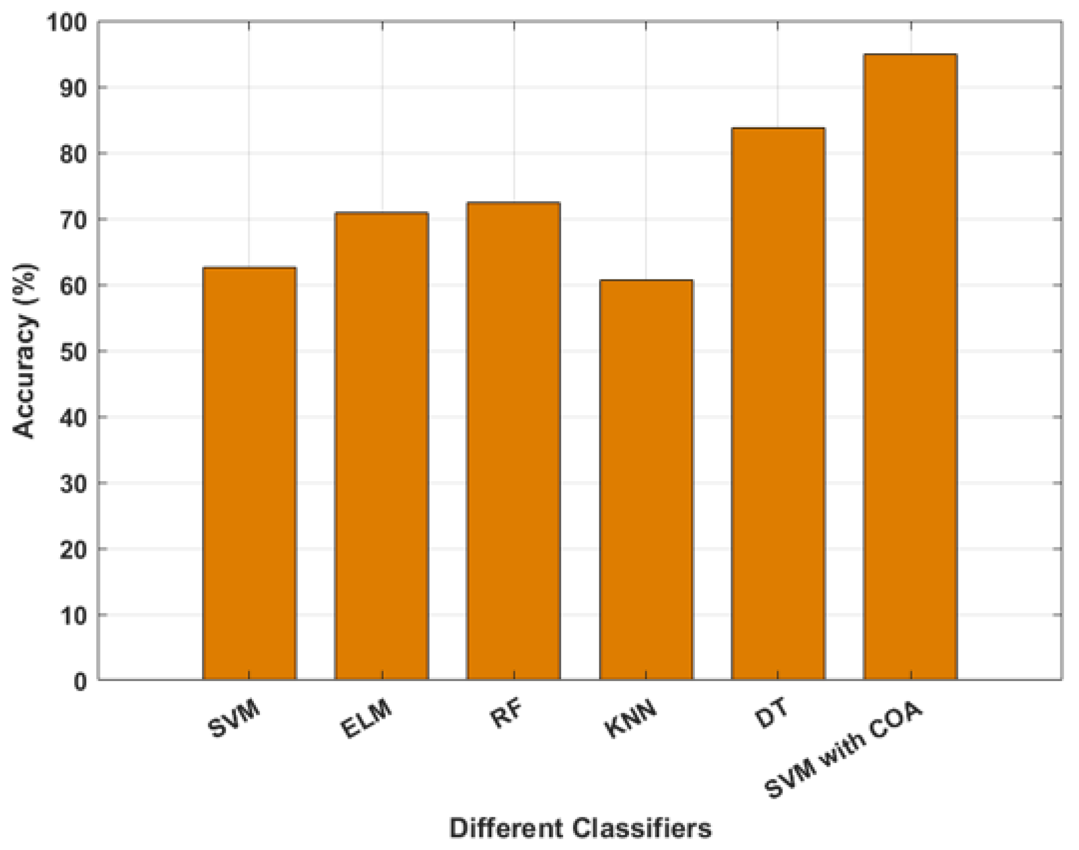
In order to validate the effectiveness of the proposed classifier, a comparative analysis was conducted against several established classification algorithms including a basic support vector machine (SVM), extreme learning machine (ELM), random forest (RF), k-nearest neighbor (k-NN), and decision tree (DT). The classification accuracies achieved by each of these algorithms were meticulously recorded and are presented visually in the bar plot in Figure 15. A detailed examination of Figure 15 revealed that the proposed method, specifically SVM optimized with the COA algorithm, demonstrated a superior level of accuracy compared with all of other classifiers evaluated. This significant performance advantage underscores the efficacy and potential of the proposed SVM with COA approach for the classification task under consideration.

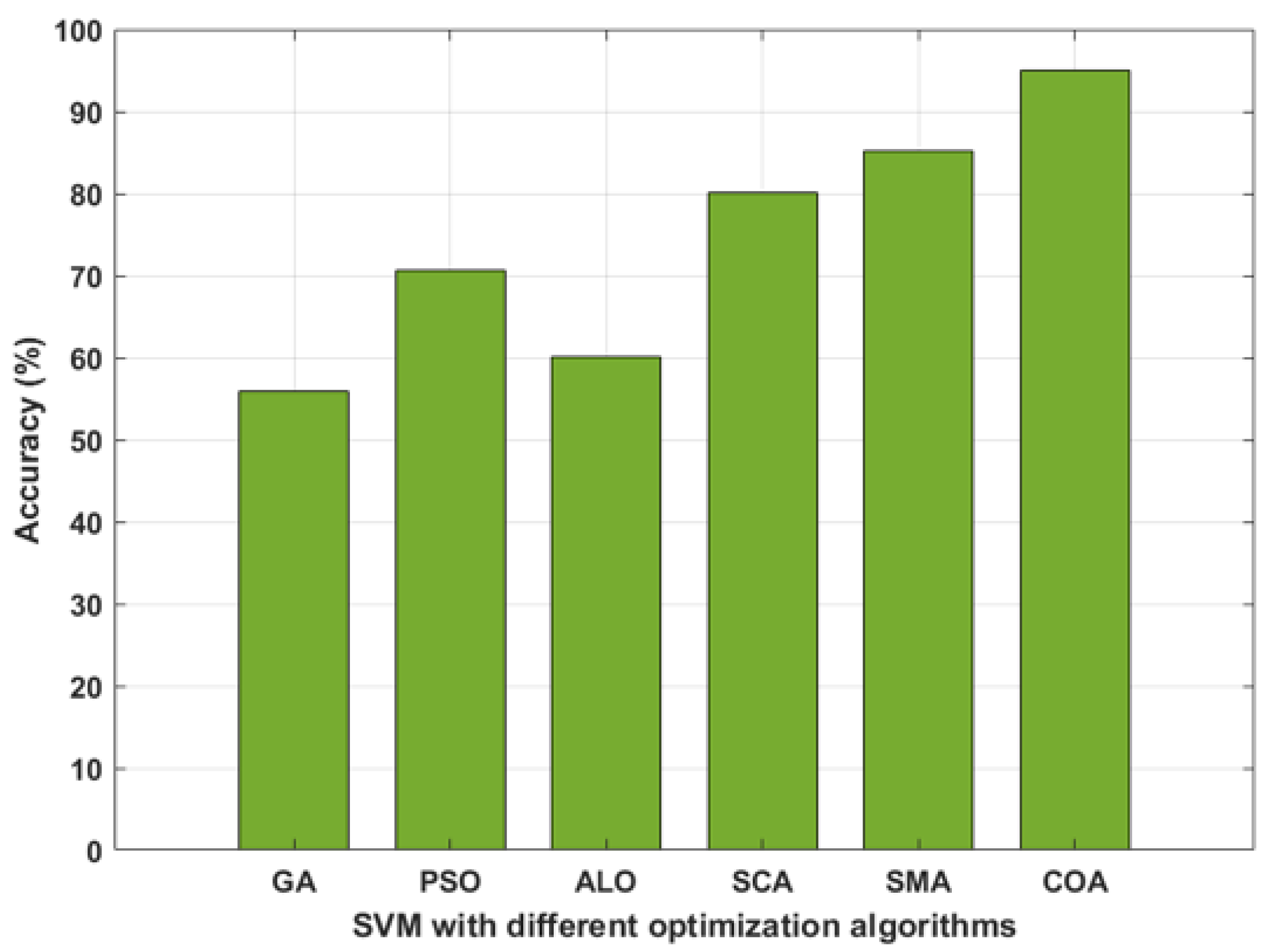
To further assess the effectiveness of the proposed methodology, a comprehensive comparison was undertaken against a range of well-established optimization algorithms. These included genetic algorithm (GA), particle swarm optimization (PSO), ant lion optimization (ALO), sine-cosine algorithm (SCA), and slime mold algorithm (SMA). The classification accuracies resulting from the application of each of these optimization algorithms are presented in detail in Figure 16. Upon the careful examination of Figure 16, it became evident that the proposed methodology achieved the highest level of accuracy in comparison to all of the other optimization algorithms tested. This clearly demonstrates the superior performance and potential of the proposed methodology for the given task.

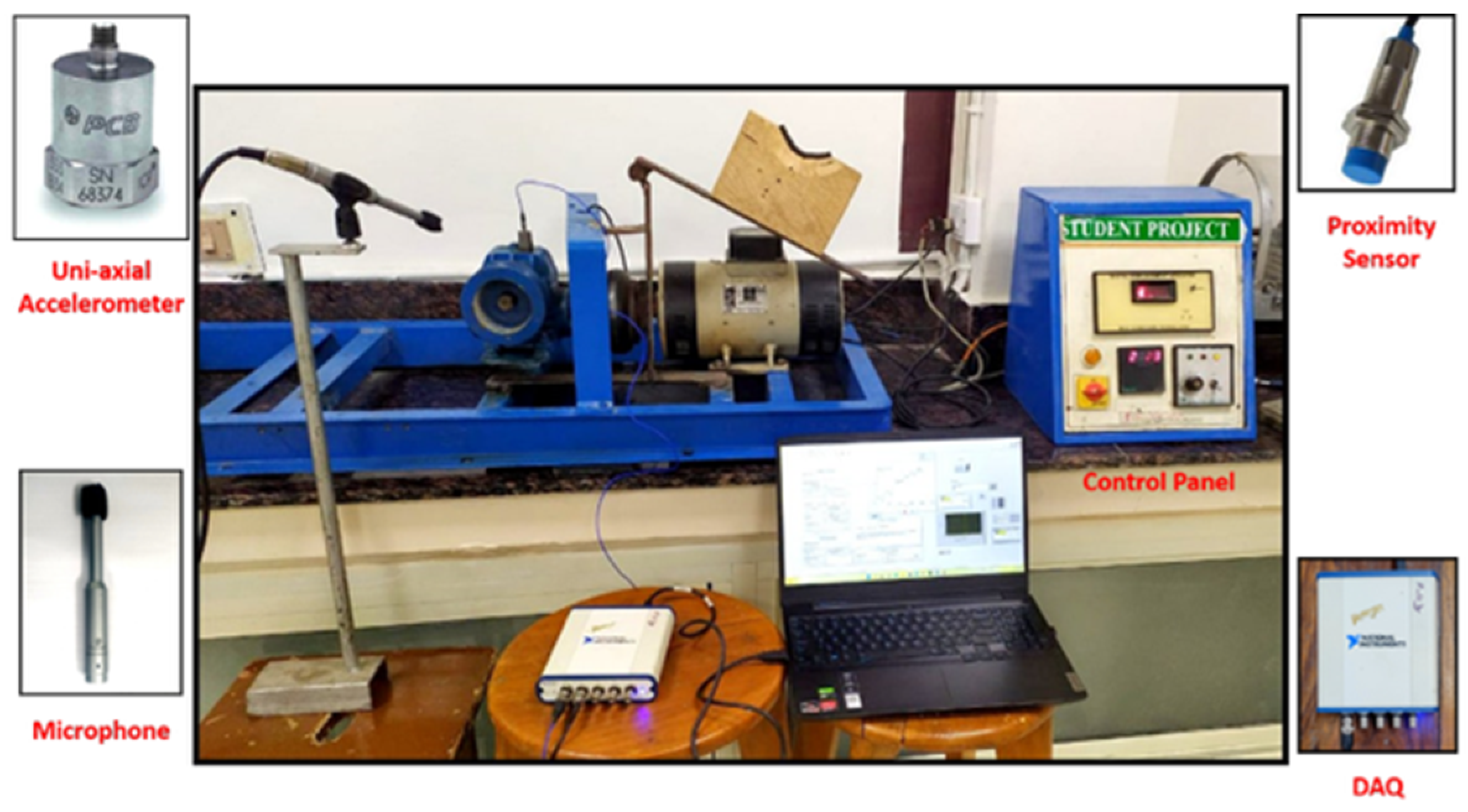
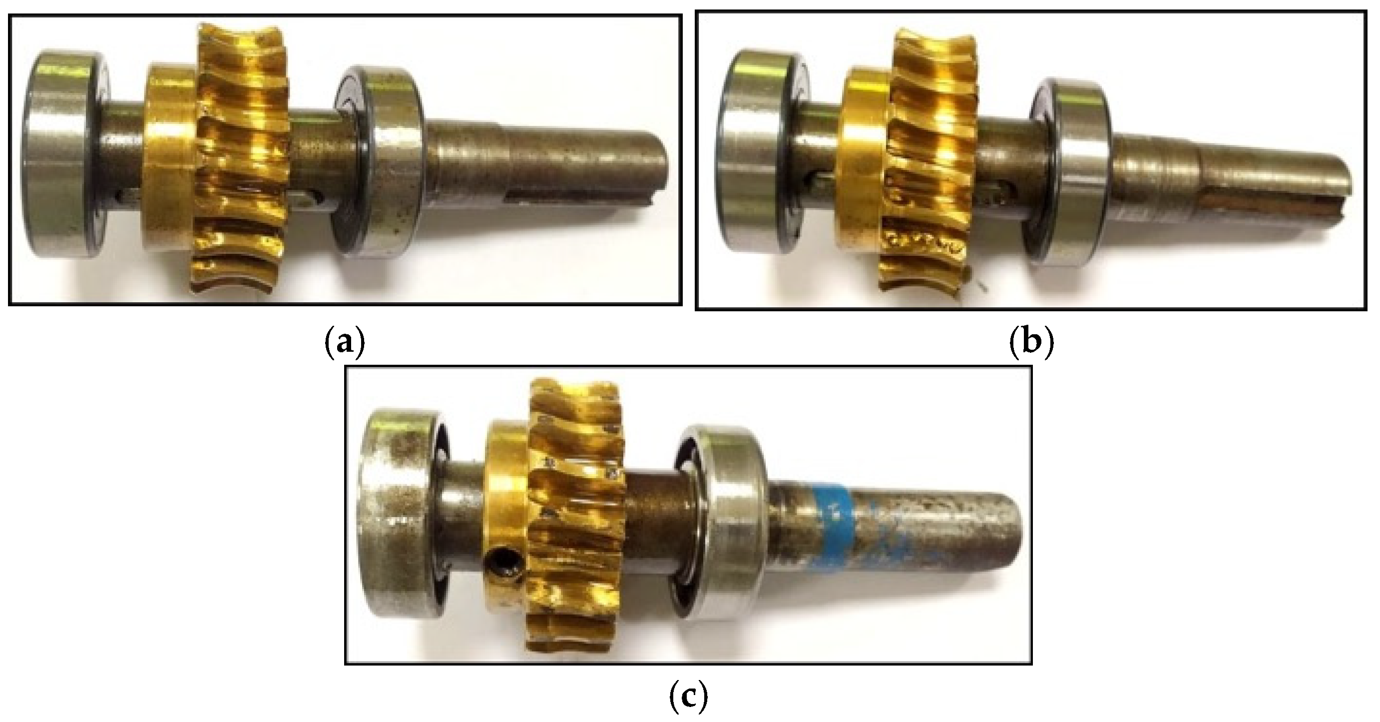
To ensure the robustness and generalizability of the proposed methodology, it was applied to a physical test rig of a worm gearbox. This gearbox was driven by a 50 Hz DC motor, with a flexible coupling connecting the two. The DC motor’s operation was governed by a control panel, as illustrated in Figure 17. Vibration and acoustic signals were acquired from the worm gearbox under three distinct health conditions, all tested at a rated RPM of 1500. The three health conditions considered were: healthy (representing a gearbox with no defects), pitting (representing a gearbox with surface fatigue), and missing (representing a gearbox with a missing tooth or component), as depicted in Figure 18. This approach allowed for a realistic evaluation of the methodology’s performance under varying operational scenarios.

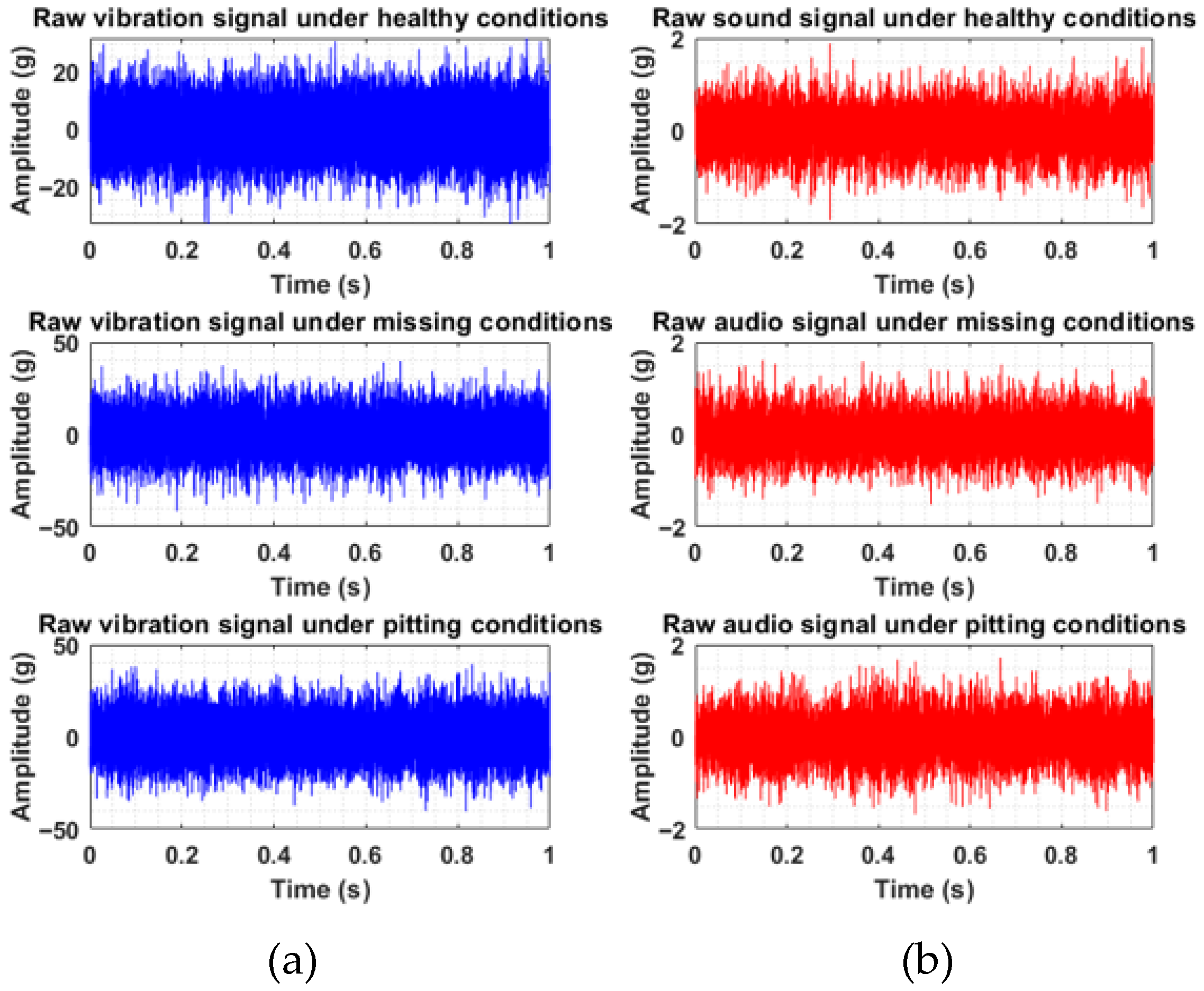
Initially, the worm within the gearbox was free of any intentionally introduced defects, representing the “healthy” operating condition. While this condition was considered the baseline, the potential for inherent, pre-existing flaws was acknowledged. For each of the three defined health conditions (healthy, pitting, and missing), signals were acquired while the gearbox operated at its rated RPM of 1500. Vibration data were captured using a PCB^® Piezotronics uniaxial accelerometer, characterized by a sensitivity of 100 mV/g. This accelerometer was directly mounted onto the gearbox housing to capture representative vibration patterns. Simultaneously, acoustic signals were recorded using an ECM 8000 microphone, exhibiting a sensitivity of −60 dB. A National Instruments DAQ system, featuring 24-bit resolution and 4-channel capability, was employed to acquire the vibration signals within the LabView 2020 environment. Subsequent analysis of the acquired data was performed using MATLAB R2019a software running on a machine configured with an AMD Ryzen 5 4600H processor with Radeon graphics (3 GHz), 8 GB of RAM, and a 64-bit Windows 10 operating system. The raw vibration and sound signals acquired during testing are presented in Figure 19.

In the case of the wormgear box, the optimized SVM model demonstrated a recognition accuracy of 97.2579%, achieved with a computation time of 20.5842 s. The optimized values for the regularization parameter C and the kernel function parameter γ, which yielded this high accuracy, were determined to be 3.5713 and 479.5685, respectively. Based on the results of both case studies, it can be inferred that the proposed method exhibits superior performance in accurately identifying different classes and possesses the potential for broad application across a variety of other domains.

5. Conclusions

This paper presents a robust and effective methodology for diagnosing faults in centrifugal pumps, leveraging the strengths of CEEMDAN and feature-level fusion. By integrating acoustic and vibration signals, the approach overcomes the limitations of traditional single-sensor methods, offering a more comprehensive and accurate assessment of pump health. The use of CEEMDAN for signal decomposition effectively addresses the challenges posed by non-stationary and noisy data, enabling the extraction of meaningful features. The selection of significant IMFs based on weighted kurtosis further enhances the diagnostic performance, while feature-level fusion ensures that complementary information from different sensors is effectively combined. The optimized SVM classifier, trained using the COA algorithm, achieved a high classification accuracy of 95.0%, demonstrating the practical applicability of the proposed methodology for real-world fault diagnosis. The SVM classifier, optimized using the COA, was evaluated against a range of alternative classifiers and optimization algorithms. Furthermore, it was also applied to a dataset acquired from a worm gearbox. The results demonstrate that the proposed method not only achieves superior accuracy, but also exhibits strong generalization capabilities, indicating its robustness and potential for broader application. This work provides a valuable contribution to the field of condition monitoring, offering a reliable tool for proactively identifying faults and preventing costly downtimes in centrifugal pump systems.

Finally, future studies could investigate the use of transfer learning techniques to adapt the trained model to different pump configurations and operating conditions, reducing the need for extensive retraining. These efforts would contribute to the development of more intelligent and efficient condition monitoring systems for rotating machinery, ultimately improving operational reliability and reducing the maintenance costs.

References

1. Rapur, J.S.; Tiwari, R. On-Line Time Domain Vibration and Current Signals Based Multi-Fault Diagnosis of Centrifugal Pumps Using Support Vector Machines. J. Nondestruct. Eval. 2018, 38, 6. [Google Scholar] [CrossRef]
2. Vashishtha, G.; Kumar, R. Unsupervised Learning Model of Sparse Filtering Enhanced Using Wasserstein Distance for Intelligent Fault Diagnosis. J. Vib. Eng. Technol. 2023, 11, 2985–3002. [Google Scholar] [CrossRef]
3. Jiang, L.; Du, H.; Bu, Y.; Zhao, C.; Lu, H.; Yan, J. Deep Learning-Based Multilabel Compound-Fault Diagnosis in Centrifugal Pumps. Ocean Eng. 2024, 314, 119697. [Google Scholar] [CrossRef]
4. Ahmad, S.; Ahmad, Z.; Kim, J.-M. A Centrifugal Pump Fault Diagnosis Framework Based on Supervised Contrastive Learning. Sensors 2022, 22, 6448. [Google Scholar] [CrossRef]
5. ALTobi, M.A.S.; Bevan, G.; Wallace, P.; Harrison, D.; Ramachandran, K.P. Fault Diagnosis of a Centrifugal Pump Using MLP-GABP and SVM with CWT. Eng. Sci. Technol. Int. J. 2019, 22, 854–861. [Google Scholar] [CrossRef]
6. Ali, M.Z.; Shabbir, M.N.S.K.; Liang, X.; Zhang, Y.; Hu, T. Machine Learning-Based Fault Diagnosis for Single- and Multi-Faults in Induction Motors Using Measured Stator Currents and Vibration Signals. IEEE Trans. Ind. Appl. 2019, 55, 2378–2391. [Google Scholar] [CrossRef]
7. Cai, B.; Liu, Y.; Fan, Q.; Zhang, Y.; Liu, Z.; Yu, S.; Ji, R. Multi-Source Information Fusion Based Fault Diagnosis of Ground-Source Heat Pump Using Bayesian Network. Appl. Energy 2014, 114, 1–9. [Google Scholar] [CrossRef]
8. Fu, Y.; Chen, X.; Liu, Y.; Son, C.; Yang, Y. Multi-Source Information Fusion Fault Diagnosis for Gearboxes Based on SDP and VGG. Appl. Sci. 2022, 12, 6323. [Google Scholar] [CrossRef]
9. Azizi, R.; Attaran, B.; Hajnayeb, A.; Ghanbarzadeh, A.; Changizian, M. Improving Accuracy of Cavitation Severity Detection in Centrifugal Pumps Using a Hybrid Feature Selection Technique. Measurement 2017, 108, 9–17. [Google Scholar] [CrossRef]
10. Xu, Y.; Wang, H.; Xu, F.; Bi, S.; Ye, J. A Sensor Data-Driven Fault Diagnosis Method for Automotive Transmission Gearboxes Based on Improved EEMD and CNN-BiLSTM. Processes 2025, 13, 1200. [Google Scholar] [CrossRef]
11. Shi, J.; Hou, Y.; Wang, Z.; Yang, Z.; Lv, Z. A Diagnostic Method for Noise and Intermittent Faults in Analog Circuits Based on the EEMD-SR Filtering Algorithm and LSTM-CM. Measurement 2025, 254, 117871. [Google Scholar] [CrossRef]
12. Duan, N.; Zeng, Y.; Dao, F.; Xu, S.; Luo, X. Fault Diagnosis of Hydro-Turbine Based on Ceemdan-Mpe Preprocessing Combined with Cpo-Bilstm Modelling. Energies 2024, 18, 1342. [Google Scholar] [CrossRef]
13. Li, J.; He, D.; Wei, Z.; Zhao, M.; Xiang, Z. CEEMDAN and Adaptive Distance Embedding for Fault Diagnosis of Train Bogie Bearing. Meas. Sci. Technol. 2025, 36, 036127. [Google Scholar] [CrossRef]
14. Ouelaa, Z.; Djebala, A.; Younes, R.; Chaabi, L.; Ouelaa, N.; Bouacha, K.; Mrabti, A. Advanced Gear Fault Diagnosis in Non-Stationary Conditions with an Improved CEEMDAN-Wavelet Denoising Technique. Adv. Mech. Eng. 2025, 17, 16878132251356546. [Google Scholar] [CrossRef]
15. Zhang, T.; Sun, H. A Method for Predicting the Remaining Life of Lithium-Ion Batteries Based on an Improved Dempster–Shafer Evidence Theory Framework. Energies 2025, 18, 3370. [Google Scholar] [CrossRef]
16. Hou, Y.; Wang, J.; Chen, Z.; Ma, J.; Li, T. Diagnosisformer: An Efficient Rolling Bearing Fault Diagnosis Method Based on Improved Transformer. Eng. Appl. Artif. Intell. 2023, 124, 106507. [Google Scholar] [CrossRef]
17. Hou, Y.; Li, T.; Wang, J.; Ma, J.; Chen, Z. A Lightweight Transformer Based on Feature Fusion and Global–Local Parallel Stacked Self-Activation Unit for Bearing Fault Diagnosis. Measurement 2024, 236, 115068. [Google Scholar] [CrossRef]
18. Lv, Y.; Yuan, R.; Wang, T.; Li, H.; Song, G. Health Degradation Monitoring and Early Fault Diagnosis of a Rolling Bearing Based on CEEMDAN and Improved MMSE. Materials 2018, 11, 1009. [Google Scholar] [CrossRef] [PubMed]
19. Torres, M.E.; Colominas, M.A.; Schlotthauer, G.; Flandrin, P. A Complete Ensemble Empirical Mode Decomposition with Adaptive Noise. In Proceedings of the 2011 IEEE International Conference on Acoustics, Speech and Signal Processing (ICASSP), Prague, Czech Republic, 22–27 May 2011; pp. 4144–4147. [Google Scholar]
20. Jia, H.; Rao, H.; Wen, C.; Mirjalili, S. Crayfish Optimization Algorithm. Artif. Intell. Rev. 2023, 56, 1919–1979. [Google Scholar] [CrossRef]
21. Chauhan, S.; Vashishtha, G.; Gupta, M.K.; Korkmaz, M.E.; Demirsöz, R.; Noman, K.; Kolesnyk, V. Parallel Structure of Crayfish Optimization with Arithmetic Optimization for Classifying the Friction Behaviour of Ti-6Al-4V Alloy for Complex Machinery Applications. Knowl. Based Syst. 2024, 286, 111389. [Google Scholar] [CrossRef]
22. Chauhan, S.; Singh, M.; Kumar Aggarwal, A. An Effective Health Indicator for Bearing Using Corrected Conditional Entropy through Diversity-Driven Multi-Parent Evolutionary Algorithm. Struct. Health Monit. 2020, 20, 2525–2539. [Google Scholar] [CrossRef]
23. Vashishtha, G.; Chauhan, S.; Yadav, N.; Kumar, A.; Kumar, R. A Two-Level Adaptive Chirp Mode Decomposition and Tangent Entropy in Estimation of Single-Valued Neutrosophic Cross-Entropy for Detecting Impeller Defects in Centrifugal Pump. Appl. Acoust. 2022, 197, 108905. [Google Scholar] [CrossRef]
Figure 1. Basic architecture of SVM [21].
Algorithms 18 00644 g001
Figure 2. Flowchart of the proposed methodology.
Algorithms 18 00644 g002
Figure 3. (a) Schematic of the test rig and (b) pictorial view of the test rig [23].
Algorithms 18 00644 g003
Figure 4. Different operating conditions. (a) Clogging, (b) blade cut, and (c) wheel cut [23].
Algorithms 18 00644 g004
Figure 5. Raw signals of centrifugal pump under different health conditions. (a) Left panel showing vibration signals. (b) Right panel showing sound signals.
Algorithms 18 00644 g005
Figure 6. IMFs obtained by CEEMDAN of the vibration signal under the normal condition.
Algorithms 18 00644 g006
Figure 7. IMFs obtained by CEEMDAN of the vibration signal under the clogging condition.
Algorithms 18 00644 g007
Figure 8. IMFs obtained by CEEMDAN of the vibration signal under the blade cut condition.
Algorithms 18 00644 g008
Figure 9. IMFs obtained by CEEMDAN of the vibration signal under the wheel cut condition.
Algorithms 18 00644 g009
Figure 10. IMFs obtained by CEEMDAN of the sound signal under the normal condition.
Algorithms 18 00644 g010
Figure 11. IMFs obtained by CEEMDAN of the sound signal under the clogging condition.
Algorithms 18 00644 g011
Figure 12. IMFs obtained by CEEMDAN of the sound signal under the blade cut condition.
Algorithms 18 00644 g012
Figure 13. IMFs obtained by CEEMDAN of the sound signal under the wheel cut condition.
Algorithms 18 00644 g013
Figure 14. Confusion matrix.
Algorithms 18 00644 g014
Figure 15. Comparison of accuracy with different classifiers.
Algorithms 18 00644 g015
Figure 16. Comparison of the accuracy of the proposed method with different optimization algorithms.
Algorithms 18 00644 g016
Figure 17. Worm gearbox test rig.
Algorithms 18 00644 g017
Figure 18. Health states of worm gearbox. (a) Healthy, (b) pitting, and (c) missing.
Algorithms 18 00644 g018
Figure 19. Raw signals for worm gearbox under different health conditions. (a) Left panel showing vibration signals. (b) Right panel showing sound signals.
Algorithms 18 00644 g019