Abstract
Rolling bearing vibration signals are often severely affected by strong external noise, which can obscure fault-related features and hinder accurate diagnosis. To address this challenge, this paper proposes an enhanced Deep Residual Shrinkage Network with Dynamic Convolution and Selective Kernel Attention (DDRSN-SKA). First, one-dimensional vibration signals are converted into two-dimensional time frequency images using the Continuous Wavelet Transform (CWT), providing richer input representations. Then, a dynamic convolution module is introduced to adaptively adjust kernel weights based on the input, enabling the network to better extract salient features. To improve feature discrimination, an Selective Kernel Attention (SKAttention) module is incorporated into the intermediate layers of the network. By applying a multi-receptive field channel attention mechanism, the network can emphasize critical information and suppress irrelevant features. The final classification layer determines the fault types. Experiments conducted on both the Case Western Reserve University (CWRU) dataset and a laboratory-collected bearing dataset demonstrate that DDRSN-SKA achieves diagnostic accuracies of 98.44% and 94.44% under −8 dB Gaussian and Laplace noise, respectively. These results confirm the model’s strong noise robustness and its suitability for fault diagnosis in noisy industrial environments.
1. Introduction
Bearings are widely used in industrial applications such as aerospace, automotive manufacturing, and wind power generation [1]. Once a bearing fails, it can cause severe equipment damage or even safety accidents. Therefore, developing efficient and accurate methods for bearing fault diagnosis is of great practical importance [2,3,4].
Traditional fault diagnosis approaches primarily rely on signal processing and machine learning techniques, including the Fourier Transform [5], Wavelet Transform [6], and Support Vector Machine [7]. Although these methods are capable of identifying bearing faults to a certain extent, they suffer from significant drawbacks, including a strong reliance on manual feature extraction, high sensitivity to noise, and poor generalization to unseen conditions [8]. These drawbacks make it challenging to apply them effectively in noisy industrial environments. To address these issues, researchers have proposed various improvements to traditional methods. For instance, Xie et al. [9] combined fractional-order Fourier transform with lightweight neural networks, while Shen et al. [10] introduced a fault diagnosis method based on SVM optimized by a gray wolf algorithm. Although these approaches have improved diagnostic accuracy to a degree [11]. They still rely on handcrafted features and expert knowledge, leading to high subjectivity and limited generalization capability [12].
Unlike traditional methods, deep learning methods can automatically learn abstract representations of data features from input signals, convolutional neural networks (CNNs) [13] has become an especially important tool for state identification of mechanical equipment due to its strong automatic feature extraction capability and end-to-end modeling advantages. Therefore, more and more researchers have introduced CNNs into bearing fault diagnosis tasks [14]. For example, Wang et al. [15] proposed a VBICNN model by combining variational Bayesian inference with a CNN, which significantly improves the accuracy and stability of diagnosis through a multi-sensor data fusion strategy. Xu et al. [16] designed an improved parallel CNN structure using a multi-branch convolutional layer instead of the traditional pooling layer, which enhances the feature extraction capability and improves the generalization ability of the model under variable loads. Although the above improved CNN model has achieved some success in bearing fault diagnosis, it still has some limitations in dealing with strong noise interference conditions [17]. First, the CNN model lacks an intrinsic denoising mechanism and is easily affected by strong noise, leading to distortion of feature extraction [18]. Second, although the multi-channel structure enhances the feature expression, it significantly increases the model complexity, decreases the training efficiency, and is prone to overfitting [19]. In addition, although they introduce an attention mechanism to enhance robustness, some methods have not effectively solved the problem of feature redundancy coexisting with noise [20].
In recent years, research in the field of machine health monitoring has moved beyond traditional fault diagnosis, showing two leading-edge trends. The first is a shift in focus from fault “diagnosis” to “prognosis”, which involves predicting the remaining useful life (RUL) of equipment. To achieve this, the academic community is exploring advanced signal processing and modeling techniques, such as enhanced particle filters [21] and cyclic spectral coherence [22], as well as cutting-edge machine learning architectures, like attention-guided graph isomorphism learning [23], that can capture complex system dependencies. The second trend, driven by the need to reduce cost and system complexity, is the emergence of techniques like sensorless robust anomaly detection using motor driver data [24], representing a move towards data fusion and non-invasive monitoring. Although these advanced prognostic and sensorless methods paint a broad future for the field, their effectiveness often relies on a core prerequisite: the ability to accurately and reliably identify incipient, weak fault features from noisy raw data.
To cope with the impact of noise on fault diagnosis, Deep Residual Shrinkage Network (DRSN) [25] has been proposed and gradually applied to bearing fault diagnosis tasks. By introducing a soft threshold shrinkage mechanism, this network effectively suppresses redundancy and strong noise information, while retaining the key fault features, and demonstrates better discriminative ability in strong noise environments. In recent years, researchers have carried out various optimizations of DRSN to enhance its usefulness. For example, Li et al. [26] proposed a method combining DRSN and Transformer model for bearing fault diagnosis, which maintains high accuracy under strong noise and effectively improves the model’s noise immunity and feature extraction ability. Li et al. [27] proposed a DRSN-GCE model, which effectively improves the noise immunity in bearing fault diagnosis by introducing gated convolution and a shrinkage mechanism. Li et al. [28] proposed the MSCMN-eDRSN model, which combines multi-scale convolution and nonlinear feature extraction to significantly improve the accuracy of fault diagnosis under strong noise. Wang et al. [29] introduced an improved soft threshold function and attention mechanism to enhance the local feature focus, but its convolutional structure still lacks the dynamic perception of time-varying features of the signal, which limits the model’s ability to detect the time-varying features perception. Chen et al. [30] proposed an adaptive multichannel residual shrinkage network (AMC-RSN), which enhances the feature expression and noise immunity through multichannel fusion and a soft thresholding module, but their method is still deficient in the dynamic adjustment of channel selection.
Inspired by the above approaches, this paper proposes a DDRSN-SKA algorithm for fault classification and identification of rolling bearings, as a research object for the cases that the vibration signal of the rolling shaft is easily affected by strong noise. The main contributions of this paper are as follows:
- (1)
- We propose a novel residual shrinkage network, DDRSN-SKA. By incorporating a dynamic convolution structure, the network adaptively generates convolution kernel weights according to the input signal, enabling more effective extraction of discriminative features from noisy vibration data. Compared with traditional fixed convolution kernels, the dynamic convolution greatly enhances feature representation. Furthermore, the SK attention mechanism adaptively selects appropriate receptive fields during convolution, thereby improving the recognition of critical fault features and further enhancing diagnostic accuracy.
- (2)
- We design an enhanced residual shrinkage unit that integrates dynamic convolution with Selective Kernel Attention (SKAttention) to strengthen feature extraction under strong noise conditions. While conventional residual shrinkage units possess denoising capability, they often attenuate or even lose key fault signatures when processing signals with high noise levels, particularly in weak fault or severely distorted cases. To address this, we replace conventional convolution with dynamic convolution, allowing for adaptive adjustment of kernel weights based on signal characteristics and significantly improving the model’s sensitivity to feature variations. In addition, SKAttention selectively emphasizes informative channel features, effectively enhancing the network’s ability to capture abnormal patterns. This structure not only preserves the denoising advantages of residual shrinkage units but also improves the retention of weak fault features, enabling robust fault recognition under complex operating conditions.
- (3)
- The effectiveness of the proposed method is validated on the Case Western Reserve University (CWRU) bearing dataset and a laboratory-collected bearing dataset. The Experimental results show that our model consistently outperforms baseline algorithms across different noise levels, confirming its robustness and superiority. In particular, under strong noise interference, the model effectively extracts and distinguishes fault patterns, demonstrating substantial potential for real-world engineering applications.
Based on the contents of the paper, we pose several scientific questions. How can reliable fault features be extracted from rolling bearing vibration signals heavily contaminated by Gaussian and Laplace noise? Under severe noise interference, how can critical diagnostic information be preserved? Can the integration of dynamic convolution (adaptive kernel weight adjustment) and SKAttention (multi-receptive-field channel weighting) into a deep residual shrinkage network enhance the ability to capture time-varying fault features and improve noise robustness? When evaluated on the CWRU dataset and laboratory-collected data, does the proposed DDRSN-SKA model significantly outperform existing advanced methods (e.g., ResNet, DRSN-CS, DRSN-Transformer), particularly under extremely low SNR conditions (e.g., −8 dB)?
The remainder of this paper is organized as follows. Section 2 introduces the theoretical foundation and architecture of DDRSN-SKA, including continuous wavelet transform (CWT), dynamic convolution, SKAttention, and the enhanced Residual Shrinkage Building Unit (DRSBU). Section 3 presents the experimental validation, covering the experimental setup, comparative and ablation studies on both datasets under different noise conditions, and performance analysis using confusion matrices and t-SNE visualization. Section 4 concludes the work by revisiting the scientific questions, highlighting the practical value and challenges of the proposed approach, and outlining future research directions.
2. Theoretical Foundations and Network Structure
This chapter will systematically elaborate on the theoretical foundations and network architecture of the DDRSN-SKA model, whose core components are constructed layer by layer around the goal of “extracting and enhancing fault features under strong noise”. Firstly, to address the issue of blurred features in one-dimensional vibration signals amid noise, Section 2.1 introduces the Continuous Wavelet Transform (CWT), which preserves richer time frequency domain information by converting signals into two-dimensional time frequency images. Building on this, Section 2.2 incorporates a dynamic convolution module that dynamically adjusts weights through a multi-convolution kernel weighting mechanism, enhancing the network’s adaptability to time-varying features in complex noisy environments. To further strengthen the discriminability of key features, Section 2.3 details the Selective Kernel Attention (SKAttention) mechanism, a module that suppresses redundant information via a multi-receptive field channel weighting strategy. Finally, Section 2.4 proposes an Enhanced Deep Residual Shrinkage Network (Enhanced DRSN), which integrates the aforementioned components into a unified architecture. Through the improved Residual Shrinkage Building Unit (DRSBU), it achieves the collaborative enhancement of noise robustness and feature extraction capability.
2.1. Continuous Wavelet Transform
The Wavelet Transform (WT) is a time frequency analysis tool that can provide information about a signal in both the time and frequency domains. Different from the traditional Fourier transform, Wavelet Transform has the ability of Multi-Resolution Analysis (MRA), which can effectively process non-stationary signals, and is very suitable for vibration signals, shock signals, and other transient changes in the engineering scenarios, and especially in the field of mechanical fault diagnosis is widely used. It obtains the spectral information of a signal at different scales and positions by convolving the signal with a set of wavelet basis functions. The wavelet basis functions correspond to typology (1).
The continuous wavelet transform corresponds to typology (2).
where , are continuously varying parameters, a is the scale parameter, b is the translation parameter, and and the wavelet basis function and are complex numbers to each other conjugate.
When performing the continuous wavelet transform (CWT), the selection of the wavelet basis functions has a key impact on the accuracy of signal feature extraction. Common wavelet basis functions include Morlet, Daubechies (e.g., Db10), Coiflet (e.g., Coif5), and Meyer. Among them, the Morlet wavelet is particularly good in rolling bearing fault diagnosis because of its good smoothness, symmetry, and modulation characteristics, which can more accurately locate the frequency components of faults and their positions in the time domain on the time frequency scale. Based on the above advantages, this paper selects the Morlet wavelet as the mother wavelet function in continuous wavelet transform. The Morlet wavelet can be calculated using expression (3).
where t is the time variable; is the angular frequency parameter, which generally takes a value between 5 and 6 to obtain a better time frequency localization effect; j is an imaginary unit.
2.2. Dynamic Convolution
Traditional convolutional layers employ fixed kernels that do not adapt to varying input characteristics, which limits their ability to extract meaningful features under complex and noisy conditions. To overcome this limitation, the proposed model incorporates a dynamic convolution mechanism that adjusts the contribution of multiple convolutional kernels based on the input features.
As illustrated in Figure 1, the dynamic convolution module consists of K parallel convolutional branches with identical kernel sizes. An attention mechanism is used to generate a set of input-dependent weights, which are then used to aggregate the outputs of the K convolutional kernels. These weights are constrained to sum to one, ensuring a balanced and interpretable combination. The aggregated output is subsequently passed through batch normalization and a non-linear activation function, such as ReLU. The computational process of dynamic convolution corresponds to typology (4).
where denotes the Kth set of convolutional kernels, is the input adaptively learned weights and satisfies the constraints , , represents the convolution operation.
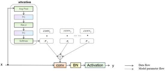
Figure 1.
Dynamic convolutional structure.
This design enables the network to focus on the most relevant spatial patterns in the data and adapt to signal variations, particularly under strong noise. By dynamically adjusting the kernel responses, the model enhances its ability to capture subtle and diverse fault-related features that static convolutions may overlook.
2.3. Selective Kernel Attention
Selective Kernel Attention is an attention mechanism that extracts multi-scale features by introducing convolutional kernels of different sizes and combines it with an attention mechanism to select important convolutional features. The structure of SKAttention, is shown in Figure 2, which consists of 3 parts, namely Split, Fuse, and Select. In the Split part, 3 × 3 and 5 × 5 convolution operations are performed on the input image respectively to obtain feature maps and 2 feature maps. Fuse is the part that calculates the weights of the 2 convolution kernels by summing their. The feature maps of the two are summed up by elements, and then averaged along the H and W dimensions, to obtain a one-dimensional vector with C × 1 × 1. The weight information indicates the importance of the information of the individual channels.
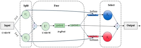
Figure 2.
Structure of Selective Kernel Attention.
Where U is the channel statistical information generated by global average pooling (AvgPool). Then a linear transformation is used to map the original C-dimensional information into Z-dimensional information, and then 2 linear transformations are used respectively to change from the Z-dimension to the original C-dimension, which completes the extraction of the information channel dimensions. The Select part is normalized by the Softmax function, and the corresponding weight scores of each Channel are computed, the weights are applied to the feature maps, and finally, the 2 new feature maps are fused to get the final output image. The output image is compared with the input image, after the information channel is refined, more key information is fused, and the key information of the image is enhanced.
This mechanism improves the model’s ability to suppress noise and focus on fault-relevant patterns, thereby enhancing diagnostic precision in complex environments.
2.4. Enhanced DRSN
The Deep Residual Shrinkage Network (DRSN) is composed of multiple Residual Shrinkage Building Units (RSBUs) stacked sequentially. Each RSBU extends the traditional residual block by incorporating a soft thresholding function and an attention mechanism, enabling the network to suppress redundant information and enhance meaningful features under strong noise conditions. This significantly improves the model’s robustness and feature representation capability.
However, the convolution operations in the original RSBUs are based on fixed kernels, which limits their adaptability to the non-stationary nature of vibration signals in noisy environments. This restricts the model’s generalization and diagnostic performance in real industrial scenarios. Fixed receptive fields in standard convolutions may amplify high-frequency noise or mask critical low-frequency fault features, making it difficult to extract useful diagnostic information.
To address this challenge, the proposed method integrates a Dynamic Convolution mechanism and redesigns the RSBU structure. First, the one-dimensional vibration signals are transformed into two-dimensional time frequency images using Continuous Wavelet Transform (CWT), which helps the model capture localized time frequency features more effectively. Since the original RSBU was designed for 1D sequences and cannot be directly applied to 2D inputs, all 1D convolution operations are replaced with 2D dynamic convolutions, resulting in the enhanced residual block named Dynamic-2D RSBU (DRSBU), as illustrated in Figure 3.
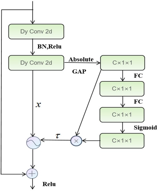
Figure 3.
Structure of DRSBU.
Each DRSBU contains two 3 × 3 2D dynamic convolution layers, followed by batch normalization, ReLU activation, and a soft thresholding module. After the feature stream passes through the shrinkage module and residual connection, it is activated by ReLU and fed to the next layer. The use of ReLU not only enhances non-linear representation but also improves training speed and convergence efficiency.
The soft thresholding function plays a crucial role in signal denoising by applying a nonlinear transformation to suppress low-amplitude noise. Specifically, it sets values below a learnable threshold to zero and shrinks larger values, thereby retaining essential features while eliminating irrelevant components. The mathematical expression corresponds to typology (5).
where x denotes the input features, y is the output features, and τ is a positive learnable threshold parameter. The function has a good sparsification ability, which helps to improve the robustness of feature expression, and is especially suitable for the task of fault feature extraction in strong noise environments.
2.5. DDRSN-SKA Based Fault Diagnosis
In real-world applications, rolling bearings often operate under strong noise conditions. These environments can cause non-stationary behavior in vibration signals and obscure fault features, making accurate fault diagnosis highly challenging. Traditional deep learning models typically struggle under such conditions due to weak feature extraction and limited anti-interference capabilities, which reduce their ability to reliably identify fault types.
To address these issues, this paper proposes a fault diagnosis method based on the DDRSN-SKA architecture, as illustrated in Figure 4. The method adopts the Deep Residual Shrinkage Network (DRSN) as the backbone and introduces DynamicConv2D to replace traditional static convolution within the RSBU modules. This dynamic convolution mechanism adaptively adjusts the convolutional kernels by weighting multiple learnable filters based on input features, improving the network’s capacity to extract meaningful features.
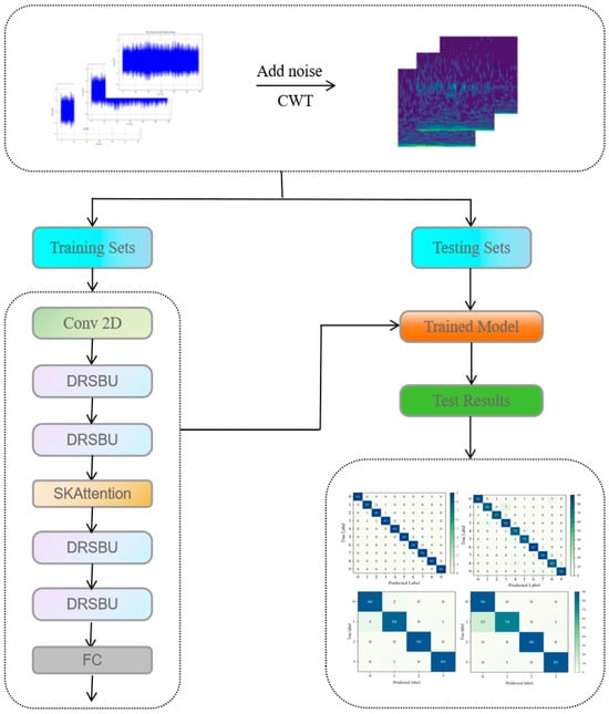
Figure 4.
Framework of DDRSN-SKA fault diagnosis methodology.
Additionally, an SKAttention module is embedded in the intermediate layers of the network. By using multiple convolution kernels of varying sizes and channel-wise attention weights derived via a Softmax function, this module enhances the model’s sensitivity to critical features while suppressing irrelevant information.
Finally, the output features are passed through a fully connected layer to produce class probabilities for different fault types. This architecture allows the model to effectively address the challenges of feature extraction under strong noise and enhances fault classification accuracy.
The specific training and testing process is as follows:
Step 1: Collect original time-domain vibration signals and divide them into training and testing sets according to a predefined ratio.
Step 2: Add Gaussian and Laplace noise with varying signal-to-noise ratios to simulate real-world interference. Apply Continuous Wavelet Transform (CWT) to the noisy signals to generate time frequency representations.
Step 3: Train the DDRSN-SKA model using the training set in batches until convergence.
Step 4: Test the trained model using the test set and evaluate performance metrics to assess diagnostic accuracy.
3. Analysis of Experiments Results
This chapter focuses on analyzing the experimental results of the DDRSN-SKA model to validate its effectiveness in bearing fault diagnosis under strong noise conditions. The analysis will proceeds from the foundational setup to specific performance evaluations. First, Section 3.1 outlines the experimental environment, including the hardware configurations, software frameworks, and key hyperparameter settings, which form the basis for ensuring the reproducibility and reliability of the subsequent experiments. Following this, comparative tests on public and laboratory datasets, ablation studies, and visualizations of results will be presented to comprehensively demonstrate the model’s superiority in noise robustness and diagnostic accuracy.
3.1. Experimental Environment and Parameter Settings
In the experiments, all the programs in this paper were run on a computer with an Inter CORE i7-10750H processor, and a NVIDIA GeForce RTX 2060 GPU(manufactured by NVIDIA Corporation, Santa Clara, California, USA) graphics card, implemented with Python 3.9 as the programming language and the PyTorch 1.13 deep learning framework. In the training phase, the learning rate lr is set to 0.001, the Batch size is 64, and the optimization algorithm is Adam, which has the characteristics of fast computational efficiency and small memory requirement to accelerate the convergence of the model.
The model structure parameters are set as shown in Table 1, where the second column represents the output dimensions of the different layers in the format of channels width height.

Table 1.
Relevant parameters of the model architecture of this paper.
3.2. Case 1: CWRU Bearing Dataset
3.2.1. Dataset Description
The Case Western Reserve University (CWRU) open bearing dataset is the most commonly used dataset in the field of fault diagnosis to verify the validity of diagnostic algorithms. The CWRU bearing experimental bench consists of a 2 hp motor, a dynamometer, and torque transducers, as shown in Figure 5. The sampling frequency of the dataset is 12 kHz and 48 kHZ, the test bearing model of the test bearing is SKF6205-2RSJEM, and single points of failure is set up by EDM technology, and the types of defects of the bearing are rolling body damage, outer ring damage, and inner ring damage, and each defect type contains three kinds of damage diameters: 0.1778 mm, 0.3556 mm, and 0.5334 mm, In this paper, the sampling frequency of 12 kHz is selected is as the sampling frequency of the test bearing, and the sampling frequency of 12 kHz is selected as the sampling frequency of the test bearing. The vibration signal data of the rolling bearing at the DE end, with a sampling frequency of 12 kHZ and a rotational speed of 1730 r/min, is selected, which contains 10 different states. Rolling body faults with fault diameters of 0.1778 mm, 0.3556 mm, and 0.5334 mm (labeled BA_1, BA_2, and BA_3, respectively), inner ring faults with fault diameters of 0.1778 mm, 0.3556 mm, and 0.5334 mm (labeled IR_1, IR_2, and IR_3, respectively), and rolling bearing faults with fault diameters of 0.1778 mm, 0.3556 mm, and 0.5334 mm outer ring faults (labeled OR_1, OR_2, and OR_3, respectively).
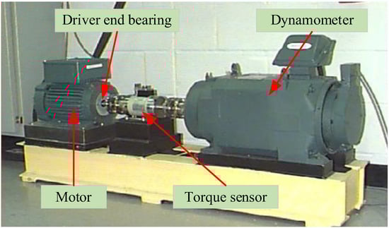
Figure 5.
CWRU bearing test stand.
Randomly intercept 300 samples from each of the 10 bearing statedata, there are 10 kinds of states, and a total of 3000 samples are obtained, and the length of each sample is 2048 sampling points. The ratio of the training set and validation set are divided according to the ratio of 7:3, and 2100 training samples and 900 validation samples are obtained. The information of the Experiment 1 dataset is shown in Table 2.
Table 2.
Test one bearing data set.
In order to study the influence of noise signals on the diagnostic effect of the model, Gaussian noise with different signal-to-noise ratios is firstly added to the original vibration signals, and then the continuous wavelet transform is performed on the noise-containing vibration signals to generate two-dimensional colorful wavelet time frequency maps, and at the same time, in order to avoid the influence on the classification results, the legend and coordinate system are set not to be displayed, and finally, the mesh-normalized compression is carried out on the pictures to generate a 128 × 128 × 3 pixel format.
Figure 6 shows the wavelet time frequency plots for each health state of the bearing when the signal-to-noise ratio of −8 is added. From Figure 6, it can be seen that there is a large amount of noise in the images, which is randomly and irregularly distributed in dots and diffusion, leading to confusion and blurring of local features of the images, masking the true characteristics of the fault signals and making it difficult to accurately recognize the fault modes.
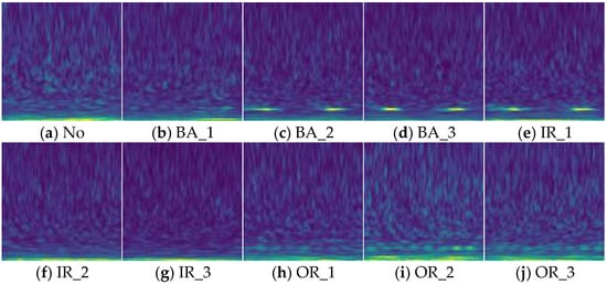
Figure 6.
Wavelet time frequency plots for 10 health states at SNR of −8.
3.2.2. Comparative Experiments
To evaluate the impact of strong noise on bearing fault diagnosis, Gaussian and Laplace noise with varying signal-to-noise ratios (SNRs) were added to the original vibration signals to simulate real-world noisy conditions.
To assess the effectiveness of the proposed model, comparative experiments were conducted with several deep learning baselines, including ResNet, DRSN-CS, DRSN-Transformer, and 1DProposed. Table 3 and Table 4 summarize the diagnostic accuracies of each model under different noise levels.
Table 3.
Diagnostic accuracy of each model under Gaussian noise with different signal-to-noise ratios.
Table 4.
Diagnostic accuracy of each model under Laplace noise with different signal-to-noise ratios.
As shown in Table 3 and Table 4, when clean signals are used as input, all models achieved comparable performance with high diagnostic accuracy. However, as the noise level increases, the performance of the baseline models degrades significantly, highlighting their limited robustness to noise interference. In contrast, the proposed DDRSN-SKA model consistently demonstrates superior performance and maintains high accuracy across all SNR levels.
Specifically, at an SNR of −8 dB, the DDRSN-SKA model improves diagnostic accuracy by 3.63% over DRSN-Transformer and by 2.42% over the 1DProposed model, which does not utilize CWT. These results underscore the effectiveness of time frequency representations in enhancing noise robustness. Across all noise intensities, the proposed model achieves the highest accuracy, confirming its strong anti-noise capability.
To further evaluate classification accuracy and feature separability, confusion matrices and t-SNE visualizations were employed. Figure 7 and Figure 8 illustrate the confusion matrices and t-SNE plots for the DDRSN-SKA model under Gaussian and Laplace noise conditions, respectively. The confusion matrix provides a clear depiction of true versus predicted labels, with diagonal entries representing correctly classified samples. The t-SNE plots utilize color-coded markers to distinguish categories, allowing for intuitive interpretation of feature clustering under noisy conditions.
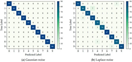
Figure 7.
Confusion matrix of this paper’s model in a SNR = −8 dB noise environment.
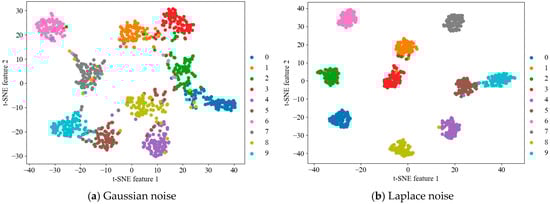
Figure 8.
Viewable view of the model of this paper in a SNR = −8 dB noise environment.
Figure 7a is a 10 × 10 confusion matrix under Gaussian noise (labels 0–9), corresponding to ten bearing states (see Table 2). The vertical axis denotes true labels and the horizontal axis predicted labels, with main diagonal values representing correctly classified faults and non-diagonal values indicating misclassifications. Figure 7b, the confusion matrix under Laplace noise, retains the same structure and axis definitions as Figure 7a for direct performance comparison. Under Gaussian noise, the model stably identifies most fault types (e.g., categories 0, 1, 4, 6, 7) with minimal sporadic misclassifications, reflecting fine discriminative ability; in contrast, Laplace noise causes more obvious interference, especially in categories 1, 2, 4, 5, indicating overlapping feature.
Figure 8a is a t-SNE plot under Gaussian noise, where each colored point (matching the legend) represents a fault sample, showing the spatial distribution of projected high-dimensional features. Fault features form clear, well-separated clusters here, validating the model’s effective feature learning and discrimination even at −8 dB, while complementing the confusion matrix’s quantitative accuracy. Figure 8b, the t-SNE plot under Laplace noise, uses the same color coding and sample rules for comparison; some categories overlap here, consistent with the confusion matrix’s 91.77% accuracy (vs. 98.44% under Gaussian noise). Despite this, most categories remain separable, highlighting the model’s robust feature extraction in adverse noise.
Remarkably, at a high SNR of 4 dB, the proposed model achieves near-perfect classification across all fault categories, demonstrating its effectiveness in low-noise environments. Even under severe noise (SNR = −8 dB), the model attains diagnostic accuracies of 98.44% for Gaussian noise and 91.77% for Laplace noise. These results affirm the DDRSN-SKA model’s exceptional robustness and strong generalization performance in complex noise conditions, positioning it as a leading solution in noise-resilient bearing fault diagnosis.
3.2.3. Ablation Experiments
To evaluate the contribution of individual components within the proposed model, ablation experiments were conducted by selectively removing the Dynamic Convolution and SKAttention modules. These tests were performed under strong noise conditions by adding Gaussian and Laplace noise at an SNR of −8 dB to the input signals. The classification accuracies of the model under four different configurations are reported in Table 5.
Table 5.
Diagnostic accuracy of ablation experimental models (%).
The configurations are defined as follows:
Only Dynamic Convolution: The SKAttention module is removed while retaining Dynamic Convolution.
Only SKAttention: The Dynamic Convolution layers are replaced with standard convolution layers while keeping SKAttention.
Neither: Both the Dynamic Convolution layers are replaced with standard convolution and the SKAttention module is removed.
Both: The complete proposed model, incorporating both Dynamic Convolution and SKAttention.
Results from Table 4 reveal that both modules contributed significantly to the model’s performance. Under Gaussian noise, the full model (“Both”) achieved an accuracy of 98.44%, surpassing the configurations with only Dynamic Convolution (97.11%) and only SKAttention (97.44%). Similarly, under Laplace noise, the full model achieved 91.77%, while the models with only Dynamic Convolution and only SKAttention reached 89.88% and 90.88%, respectively.
These findings demonstrate that Dynamic Convolution and SKAttention each enhance the model’s robustness against noise, and their combination produces a synergistic effect. Specifically, Dynamic Convolution enhances noise tolerance by capturing rich frequency-domain features through multi-scale operations. Meanwhile, SKAttention adaptively emphasizes critical channels and suppresses irrelevant noise by assigning attention weights across feature maps. Together, they significantly improve the model’s ability to extract relevant features in noisy conditions.
In conclusion, the integration of Dynamic Convolution and SKAttention modules is vital for the model’s strong noise resilience and high diagnostic precision in complex fault diagnosis scenarios.
3.3. Case 2: Laboratory Bearing Dataset
3.3.1. Introduction to the Datasets
To further validate the model’s performance, Experiment 2 was conducted using a bearing test bench located in the university’s laboratory, as shown in Figure 9. The test utilized 6007ZM deep groove ball bearings, with fault types including inner ring fault (IF), ball fault (BF), outer ring fault (OF), and a normal state (NF).
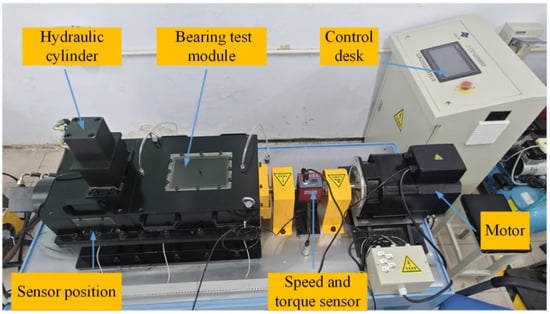
Figure 9.
Laboratory bearing test bench.
During the experiment, the motor speed was set to 1600 rpm, and vibration signals were collected under a radial load of 1500 N. The sampling frequency was configured at 20 kHz. A total of 1200 samples were collected for each fault category, with 840 samples used for training and 360 for testing. Each sample contained 2048 data points. The dataset details are summarized in Table 6.
Table 6.
Experiment 2 bearing data set.
To simulate noisy conditions, Gaussian noise with varying signal-to-noise ratios was added to the original vibration signals. These signals were then transformed using continuous wavelet transform (CWT) to produce two-dimensional wavelet time frequency representations. Examples of these representations at an SNR of −8 dB for each fault type are shown in Figure 10. The presence of significant noise in these images obscures some key fault features, demonstrating the challenge of accurate diagnosis under severe noise interference.
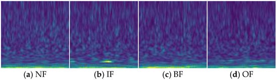
Figure 10.
Wavelet time frequency plots for four health states when SNR is −8.
3.3.2. Comparative Tests
Gaussian and Laplace noise with varying intensities were added to the bearing vibration dataset collected in the laboratory. The experimental results are presented in Table 7 and Table 8. As the signal-to-noise ratio (SNR) decreases, the diagnostic accuracy of all models declines accordingly. However, the proposed DDRSN-SKA model consistently achieves the highest accuracy across all noise levels.
Table 7.
Diagnostic accuracy (Gaussian noise) for each model with different signal-to-noise ratios.
Table 8.
Diagnostic accuracy of different models with different signal-to-noise ratios (Laplace noise).
Notably, under extreme noise conditions (SNR = −8 dB), the proposed model achieves diagnostic accuracies of 97.50% and 94.44% under Gaussian and Laplace noise, respectively. These results surpass those of other models, including the state-of-the-art DRSN-Transformer, by 2.23% and 1.17%, respectively, clearly demonstrating the superior robustness and effectiveness of the proposed approach.
Figure 11 illustrates the classification performance of each model under Gaussian noise with SNR = −8 dB. It can be observed that all models primarily misclassify inner ring faults as normal conditions. This suggests that inner ring fault features are relatively weak and closely resemble the vibration signatures of normal bearings, increasing the likelihood of misclassification.
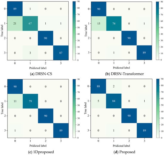
Figure 11.
Confusion matrices of different models under Gaussian noise.
Among the models compared, the proposed method exhibits the fewest misclassifications for ball faults, with only 6 out of 90 samples incorrectly identified. This further confirms that the DDRSN-SKA model outperforms other approaches in recognizing different fault types under strong noise interference, reinforcing the validity and superiority of the proposed method.
4. Conclusions
In conclusion, this study addresses the key scientific questions by demonstrating that the proposed DDRSN-SKA model effectively extracts fault features from rolling bearing signals severely obscured by strong Gaussian and Laplace noise, validates the enhanced anti-noise capability through the fusion of dynamic convolution and SKAttention, and proves its superior diagnostic accuracy over existing methods under varying noise conditions.
The overall added value of this research lies in both theoretical and practical aspects. Theoretically, it introduces a novel framework combining dynamic feature extraction and attention-driven optimization into deep residual shrinkage networks, offering new insights for noise-robust fault diagnosis. Practically, the model’s high accuracy (98.44% under Gaussian noise and 94.44% under Laplace noise at SNR = −8 dB) on both the CWRU and laboratory datasets provides a reliable solution for industrial applications, potentially reducing unplanned downtime and maintenance costs in manufacturing.
The proposed model is designed for rolling bearing fault diagnosis under strong noise conditions and demonstrates robust capability in extracting critical fault features. However, in real industrial scenarios, bearing signals are often affected by nonlinear characteristics, multi-sensor interactions, and complex noise types, and the model’s adaptability under extreme noise and variable operating conditions remains limited. Future research will focus on the integration of multi-task learning and lightweight deployment: by constructing a unified framework that combines fault classification, remaining useful life prediction, and health assessment, task interdependencies can be fully leveraged to improve diagnostic comprehensiveness; meanwhile, techniques such as knowledge distillation, model pruning, and quantization can optimize network structure and computational efficiency, enabling efficient deployment on low-power edge devices and further enhancing the model’s robustness and practical applicability in complex industrial environments.
Author Contributions
Conceptualization, X.L. and J.W. (Jixuan Wang); data curation, X.L., J.W. (Jiahao Wang) and J.W. (Jianqiang Wang); formal analysis, J.L.; validation, J.C., J.W. (Jianqiang Wang) and X.Y.; writing—original draft preparation, J.W. (Jixuan Wang); writing—review and editing, X.L. and J.W. (Jiahao Wang); visualization, J.C.; supervision, X.L.; project administration, X.L. All authors have read and agreed to the published version of the manuscript.
Funding
This work was supported by the Department of Education of Jilin Province under grant JJKH20251092CY, Changchun University, under grant ZKP202018, and Changchun Jiamei Machinery Manufacturing Co., Ltd., under grant 2024JBH01LX6.
Data Availability Statement
The data used in this study are derived from both open-source datasets and private datasets, respectively.
Conflicts of Interest
The authors declare no conflicts of interest.
References
- Lee, J.; Wu, F.; Zhao, W.; Ghaffari, M.; Liao, L.; Siegel, D. Prognostics and health management design for rotary machinery systems—Reviews, methodology and applications. Mech. Syst. Signal Process. 2014, 42, 314–334. [Google Scholar] [CrossRef]
- Rai, A.; Upadhyay, S.H. A review on signal processing techniques utilized in the fault diagnosis of rolling element bearings. Tribol. Int. 2016, 96, 289–306. [Google Scholar] [CrossRef]
- Zhang, T.; Chen, J.; Li, F.; Zhang, K.; Lv, H.; He, S.; Xu, E. Intelligent fault diagnosis of machines with small & imbalanced data: A state-of-the-art review and possible extensions. ISA Trans. 2022, 119, 152–171. [Google Scholar] [CrossRef] [PubMed]
- Xu, Y.; Zhang, K.; Ma, C.; Li, X.; Zhang, J. An Improved Empirical Wavelet Transform and Its Applications in Rolling Bearing Fault Diagnosis. Appl. Sci. 2018, 8, 2352. [Google Scholar] [CrossRef]
- Zhou, J.; Qin, Y.; Kou, L.; Yuwono, M.; Su, S. Fault detection of rolling bearing based on FFT and classification. J. Adv. Mech. Des. Syst. Manuf. 2015, 9, JAMDSM0056. [Google Scholar] [CrossRef]
- Tse, P.W.; Peng, Y.H.; Yam, R. Wavelet Analysis and Envelope Detection For Rolling Element Bearing Fault Diagnosis—Their Effectiveness and Flexibilities. J. Vib. Acoust. 2001, 123, 303–310. [Google Scholar] [CrossRef]
- Suthaharan, S. Support Vector Machine. In Machine Learning Models and Algorithms for Big Data Classification; Springer: Boston, MA, USA, 2016; Volume 36, pp. 207–235. [Google Scholar] [CrossRef]
- Hamadache, M.; Lee, D. Principal component analysis based signal-to-noise ratio improvement for inchoate faulty signals: Application to ball bearing fault detection. Int. J. Control Autom. Syst. 2017, 15, 506–517. [Google Scholar] [CrossRef]
- Xie, F.; Li, G.; Song, C.; Song, M. The Early Diagnosis of Rolling Bearings’ Faults Using Fractional Fourier Transform Information Fusion and a Lightweight Neural Network. Fractal Fract. 2023, 7, 875. [Google Scholar] [CrossRef]
- Shen, W.; Xiao, M.; Wang, Z.; Song, X. Rolling Bearing Fault Diagnosis Based on Support Vector Machine Optimized by Improved Grey Wolf Algorithm. Sensors 2023, 23, 6645. [Google Scholar] [CrossRef]
- Zhang, S.; Zhang, S.; Wang, B.; Habetler, T.G. Deep Learning Algorithms for Bearing Fault Diagnostics—A Comprehensive Review. IEEE Access 2020, 8, 29857–29881. [Google Scholar] [CrossRef]
- Zhao, R.; Yan, R.; Chen, Z.; Mao, K.; Wang, P.; Gao, R.X. Deep learning and its applications to machine health monitoring. Mech. Syst. Signal Process. 2019, 115, 213–237. [Google Scholar] [CrossRef]
- Chua, L.O.; Roska, T. The CNN paradigm. IEEE Trans. Circuits Syst. Fundam. Theory Appl. 1993, 40, 147–156. [Google Scholar] [CrossRef]
- Alzubaidi, L.; Zhang, J.; Humaidi, A.J.; Al-Dujaili, A.; Duan, Y.; Al-Shamma, O.; Santamaría, J.; Fadhel, M.A.; Al-Amidie, M.; Farhan, L. Review of deep learning: Concepts, CNN architectures, challenges, applications, future directions. J. Big Data 2021, 8, 53. [Google Scholar] [CrossRef] [PubMed]
- Wang, Z.; Xu, X.; Song, D.; Zheng, Z.; Li, W. A Novel Bearing Fault Diagnosis Method Based on Improved Convolutional Neural Network and Multi-Sensor Fusion. Machines 2025, 13, 216. [Google Scholar] [CrossRef]
- Xu, T.; Lv, H.; Lin, S.; Tan, H.; Zhang, Q. A fault diagnosis method based on improved parallel convolutional neural network for rolling bearing. Proc. Inst. Mech. Eng. Part G J. Aerosp. Eng. 2023, 237, 2759–2771. [Google Scholar] [CrossRef]
- Li, S.; Ji, J.C.; Xu, Y.; Sun, X.; Feng, K.; Sun, B.; Wang, Y.; Gu, F.; Zhang, K.; Ni, Q. IFD-MDCN: Multibranch denoising convolutional networks with improved flow direction strategy for intelligent fault diagnosis of rolling bearings under noisy conditions. Reliab. Eng. Syst. Saf. 2023, 237, 109387. [Google Scholar] [CrossRef]
- Khawaja, A.U.; Shaf, A.; Thobiani, F.A.; Ali, T.; Irfan, M.; Pirzada, A.R.; Shahkeel, U. Optimizing Bearing Fault Detection: CNN-LSTM with Attentive TabNet for Electric Motor Systems. Comput. Model. Eng. Sci. 2024, 141, 2399–2420. [Google Scholar] [CrossRef]
- Zhang, W.-T.; Liu, L.; Cui, D.; Ma, Y.-Y.; Huang, J. An Anti-Noise Convolutional Neural Network for Bearing Fault Diagnosis Based on Multi-Channel Data. Sensors 2023, 23, 6654. [Google Scholar] [CrossRef]
- Dong, Z.; Zhao, D.; Cui, L. An intelligent bearing fault diagnosis framework: One-dimensional improved self-attention-enhanced CNN and empirical wavelet transform. Nonlinear Dyn. 2024, 112, 6439–6459. [Google Scholar] [CrossRef]
- Chen, Y.; He, Y.; Li, Z.; Chen, L.; Zhang, C. Remaining useful life prediction and state of health diagnosis of lithium-ion battery based on second-order central difference particle filter. IEEE Access 2020, 8, 37305–37313. [Google Scholar] [CrossRef]
- Chen, Z.; Mauricio, A.; Li, W.; Gryllias, K. A deep learning method for bearing fault diagnosis based on Cyclic Spectral Coherence and Convolutional Neural Networks. Mech. Syst. Signal Process. 2020, 140, 106683. [Google Scholar] [CrossRef]
- Qi, J.; Chen, Z.; Kong, Y.; Qin, W.; Qin, Y. Attention-guided graph isomorphism learning: A multi-task framework for fault diagnosis and remaining useful life prediction. Reliab. Eng. Syst. Saf. 2025, 263, 111209. [Google Scholar] [CrossRef]
- Qi, J.; Chen, Z.; Uhlmann, Y.; Schullerus, G. Sensorless Robust Anomaly Detection of Roller Chain Systems Based on Motor Driver Data and Deep Weighted KNN. IEEE Trans. Instrum. Meas. 2025, 74, 1–13. [Google Scholar] [CrossRef]
- Tong, J.; Tang, S.; Wu, Y.; Pan, H.; Zheng, J. A fault diagnosis method of rolling bearing based on improved deep residual shrinkage networks. Measurement 2023, 206, 112282. [Google Scholar] [CrossRef]
- Li, X.; Chen, J.; Wang, J.; Wang, J.; Li, X.; Kan, Y. Research on Fault Diagnosis Method of Bearings in the Spindle System for CNC Machine Tools Based on DRSN-Transformer. IEEE Access 2024, 12, 74586–74595. [Google Scholar] [CrossRef]
- Li, X.; Wang, J.; Wang, J.; Wang, J.; Chen, J.; Yu, X. Research on CNC Machine Tool Spindle Fault Diagnosis Method Based on DRSN–GCE Model. Algorithms 2025, 18, 304. [Google Scholar] [CrossRef]
- Li, X.; Chen, J.; Wang, J.; Wang, J.; Wang, J.; Li, X.; Kan, Y. Multi-Scale Channel Mixing Convolutional Network and Enhanced Residual Shrinkage Network for Rolling Bearing Fault Diagnosis. Electronics 2025, 14, 855. [Google Scholar] [CrossRef]
- Wang, L.; Zou, T.; Cai, K.; Liu, Y. Rolling bearing fault diagnosis method based on improved residual shrinkage network. J. Braz. Soc. Mech. Sci. Eng. 2024, 46, 172. [Google Scholar] [CrossRef]
- Chen, W.; Sun, K.; Li, X.; Xiao, Y.; Xiang, J.; Mao, H. Adaptive Multi-Channel Residual Shrinkage Networks for the Diagnosis of Multi-Fault Gearbox. Appl. Sci. 2023, 13, 1714. [Google Scholar] [CrossRef]
Disclaimer/Publisher’s Note: The statements, opinions and data contained in all publications are solely those of the individual author(s) and contributor(s) and not of MDPI and/or the editor(s). MDPI and/or the editor(s) disclaim responsibility for any injury to people or property resulting from any ideas, methods, instructions or products referred to in the content. |
© 2025 by the authors. Licensee MDPI, Basel, Switzerland. This article is an open access article distributed under the terms and conditions of the Creative Commons Attribution (CC BY) license (https://creativecommons.org/licenses/by/4.0/).