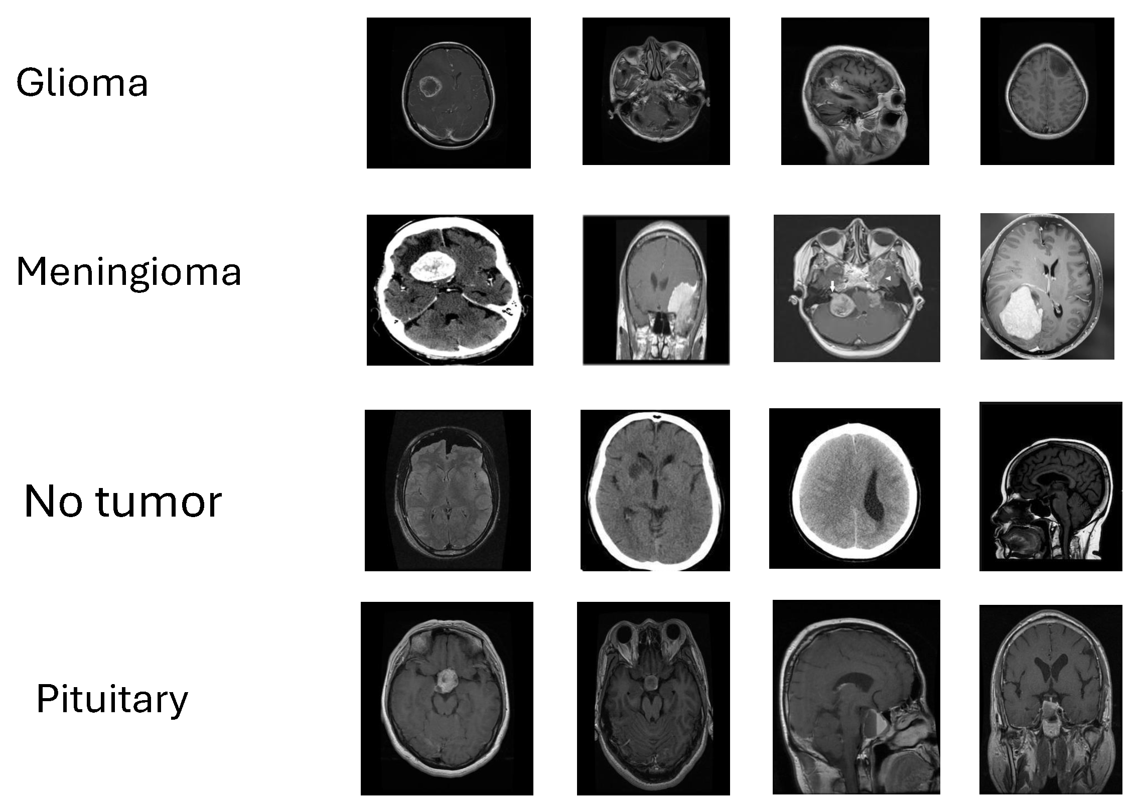
Figure 1.
Representative MRI slices from the four study classes—glioma, meningioma, pituitary tumor, and no tumor—illustrating appearance variability used for validation.
Figure 1.
Representative MRI slices from the four study classes—glioma, meningioma, pituitary tumor, and no tumor—illustrating appearance variability used for validation.
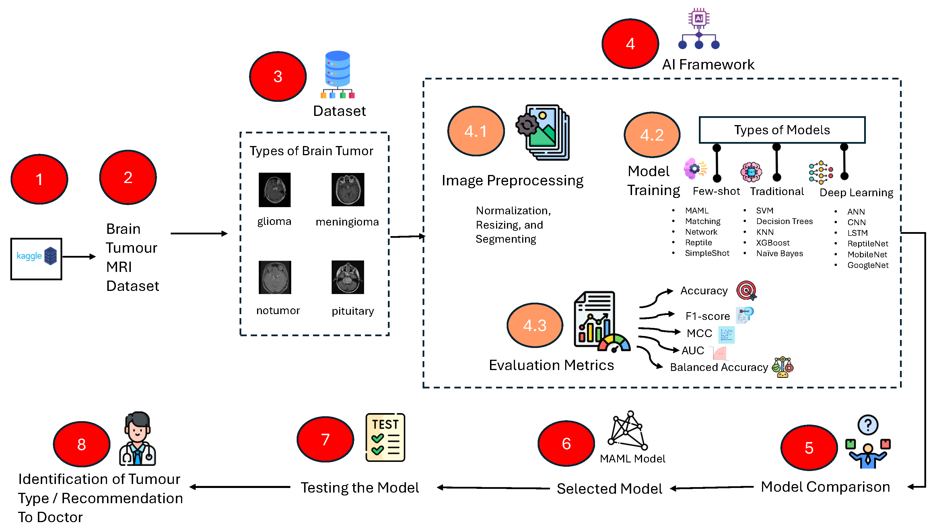
Figure 2.
Stepwise Study workflow: data acquisition (Kaggle), labeling, preprocessing (resize/normalize/augment), model training (traditional ML, deep learning, few-shot learning), evaluation (accuracy, balanced accuracy, F1, MCC, AUC-ROC), model selection, and test-time inference for clinical decision support.
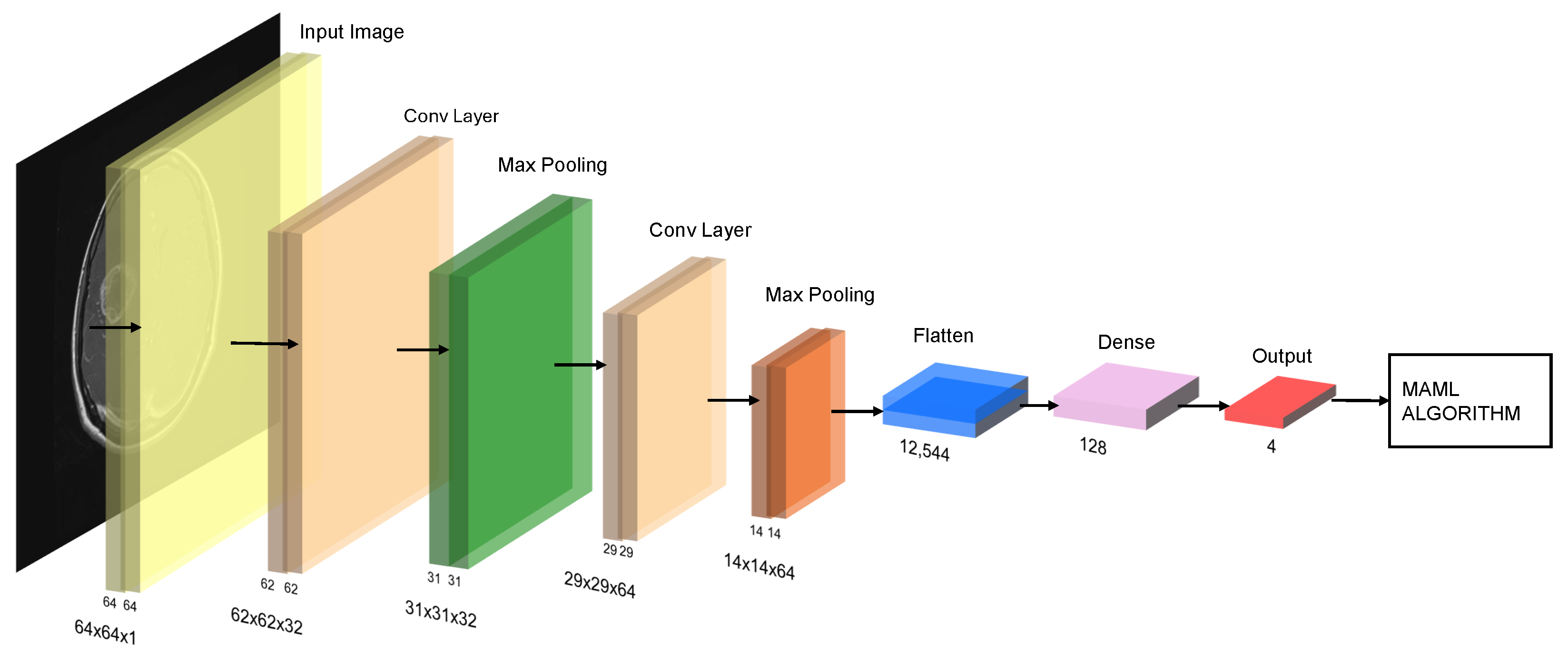
Figure 3.
Schematic of the MAML (Model-Agnostic Meta-Learning) pipeline with a CNN backbone: stacked convolution + pooling blocks, feature flattening, dense layer, and softmax output over four classes.
Figure 3.
Schematic of the MAML (Model-Agnostic Meta-Learning) pipeline with a CNN backbone: stacked convolution + pooling blocks, feature flattening, dense layer, and softmax output over four classes.
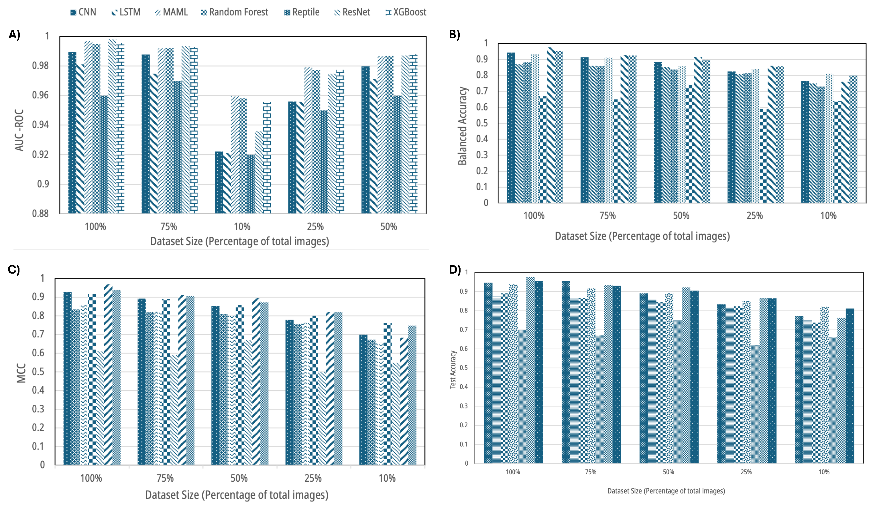
Figure 4.
Aggregate performance across dataset sizes (100%, 75%, 50%, 25%, 10%): (A) AUC-ROC, (B) balanced accuracy, (C) Matthews correlation coefficient (MCC), and (D) test accuracy for traditional ML, deep learning, and few-shot learning models. Error modes and per-class shifts are detailed in later figures.
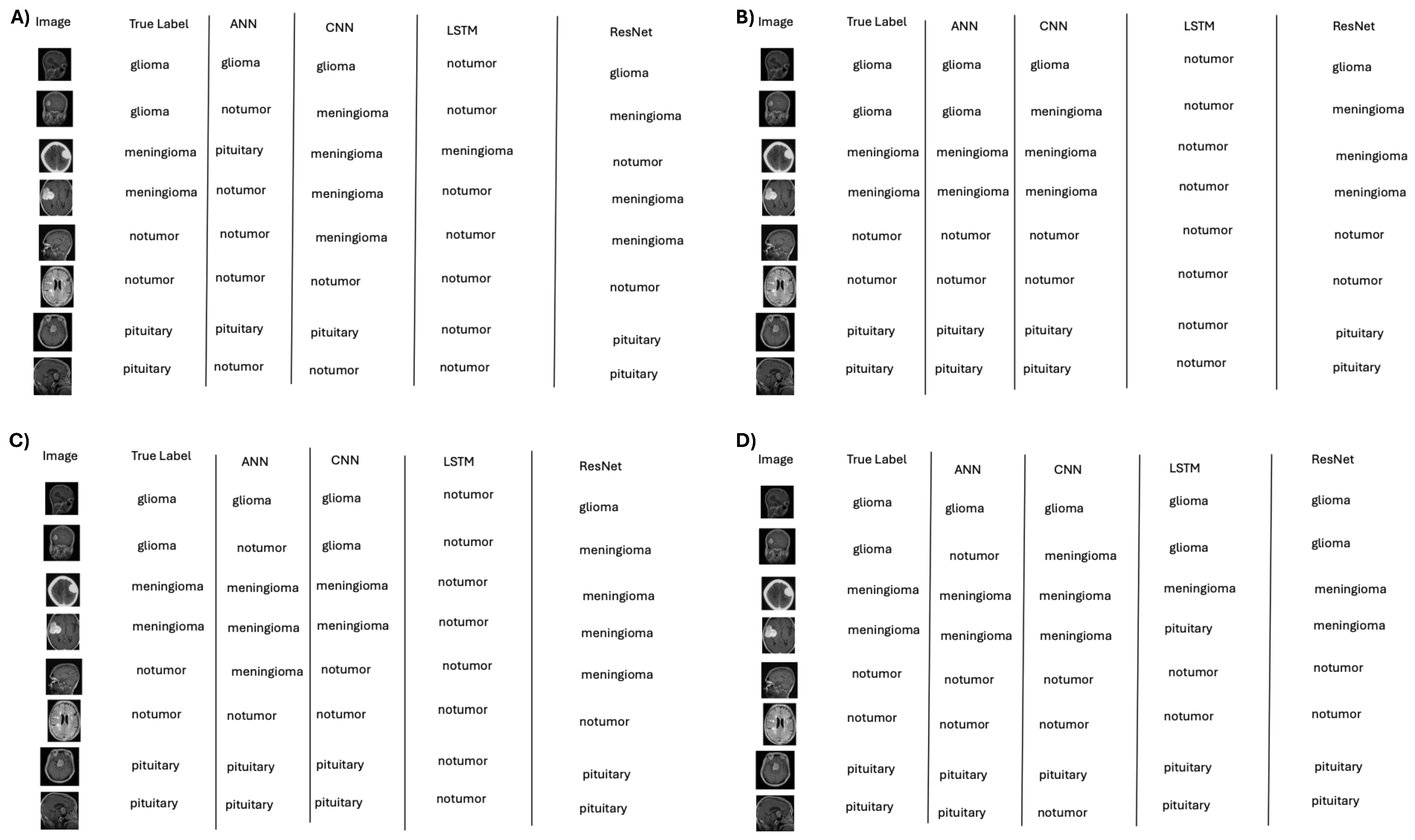
Figure 5.
Representative classifications by deep learning models across data regimes: (A) 10%, (B) 50%, (C) 75%, and (D) 100% training data. Accuracy improves with data scale, with persistent difficulty for “no tumor” in low-data settings.
Figure 5.
Representative classifications by deep learning models across data regimes: (A) 10%, (B) 50%, (C) 75%, and (D) 100% training data. Accuracy improves with data scale, with persistent difficulty for “no tumor” in low-data settings.
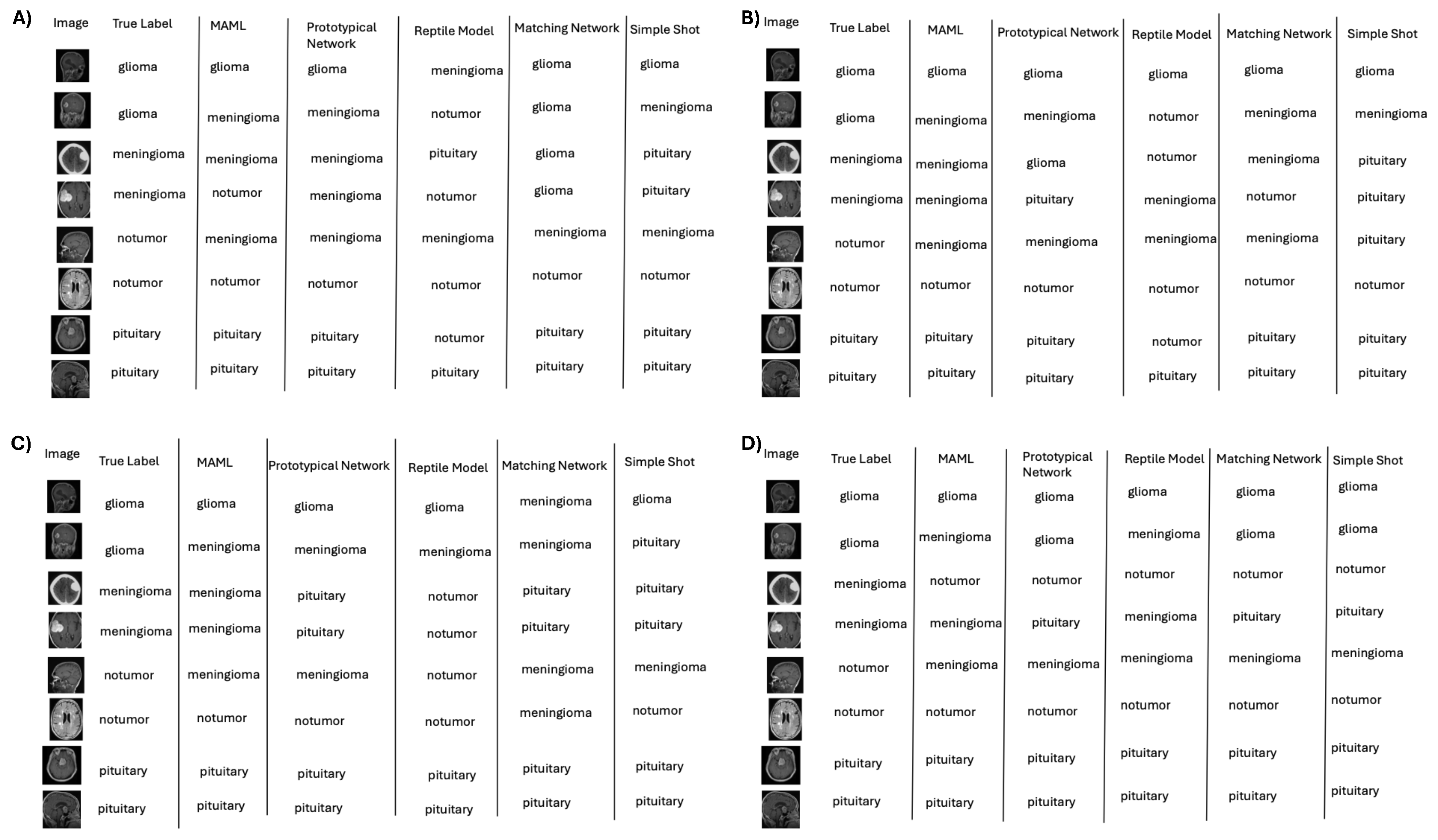
Figure 6.
Representative classifications by few-shot learning (e.g., MAML) across data regimes: (A) 10%, (B) 50%, (C) 75%, and (D) 100%; performance remains competitive under label scarcity.
Figure 6.
Representative classifications by few-shot learning (e.g., MAML) across data regimes: (A) 10%, (B) 50%, (C) 75%, and (D) 100%; performance remains competitive under label scarcity.
Figure 7.
Representative classifications by traditional machine learning models across data regimes: (A) 10%, (B) 50%, (C) 75%, and (D) 100%; SVM and Random Forest improve with more data but show early confusion of “no tumor” with pituitary.
Figure 7.
Representative classifications by traditional machine learning models across data regimes: (A) 10%, (B) 50%, (C) 75%, and (D) 100%; SVM and Random Forest improve with more data but show early confusion of “no tumor” with pituitary.
Figure 8.
Interpretability for deep models: Grad-CAM (CNN, ResNet) and saliency (LSTM) highlight decision-relevant regions. Under the 10% dataset, CNN activations on “no tumor” cases often concentrate near the pituitary, explaining false positives. Warmer colors (red/yellow) denote stronger contributions to the predicted class, while cooler colors (blue) indicate weaker contributions.
Figure 9.
Interpretability for few-shot models: Grad-CAM (MAML-lite) and saliency (MatchingNet, ProtoNet, RelationNet) reveal tumor-focused attention on correct cases and background/pituitary activation on specific errors, clarifying cross-class confusions. Warmer colors (red/yellow) indicate regions with higher contribution to the predicted class, while cooler colors (blue) indicate lower contribution.
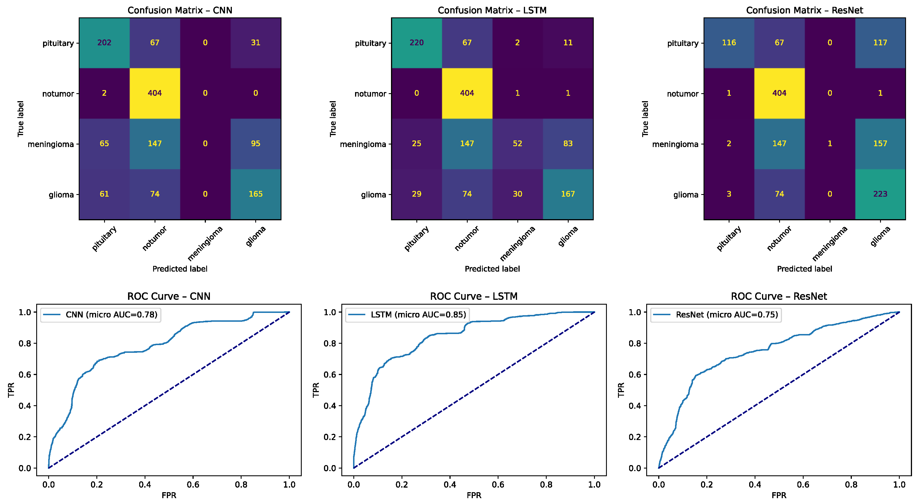
Figure 10.
Confusion matrices for deep learning models: (left) CNN and (right) LSTM on the four-class task. Numbers indicate counts of test samples, with color intensity proportional to frequency (darker = more). Dotted diagonal lines represent perfect classification (all true cases predicted correctly). Common errors include “no tumor” misclassified as pituitary and glioma ↔ meningioma overlap.
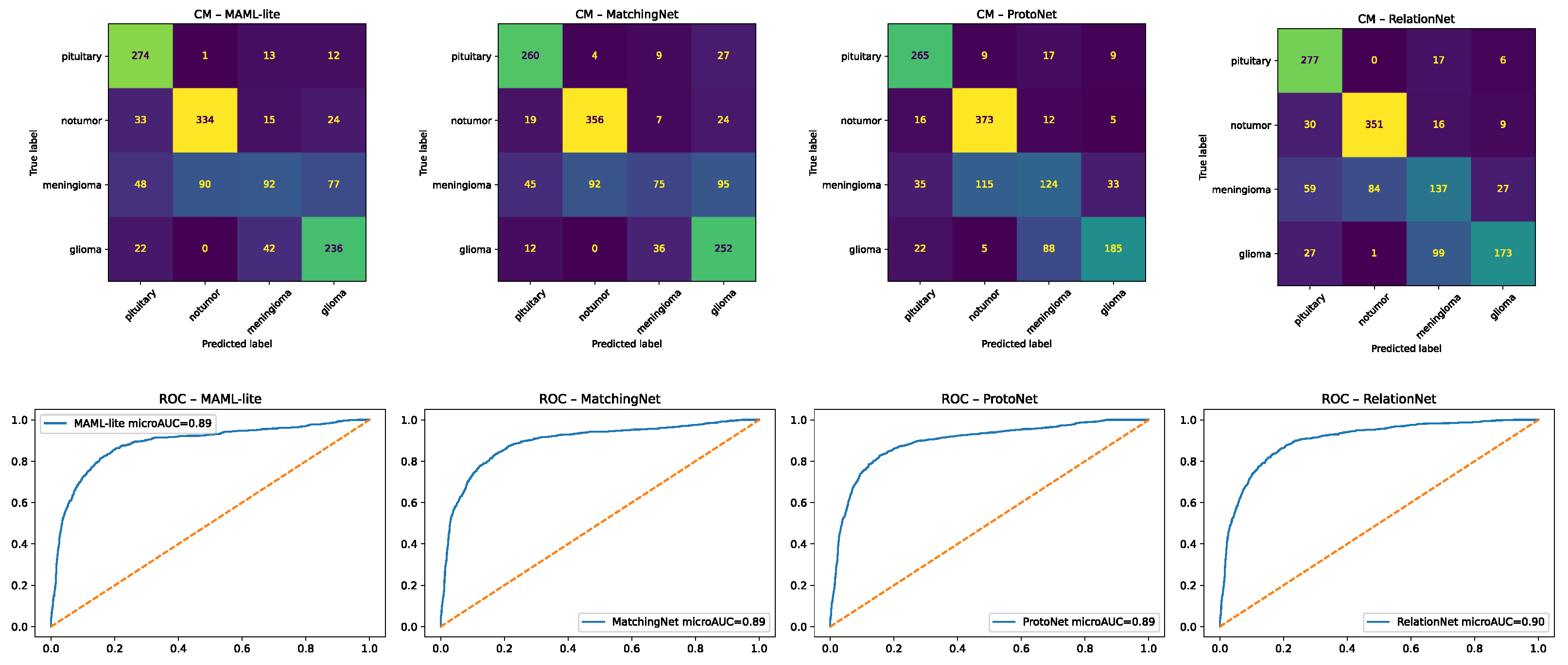
Figure 11.
Confusion matrices for few-shot learning models: (left) MAML-lite and (right) MatchingNet. Numbers show test-sample counts, with color shading scaled to frequency. Dotted diagonal lines mark perfect classification. Few-shot methods improved balance across classes but still show glioma ↔ meningioma confusions in difficult cases.
Figure 12.
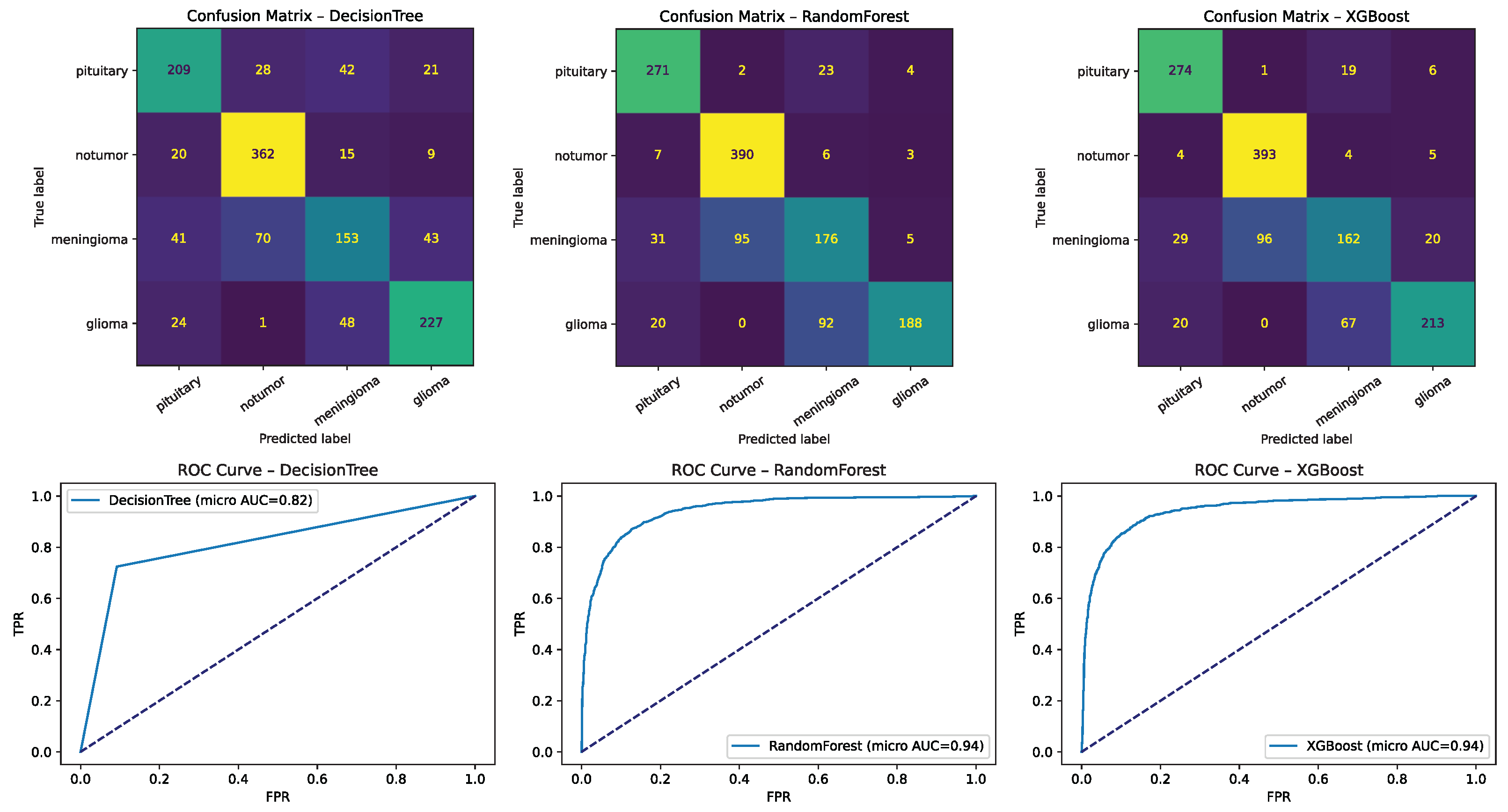
Confusion matrices for representative traditional machine learning models (e.g., SVM/RBF, Random Forest, XGBoost, Logistic Regression). Numbers represent sample counts per cell, with color intensity reflecting frequency. Dotted diagonal lines denote perfect classification. These highlight strengths under ample data and limitations under scarcity, including frequent no tumor ↔ pituitary confusions in low-data settings.
Table 1.
Summary of related work in medical image analysis and few-shot learning: datasets, methods, headline results, contributions, and noted limitations.
Table 1.
Summary of related work in medical image analysis and few-shot learning: datasets, methods, headline results, contributions, and noted limitations.
| Year | Author | Dataset | Method | Results and Contribution | Limitations |
|---|
| 2024 | Alsaleh et al. [3] | 3D Medical | 3D U-Net, MAML | High segmentation accuracy, improving few-shot learning in 3D medical imaging. | Limited availability of labeled data affects training. |
| 2023 | Nayem et al. [6] | Varied Medical | Affinity, Siamese | Achieved excellent performance in prediction tasks using affinity-based approaches. | Initial model configuration limits flexibility. |
| 2020 | Baranwal et al. [7] | REMBRANDT | SVM, CNN | Accuracy: 82.38% (M), 83.01% (G), 95.27% (P). Improved accuracy in brain tumor classification. | Requires a large dataset for effective training. |
| 2020 | Cai et al. [8] | Medical Images | Few-shot, attention | Accuracy: 92.44%. Demonstrated better performance than traditional methods in medical image classification. | Struggles with heterogeneous data. |
| 2020 | Smith et al. [9] | Medical Datasets | Self-supervised | Improved robustness in medical image analysis. Applied successfully in medical imaging tasks. | Limited validation across diverse datasets. |
| 2021 | Jun et al. [10] | MRI Images | Random Forest | Accuracy: 96.3%. Achieved high accuracy in MRI image classification. | Dataset quality and size limitations affect generalizability. |
| 2021 | Mikhael Fasihi [11] | Medical Datasets | LSTM, DWT, DCT | Accuracy: 86.98%. Utilized domain-specific transforms for classification. | High computational complexity. |
| 2021 | Brindha et al. [12] | MRI Images | ANN, CNN | Achieved high detection accuracy, improving detection rates in MRI-based diagnosis. | Requires significant computational resources. |
| 2021 | Seymour et al. [13] | Varied Medical | Meta, few-shot | Effective classification using advanced meta-learning techniques. | Requires careful tuning of hyperparameters. |
| 2022 | Alsubai et al. [14] | Medical Datasets | CNN, LSTM | Demonstrated robust detection by leveraging spatial and temporal features. | High training complexity. |
| 2024 | Gu et al. [15] | Large Datasets | Transfer, MobileNet | Successfully avoided overfitting and enhanced generalization across large datasets. | Dependence on pre-trained models. |
| 2024 | Proposed study | Brain MRI | Few-shot, DL, ML | Achieved 89.00% accuracy, AUC-ROC: 0.9968 for MAML, showcasing potential in brain tumor classification. | Focus is primarily on brain tumors. |
Table 2.
Hyperparameter configurations for traditional machine learning baselines (SVM—linear/polynomial/RBF, Random Forest, Logistic Regression, XGBoost).
Table 2.
Hyperparameter configurations for traditional machine learning baselines (SVM—linear/polynomial/RBF, Random Forest, Logistic Regression, XGBoost).
| Model | Kernel/Type | Additional Configurations |
|---|
| SVM linear kernel | Linear | C = default, gamma = “auto”, probability = True |
| SVM polynomial | Polynomial | degree = 3, C = 1.0, gamma = “scale”, probability = True |
| SVM RBF kernel | RBF | C = 1.0, gamma = “scale”, probability = True |
| Random Forest | - | n_estimators = 100, random_state = 42 |
| Logistic Regression | - | max_iter = 10,000 |
| XGBoost | - | n_estimators = 100, max_depth = 3, random_state = 42 |
Table 3.
Hyperparameter configurations for deep learning models (ANN, CNN, LSTM, ResNet), including optimizer and loss settings.
Table 3.
Hyperparameter configurations for deep learning models (ANN, CNN, LSTM, ResNet), including optimizer and loss settings.
| Model | Kernel/Type | Optimizer | Loss Function | Epochs |
|---|
| ANN | Dense | Adam | sparse_categorical_crossentropy | 10 |
| CNN | Convolutional | Adam | sparse_categorical_crossentropy | 10 |
| LSTM | LSTM | Adam | sparse_categorical_crossentropy | 10 |
| ResNet | Custom | Adam | CrossEntropyLoss | 25 |
Table 4.
Hyperparameter configurations for few-shot and meta-learning models (Prototypical Networks, Matching Networks, SimpleShot, MAML, Reptile).
Table 4.
Hyperparameter configurations for few-shot and meta-learning models (Prototypical Networks, Matching Networks, SimpleShot, MAML, Reptile).
| Model | Type | Optimizer | Loss Function | Epochs |
|---|
| Prototypical Networks | Few-shot | Adam | Cross-entropy loss | 100 |
| Matching Networks | Few-shot | Adam | -ve log-likelihood loss | 100 |
| SimpleShot | Few-shot | N/A | N/A | N/A |
| MAML | Meta-learning | SGD, Adam | Sparse categorical cross-entropy | 10 |
| Reptile | Meta-learning | Adam | Sparse categorical cross-entropy | 10 |
Table 5.
Additional architectural details for all models (e.g., layer stacks, prototype computation, similarity metrics, meta-learning updates) used to ensure reproducibility.
Table 5.
Additional architectural details for all models (e.g., layer stacks, prototype computation, similarity metrics, meta-learning updates) used to ensure reproducibility.
| Model | Additional Configurations |
|---|
| ANN | Layers: flatten, dense (128, ReLU), dense (4, softmax) |
| CNN | Layers: Conv2D, MaxPooling2D, flatten, dense, activation (ReLU/softmax) |
| LSTM | Input shape: (1, features), Layers: LSTM (128), dense (128, ReLU) |
| ResNet | Custom blocks, adaptive average pooling, modified fc layer for 4 classes |
| Prototypical Networks | Prototypes computed as mean of support features |
| Matching Networks | LSTM-based feature encoding, softmax over similarities |
| SimpleShot | Cosine similarity, feature normalization |
| MAML | Meta-learning with rapid adaptation |
| Reptile | Gradient updates with full dataset adaptation |
Table 6.
Confusion matrix definition.
Table 6.
Confusion matrix definition.
| | Predicted Positive | Predicted Negative |
|---|
| Actual Positive | True positive | FN |
| Actual Negative | FP | TN |
Table 7.
Computational complexity of all models—trainable parameters and floating-point operations (FLOPs) per inference/episode—supporting deployment feasibility analyses.
Table 7.
Computational complexity of all models—trainable parameters and floating-point operations (FLOPs) per inference/episode—supporting deployment feasibility analyses.
| Model | Trainable Parameters | FLOPs (per Inference/Episode) |
|---|
| CNN | ∼2.3 M | 1.8 GFLOPs |
| LSTM | ∼3.1 M | 2.2 GFLOPs |
| ResNet | ∼11.2 M | 4.5 GFLOPs |
| MAML-lite | ∼2.6 M | 2.0 GFLOPs |
| MatchingNet | ∼2.9 M | 2.1 GFLOPs |
| ProtoNet | ∼2.5 M | 1.9 GFLOPs |
Table 8.
Class distribution in the Kaggle Brain Tumor MRI Dataset (n = 7023): glioma, meningioma, pituitary tumor, and no tumor; moderate imbalance motivates balanced metrics and augmentation.
Table 8.
Class distribution in the Kaggle Brain Tumor MRI Dataset (n = 7023): glioma, meningioma, pituitary tumor, and no tumor; moderate imbalance motivates balanced metrics and augmentation.
| Class | Number of Images |
|---|
| Glioma | 2263 |
| Meningioma | 1822 |
| Pituitary tumor | 2026 |
| No tumor | 912 |
| Total | 7023 |
Table 9.
AUC-ROC scores for few-shot learning models (MAML, Prototypical Network, Reptile, MatchingNet, SimpleShot) across dataset sizes (100% → 10%), highlighting robustness under label scarcity.
Table 9.
AUC-ROC scores for few-shot learning models (MAML, Prototypical Network, Reptile, MatchingNet, SimpleShot) across dataset sizes (100% → 10%), highlighting robustness under label scarcity.
| Few-Shot Learning Model | 100% Data | 75% Data | 50% Data | 25% Data | 10% Data |
|---|
| MAML | 0.9969 | 0.9919 | 0.9868 | 0.9791 | 0.9595 |
| Prototypical Network | 0.8780 | 0.8668 | 0.8779 | 0.8986 | 0.8471 |
| Reptile Model | 0.9600 | 0.9700 | 0.9600 | 0.9500 | 0.9200 |
| Matching Network | 0.9057 | 0.6889 | 0.7115 | 0.7544 | 0.9112 |
| SimpleShot | 0.7500 | 0.7600 | 0.7700 | 0.7400 | 0.7200 |
Table 10.
Key determinants of few-shot model performance in medical imaging, including architecture, feature extraction, episodic training, distance metrics, augmentation, and task complexity.
Table 10.
Key determinants of few-shot model performance in medical imaging, including architecture, feature extraction, episodic training, distance metrics, augmentation, and task complexity.
| Parameter | Description | Impact |
|---|
| Model architecture | Affects model’s adaptability. | Enables rapid adaptation. |
| Feature extraction | Quality of feature extraction. | Major determinant of performance. |
| Extraction variations | Differences in feature quality. | Causes varied model performance. |
| Episodic training | Training for small data learning. | Crucial for performance improvement. |
| Distance metrics | Metric for measuring distance. | Affects discrimination ability. |
| Quick adaptation | MAML’s adaptability to tasks. | Leads to superior performance. |
| Data augmentation | Techniques to augment data. | Enhances generalization. |
| Support set handling | Management of support set. | Influences performance significantly. |
| Feature normalization | Normalizing features. | Improves generalization. |
| Model complexity | Balance of complexity and generalization. | Critical for optimal performance. |
| Task complexity | Difficulty of MRI tumor classification. | Requires robust differentiation. |
