Hybrid Machine Learning Algorithms to Evaluate Prostate Cancer

Abstract

The adequacy and efficacy of simple and hybrid machine learning and Computational Intelligence algorithms were evaluated for the classification of potential prostate cancer patients in two distinct categories, the high- and the low-risk group for PCa. The evaluation is based on randomly generated surrogate data for the biomarker PSA, considering that reported epidemiological data indicated that PSA values follow a lognormal distribution. In addition, four more biomarkers were considered, namely, PSAD (PSA density), PSAV (PSA velocity), PSA ratio, and Digital Rectal Exam evaluation (DRE), as well as patient age. Seven simple classification algorithms, namely, Decision Trees, Random Forests, Support Vector Machines, K-Nearest Neighbors, Logistic Regression, Naïve Bayes, and Artificial Neural Networks, were evaluated in terms of classification accuracy. In addition, three hybrid algorithms were developed and introduced in the present work, where Genetic Algorithms were utilized as a metaheuristic searching technique in order to optimize the training set, in terms of minimizing its size, to give optimal classification accuracy for the simple algorithms including K-Nearest Neighbors, a K-means clustering algorithm, and a genetic clustering algorithm. Results indicated that prostate cancer cases can be classified with high accuracy, even by the use of small training sets, with sizes that could be even smaller than 30% of the dataset. Numerous computer experiments indicated that the proposed training set minimization does not cause overfitting of the hybrid algorithms. Finally, an easy-to-use Graphical User Interface (GUI) was implemented, incorporating all the evaluated algorithms and the decision-making procedure.

1. Introduction

Prostate cancer is the leading cause of death from cancer [1,2] after lung cancer in men worldwide, with 1,276,106 new cases and 358,989 deaths in the year 2018 [3,4]. The occurrence and mortality rate have a significant correlation with aging, and the average time of diagnosis is 65 years. For African Americans, the incidence as well as the mortality rate is higher in contrast to Caucasian men [5]. Genetic, environmental, and social factors probably contribute to this disparity. The new incidences are expected to be 2,300,000 by the year 2040 with a small variation in mortality (an increase of 1.05%) [6].

In the early stages of the disease, a patient may be asymptomatic or have mild symptoms from the urinary tract that can be easily mistaken for some other benign disease such as prostatitis or prostate hypertrophy. There is always the possibility of overlapping phenotypes, which makes the diagnosis even more challenging. In more advanced stages of PCa, urinary retention (can occur in hypertrophy and prostatitis as well) and back pain may be onset because of metastasis in bones. Other metastatic regions like the lungs, liver, and head are also possible. The prognosis in metastatic PCa is usually poor, especially when the patients are under 50 years of age.

The etiology of PCa is multi-factor, including age, considering that is the most common malignancy in elderly men [4], 1 in 350 men under 50 will develop the disease [7], while 1 in 52 men aged 50–59 years and, finally, 6 to 10 over 65 years will develop PCa [8]. Dietary habits that are associated with ethnic differences play an essential role in the development of PCa, like preference for a diet rich in red meat and saturated fats [9,10,11,12,13,14,15,16,17], which, as a result, alters the levels of androgens [18,19], as well as dietary supplementation, with some supplements linked to a high risk of developing PCa, like omega-6 fatty acid, whereas others, like omega-3 fatty vitamin D and E, lower the risk of PCa [20,21,22]. Physical activity has a protective effect against many forms of cancer including PCa, a high body mass index (BMI) is strongly associated with more aggressive PCa and poor therapeutic outcomes [23,24]. This fact is probably due to elevated levels of insulin, which in turn promote the growth and proliferation of PCa cells [25]. Furthermore, obesity often conceals and delays the diagnosis of PCa since it is known that obesity promotes elevated circulating plasma volume and hence the hemodilution of PSA levels [26], making it difficult to recognize the disease in its early stages [25,27]. Additionally, a PCa factor is the chronic inflammation of the prostate gland. Even though the original prevailing view was that there was not a strong association between prostatitis (inflammation of the prostate) and PCa, studies have shown that the inflammatory process affects the tumor microenvironment and the subsequent angiogenesis and remodeling of the extracellular matrix (ECM) [28]. Among other factors, smoking is responsible for many forms of cancer and PCa [29], as well as sexually transmitted diseases (STDs) [30], family history, and genetic factors [21,31]. Of course, other factors of tumor genesis exist, but a detailed reference to all of them is beyond the scope of this paper.

As a result of the aforementioned reasons and statistics, it is imperative to identify diagnostic markers for the early detection of PCa. Such markers exist, and one of the most valuable is prostate-specific antigen (PSA), which is used not only for the detection of PCa but as a post-treatment marker as well. Generally speaking, PSA can reduce prostate cancer mortality [32,33]. Though it is a very valuable marker, it is not without limitations, such as overtreatment in a situation where PCa is indeed present but uncovers a harmless cancer, in which case, the treatment could be more dangerous than beneficial [34] (United States Preventive Serves Task Force, USPSTF). Furthermore, the safety levels of PSA that are used in regular screening are usually misleading, as the results from the prostate cancer prevention trial (PCPT) [35] show that men with PSA levels below 4 ng/mL could indeed have PCa [34]. Even more worrisome is the fact that men with a median age of 69 years and an average PSA of 1.5 ng/mL had PCa confirmed by a biopsy of the prostate gland [36]. Extending our reasoning, it is obvious that the PSA biomarker alone cannot provide a safe diagnosis; thus, we need additional markers such as PSAD, i.e., the PSA value divided by the prostatic volume, which provides excellent information regarding the necessity of biopsy and the likelihood of PCa [37]. PSAV is also necessary as it could increase the specificity of PCa screening and potentially advanced tumors [38]. Furthermore, an important marker is the PSA ratio, i.e., free PSA/total PSA. An increase in the PSA ratio was more related to benign problems, while a decreased PSA ratio was correlated to cancer [39]. Last but not least, the DRE plays an important role as a qualified and experienced doctor could discover an abnormality in the back surface of the prostate gland, which, as a result, could lead to a prostate biopsy to clarify the situation.

This study aims to highlight the necessity of a more comprehensive standard screening procedure by taking into account several markers beyond PSA, which, as a result, leads to a better and safer diagnosis, always with the consent of the physician. Our target was the evaluation and efficacy of machine learning and Computational Intelligence algorithms for the classification of patients into two distinct categories, the high-risk and low-risk groups for PCa. The evaluation is based on surrogate data of the main biochemical marker PSA along with PSAV, PSAD, the PSA ratio, the DRE, and the age of the patient. Cross-validation techniques were applied on these surrogate data, by utilizing pattern classification algorithms such as Decision Trees, Random Forests, Support Vector Machines, K-Nearest Neighbors, Linear Regression, Naïve Bayes, and Artificial Neural Networks. The obtained results indicated that prostate cancer cases can be classified with high accuracy. Last but not least, an easy-to-use Graphical User Interface (GUI) was implemented. The GUI is a consultancy tool that aims to assist a qualified physician, always under his strong supervision.

Computer experiments on these classification algorithms highlighted the strong dependence of classification performance on the size of the training set that is used, i.e., the segment of the dataset that is utilized during the training procedure. These findings raised the issue of detecting the optimal training set in order to achieve optimal classification results. This issue was addressed by the implementation of hybrid classification algorithms, based on metaheuristic optimization methods such as the generational Genetic Algorithms (GAs) [40]. Specifically designed GAs were developed, incorporating simple classification algorithms like K-Nearest Neighbors, K-means clustering, and genetic clustering. These three hybrid algorithms were evaluated in terms of detecting the optimal training set in order to achieve optimal classification performance on the test set. The obtained results indicated that despite the fact that the simple classification algorithms achieved high performance, the hybrid algorithms performed even better, achieving 100% prediction accuracy on the test set, with the use of small training sets.

In summary, the benefits of the present study are as follows:

• Highlighting the necessity for additional biomarkers along with PSA in standard screening procedures.
• Evaluation of the adequacy and efficacy of machine learning and Computational Intelligence algorithms in the classification of patients into high-risk and low-risk groups for PCa.
• Implementation of an elementary easy-to-use GUI for consultation.
• Strengthening the hope for better, safer, and earlier diagnosis in a demanding and challenging disease, prostate cancer.
• Revealing the fact that hybrid algorithms achieve even higher classification performance, using smaller training sets, thus indicating that the very widely used rule for using 70% of the data for training and 30% of the data for testing classification algorithms, is not only arbitrary but may also be misleading.

2. Materials and Methods

2.1. Dataset Description

This research utilized surrogate data in the absence of adequate prostate cancer data. More specifically, the surrogate data generation was based on the clinical study by [1], which was a pilot urological health promotion program that took place in Ireland. In that study, 660 subjects between 18 and 67 years of age were recruited, and no patient had clinical evidence of PCa. PSA values were evaluated and, in the entire cohort, the mean PSA level was 1.7 with a median of 0.9. The mean age of the patients was 58 (range 25–70). The reason for this cutoff in the age range was justified by the fact that beyond age 70, the PSA measurement may not be beneficial because of the fact that in a patient aged 75 or 80, PCa is rarely life-threatening (shorter life expectancy until the tumor progresses). Moreover, in patients aged 80 and above, there is a high probability that malignant PCa is indeed present. Of course, the above statement also depends on the overall physical condition and state of health of an individual. On the other hand, below 40 years of age, the PSA measurement mainly reflects benign conditions such as prostatitis.

In order to produce surrogate PSA values, we utilized the fact the PSA data reported in [1] approximately followed the lognormal distribution. In Probability Theory, the lognormal distribution is a continuous probability distribution of a random variable whose logarithm is normally distributed. Thus, if a random variable X follows the lognormal distribution, Y = ln(X) follows the normal distribution [41]. Equivalently, if Y follows the normal distribution, X = exp(Y) follows the lognormal distribution. A random variable that follows the lognormal distribution takes only positive real values. We sought to find the values of the μ and σ² parameters for the variable Y, where Y = logX ~ Normal (μ, σ²) with mean value μ and variance σ² [42]. So, the PSA values are represented by the variable X and, given that the mean value for the lognormal distribution is Θ = Ε(Χ) = exp (μ + σ²/2) [42], we can derive that μ = −0.105. Moreover, the median value for the lognormal distribution is given by median = exp (μ) = 0.9, where, in combination with Θ = 1.7, we obtain μ = −0.105 and σ = 1.12. Furthermore, with the use of the numPy library in Python 3.9 [43], we used the lognormal (μ, σ², 660) function to produce random numbers that follow the lognormal distribution with mean θ = 1.7 and median 0.9 for 660 subjects. With this procedure, we acquired surrogate PSA values in the desired range. The minimum PSA value was 0.12 ng/mL, and the maximum value was 9.99 ng/mL. In

Table 1. The values should be evaluated as reference values because of the fact that different studies consider different probabilities [44].

PSA (ng/mL)	Probability of Prostate Cancer
0–4	17%
4–10	30%
>10	>49%

, we list the PSA values and the probability of PCa. The PSA index alone cannot rule out the possibility of PCa, and additional indexes should be evaluated.

Additionally, we considered the age of the subjects, as there is a close relationship between age and PCa. According to epidemiological findings, 16% of men over 50 years of age in the USA will develop PCa, and the risk increases after 40 years of age. In our dataset, the minimum age was 35 and the maximum was 70 with a mean age of 54.7 years and a standard deviation of 7.9. The match between age and PSA values was random to reflect the fact that an older man could have a low PSA result and a younger man with PCa could have a higher PSA value.

An additional very important variable is the PSA density, which was utilized as an additional feature of our data (PSAD). It was obtained by dividing the PSA value by the prostatic volume in mL, i.e., PSAD = $\frac{PSA \left(\frac{\mathrm{n}\mathrm{g}}{\mathrm{m}\mathrm{L}}\right)}{Prostatic Volume \left(\mathrm{m}\mathrm{L}\right)}$. In clinical procedures, the prostatic volume is determined with the help of Transrectal ultrasound (TRUS) and even with the simple, non-invasive procedure known as abdominal ultrasound. In the absence of real data, we generated random values between 14 mL and 80 mL to make sure that we accounted for not only small, normal prostate glands but also hypertrophic glands [45]. So, the advantage of this index is that medical doctors may be able to distinguish between the situation called Prostate Gland Hypertrophy and PCa. A very important research study [46] analyzed a total of 5.291 men with PSA ≥ 3 ng/mL along with measurement of the prostate volume. The results showed that omitting prostate biopsy in men with PSAD ≤ 0.07 (ng/mL²) would ultimately result in 19.7% fewer biopsies, while 6.9% of clinically significant prostate cancers would be missed. Using PSAD values of 0.10 and 0.15 ng/mL² as a threshold resulted in the detection of 77% and 49%, respectively, of prostate cancers with Gleason Score ≥ 7, in other words, clinically significant PCa [46]. Furthermore, in another major study [47] involving 2162 men, of which 56% were African American with PSA values from 4 to 10 ng/mL who eventually underwent into biopsy, it was found that a threshold of PSAD = 0.08 ng/mL² has a 95–96% NPV (Negative Predicted Value), i.e., it correctly predicts participants who do not have PCa when the biopsy is negative. For those reasons, in our system, we also chose a threshold limit of PSAD = 0.08 ng/mL², with some small tolerance, as other studies chose a PSAD limit of 0.1 ng/mL². Moreover, it is worth noting that the PSAD index is more significant for smaller-sized glands, as a larger-sized prostate usually produces more prostate antigen, and as a result, prostate cancer may be hidden in an apparently normal PSAD [47,48]. On the other hand, in a prostate gland with a smaller volume, a value greater than 0.08 or 0.09 should alert the treating physician to carry out further investigation. In addition to PSAD, the PSA-TZ (Transition Zone PSA), which is defined as total PSA to the volume of the transition zone of the prostate, is sometimes estimated. In a study spanning 1997 to 1998 [48,49] including 273 men with PSA values from 2.5 to 4 ng/mL, it was found that with threshold values of 0.1 ng/mL², a sensitivity of 93.181% and a specificity of 17.985% were acquired. In conclusion, the PSA-TZ is less effective. For the purposes of our study, we use only the PSAD with a minimum value of 0.007 ng/mL², a maximum value of 0.356 ng/mL², a mean value of 0.066 ng/mL², and a standard deviation of 0.047 ng/mL², as they were obtained by surrogate data.

A crucial diagnostic indicator is the PSA velocity (PSAV), which is defined as the rate at which the PSA value changes between two consecutive measurements, with a relative distance of one year. Its measurement unit is ng/mL/year. It can highlight an incipient prostate cancer, as a significant increase from the previous measurement may hide cancer (of course, an increase may also be due to inflammation). A particularly important indicator is the so-called doubling time, i.e., the time in which the PSA value doubles from the previous measurement. Thus, certain threshold values were set, which should trigger the physician to complete further testing. The PSAV is mathematically defined as follows:

PSAV = $\frac{{PSA}_f-{ PSA}_i}{{PSA}_i}$ ± 100%, where PSA_f stands for the PSA final measurement and PSA_i stands for the PSA initial measurement, within a distance of a year. Again, in a random way, we generated either an increase or a decrease in a previous PSA measurement (which we obtained from the lognormal distribution generator) to show that PSAV, according to studies performed over the years, is a great indicator and that having the appropriate threshold values of PSAD can provide important and reliable information for further monitoring of the patient [47]. The thresholds that we utilized were, as listed in

Table 2. Justified increase in the PSAV according to age [50].

Age	40–59 Years	60–69 Years
PSAV	0.25 ng/mL/year	0.50 ng/mL/year

, 0.25 ng/mL/year for the range of 35–59 years and 0.50 ng/mL/year for the age range of 60–70 years old. The minimum value was −0.85 ng/mL/year, which can be justified by the fact that a patient could have an inflammation of the prostate at the initial measurement and, at the final measurement, the patient might be free of inflammation. On the other hand, the maximum value was 4.54 (or 454%), which could be due to inflammation but could also be a sign of cancer. The mean value for PSAV was 0.141 ng/mL/year, and the standard deviation was 0.332 ng/mL/year.

The prostatic antigen (PSA) is bound to other proteins [51]. PSA detected in the blood is usually bound to the protein a1-chymotrypsin (a proteolytic enzyme); however, more than 23% of serum PSA is in free form (free PSA). Prostate hyperplasia is more associated with an increase in free PSA, whereas PCa is more associated with a decrease in the free form of PSA [51]. The reason why this situation occurs is not clear, but one theory is that prostate cancer not only produces more PSA but also the proteins that PSA is attached to, resulting in a decrease in free PSA [51]. Thus, a very valuable indicator is a feature variable of our system known as the PSA ratio, which is the ratio of free PSA to total serum PSA. The PSA ratio is naturally derived without units and is used either as a decimal number or as a percentage. The threshold value of 0.24 (or 24%) is an important prognostic indicator. Especially for PSA values > 4–10 ng/mL, a free PSA value > 0.24 is probably an indication of benignity (of course, the gland should be evaluated as a whole). On the other hand, when the PSA ratio is <0.19 (quite a strict limit, in other studies, this limit may be lower than 0.15), there is a significant chance of prostate cancer [50]. Typically, values from 0.19 to 0.24 are reported as a gray zone, which increases the necessity for active monitoring of the patient. We also referred to a related table showing the probability of prostate cancer depending on age and free PSA value [44]. The minimum value in our dataset was 0.09, the maximum value was 0.39, the mean value was 0.266, and the standard deviation was 0.050. These values are summarized in

Table 3. Reference values for the percentage probability of developing prostate cancer related to age and the PSA ratio, as found after prostate biopsy [44].

PSA Ratio/Age	50–59 Years	60–69 Years	>70 Years
≤0.10	49%	58%	65%
0.11–0.18	27%	34%	41%
0.19–0.25	18%	24%	30%
>0.25	9%	12%	16%

.

Our last feature variable was the Digital Rectal Exam (DRE), which is carried out always by a qualified Urologist when an acute bacterial inflammation of the prostate is absent because of the risk of sepsis [52]. In our surrogate data, we chose to give the DRE variable a value of 0 or 1, where 0 denotes negative findings, whereas 1 denotes a suspicious lump. Again, in a random way, we produced the binary values of the DRE. In our dataset, we had 624 cases of 0 and 36 cases of 1, meaning that in 36 cases out of 660 (5.45%), the DRE showed a suspicious lump, whereas in 624 (94.5%), the DRE showed no findings, though we should note that no findings in the DRE do not necessarily mean the absence of PCa.

Since we dealt with a binary classification problem, related to whether a patient should or should not proceed to prostate biopsy, our target variable was also in binary form, such as “yes” or “no”, which can also be codified as 1 or 0. So, we used two different target variables (that represent the same result), and we called them “Target” and “Class” according to the model we used to predict the target variable. For example, in the Random Forest Classifier, we use the target variable (dependent variable) with the name Class (“yes” or “no”), whereas in the Neural Network that we utilized, the target variable had the name Target (values 0 and 1). In our surrogate data, Target (and Class) had 170 patients positive to proceed with a biopsy of the prostate (25.75%) and 490 patients (74.24%) where no further action was needed (again, the final decision of course is in the hands of the clinical doctor).

2.2. Methodology

2.2.1. Dataset Preparation

We converted our surrogate data into a well-known format, the CSV format, which makes both the process of the file and the preparation of the data easier before it is used by the algorithms. Each record in this file consisted of 9 fields separated by commas, which represent the features and Target variables plus the first column, representing the id of the patient, which we did not take into account. Each line of the file was a data record.

2.2.2. Validation Split: Hold-Out

A well-known common practice is the randomization of data and the extraction of 70% of it for training the model and 30% for testing the performance of the model. Moreover, to further randomize our surrogate data, we created an array of the surrogate data excluding the “Patient ID” field and one of the dependent variables (“Class” or “Target”, depending on the model). We then converted the data frame to an array and used the numPy random.permutation() function [43] in order to shuffle randomly the rows of the data matrix before splitting them into training/test sets, which can be beneficial during training or evaluation as it prevents the model from learning patterns based on the order of the data. We also utilized different sizes of the training set and the test set. Specifically, we used training set sizes of 30%, 40%, 50%, 60%, 70%, 80%, and 90% and test set sizes of 70%, 60%, 50%, 40%, 30%, 20%, and 10%, respectively, in order to investigate the effect of training set size on the classification performance of the algorithms. Furthermore, for reproducibility purposes, we set the random seed to ensure that the random processes, such as data permutation, yielded the same results every time we ran the code. This was crucial for reproducibility and made it easier to debug and compare different computer experiments.

2.2.3. Classifiers

A total of 7 classifiers were employed, namely, Decision Trees, Support Vector Machines (SVMs), K-Nearest Neighbors (KNN), Random Forest, Logistic Regression, Naïve Bayes, and Neural Networks, available in the sklearn library in Python 3.9 [53], in order to classify the surrogate data. All classifiers were trained with the Hold-out cross-validation method by dividing the dataset into training and test sets. We utilized different ratios of the training set and the test set, and, more specifically, sizes in the range from 10% to 90%, in order to find the best ratio in our case. Each classifier was tested in a number of independent computer experiments, and the obtained average performance was utilized as a metric. The suitability of these different classifiers was evaluated with unbiased decision-making. Figure 1 shows the seven simple classifiers utilized in the present study. In all these classifiers, parameter tuning was implemented to achieve adequate results.

Decision Tree Classifier

A decision tree classifier is a supervised machine learning algorithm used for classification and regression problems. It works by recursively partitioning the data into subsets based on the values of features. At each node of the tree, a decision is made based on the feature that provides the best split according to some criterion, such as “gini” [54]. We used different functions to measure the quality of the split. Both the “gini” criterion and “entropy” gave good results. Also, the strategy to choose the split at each node is “best” and “random”, and we utilized both of them with similar results.

Random Forest Classifier

A random forest is a meta-estimator that fits a number of decision tree classifiers on sub-samples of a dataset and uses averaging to improve the accuracy and control the over-fitting [55]. Again, we used different functions to measure the quality of the split, and, similar to the decision tree classifier, we used both the “gini” criterion and the “entropy”, and the “gini” was better performed.

KNN Classifier

KNN is another widely used algorithm in classification tasks. This particular algorithm is nonparametric, meaning that no assumptions are made about the data [54]. The basic idea of the algorithm is to categorize the data based on a distance metric, i.e., Euclidean or Manhattan. The selection of the K-Nearest Neighbors is not an easy task, and there are no pre-defined methods to find the best value of k. A small k leads to unstable decision boundaries, but a high value of k leads to high bias. Therefore, we trained the model with different values of k. In our case, the best selection was k = 3. Also, we used the Manhattan metric to measure the distance of a new point to be classified, as a sufficient number of independent computer experiments showed that it performed better than the Euclidean distance. We also utilized the kd_tree algorithm [54], which rearranges the whole dataset into a binary tree structure. When the data were provided, it gave the result by traversing through the tree, taking less computing time than brute search.

SVM Classifier

Support Vector Machines (SVMs) are supervised algorithms used for classification as well as regression and outlier detection. They are very effective methods in high dimensional spaces and even in cases where the number of features is much greater than the samples (though this is not our case). We utilized a linear kernel (LinearSVC), which is a faster implementation, and for the parameters, we used L2 penalization (ridge regularization) [54]. L2 regularization penalizes large weights by adding the sum of squared weights to the cost function. This implementation prevents overfitting and helps generalization to new, unseen data. We used also the parameter dual = “False”, which affects the formulation of the underlying optimization problem. In the case of dual = “False”, the solver used is based on the primal formulation, and although we had fewer features than samples, the classifier performed better with this configuration than setting the dual = “True”. Furthermore, we utilized the coefficient C to tune the regularization strength. If C is too small, the model might overfit the training data, and if it is set too high, it might overly penalize the weights, leading to underfitting. In our case, the selection of the parameter C was C = 2.

Logistic Regression Classifier

Logistic Regression is a popular algorithm for binary classification. It models the probability that a given case belongs to a particular category. The logistic function (known also as sigmoid) is utilized to map predicted values into probabilities [56]. We used L2 penalization as in the SVM classifier; again, the dual parameter was selected as “False”. Our choice of the solver was “liblinear” since we had a relatively small dataset (“saga” and “sag” are faster for large datasets). The tolerance parameter for stopping criteria (tol) was selected as the default option and the C parameter, which regulates the regularization strength, was selected as a float number C = 2.0.

Naïve Bayes Classifier

The Naïve Bayes Classifier is a probabilistic machine learning algorithm, based on Bayes’ Theorem, with a naïve assumption that features are conditionally independent, given the class label. Although, at first glance, such an oversimplification looks “naïve”, indeed, the classifier performs well in most cases [57]. In our study, we used the GaussianNB classifier [54], where the likelihood of the features is assumed to be Gaussian.

Neural Network Classifier

The scikit-learn library provides a simple interface for creating neural network models through the “MLPClassifier” class, i.e., the Multi-layer Perceptron classifier [54]. This model optimizes the log-loss function using “LBFGS” or stochastic gradient descent. In our model, we used 1 hidden layer with 6 neurons (as the number of features), 11 neurons, and 100 neurons, and the activation function was the rectified linear unit function, i.e., “relu”. The solver for weight optimization was “adam”, which is a stochastic gradient-based optimizer. This selection works best for large datasets, so we had faster convergence and better performance using “lbfgs” as the solver, which is an optimizer in the family of quasi-Newton methods. Furthermore, for the strength of L2 regularization, the alpha parameter was set to alpha = 0.0001. The maximum number of iterations max_iter parameter was set to 10,000 in order to achieve convergence since the algorithm performs more iterations. The solver iterates until convergence. After conducting a sufficiently large number of independent computer experiments, the best results were acquired when we utilized 11 neurons in the hidden layer.

Evaluation of Classifiers

For all seven classifiers, the overfitting factor was evaluated according to Equation (1), which quantifies the relative difference between training and testing accuracies [58]. In general, the overfitting factor is a metric used to quantify the degree of overfitting in a machine learning model. Overfitting occurs when a model learns the training data too well, capturing noise and details that are specific to the training set, but may not be able to generalize well to new unseen data. Furthermore, a higher overfit factor is an indication that the classifier performs well on the training set but there might be overfitting. A negative value may suggest that the model generalizes rather well on the test set.

$$\mathrm{Overfit} \mathrm{Factor}=\frac{Train Acc-Test Acc}{Train Acc}$$

(1)

Once again it is obvious that the best results from the overfitting point of view are acquired when the dataset split is about 70% training set and 30% test set, according to the common consensus. It is worth mentioning that a Genetic Algorithm may optimize these results, and a better outcome may be predicted for other portioning as well.

Graphical User Interface

In order to build a primary prediction interface system, based on the aforementioned classifiers, we used an open-source Python library, Gradio [59]. Gradio has been available since 2019 and enables machine learning model designers to create a Graphical User Interface (GUI) that is quite simple and, at the same time, capable of rendering the capabilities of machine learning algorithms so that they can be presented to non-specialist audiences. The Gradio library is compatible with any Python function for a machine learning model or a deep learning model. Gradio consists of the following three important parameters:

• A function that performs the utility of the interface;
• Inputs, i.e., the values of the features of the algorithms;
• Outputs, i.e., the result of the target variable and the accuracy.

Gradio’s function has two arguments including model_choice and Dataframe. The values of model_choice are essentially the algorithms we used. For example, if, from the interface environment, we select the “Tree_prediction” option from the dropdown menu, then the function def Tree_prediction is called, which is located in a separate Python file. The algorithm then returns the prediction along with the accuracy. The Dataframe argument essentially receives the values we set in the Dataframe of the interface, which is created through the gr.Interface() function. The function launch() with the command iface.launch() creates an appropriate http link, whose interface appears in a browser of our choice.

2.3. Hybrid Classifiers

As it will be demonstrated in the Results Section, the classification performance of the seven simple algorithms depends on the size of the training set. In order to investigate the dependence of the performance of the classifiers on the size of the training set, it was considered appropriate to develop an optimization method to search for optimal results with respect to classification performance and training set size. Such an optimization method has two objectives as follows: (a) to optimize the training set, i.e., to search for the smallest training set that the machine learning classifier can use to maximize classification performance on the data of the test set, which remains unseen during the training procedure, and, at the same time, (b) to achieve accuracy equal to the maximum value, ideally equal to 1 (100%). In order to search for solutions that fulfill both the aforementioned objectives, multi-objective, generational Genetic Algorithms (GAs) were implemented asthe optimization method [40], given that the search space was huge. Specifically, if S is the size of the training set in number of cases (patients) and N is the total number of cases in the dataset (N = 660 in the present study), then there are

$$\left(\begin{array}{c}N\\ S\end{array}\right)=\frac{N!}{\left(N-S\right)!S!}$$

distinct ways (combinations) to select S out of total N cases in order to construct the training set. For example, according to the previous formula, there exist more than 10¹²⁰ ways to choose 110 out of 660 cases. Considering that the training set could have, at its minimum, one case, and, at its maximum, N − 1 cases, the total number of distinct ways to construct the training set is given by the sum

$$\sum _{S=1}^{N-1}\left(\begin{array}{c}N\\ S\end{array}\right)$$

of possible combinations.

The implemented GAs evolved populations of individuals with a genome consisting of 660 genes (bits), with each one of these genes corresponding to a patient (case) of the dataset. Therefore, the size of the search space was 2^N, which, for N = 660, results in a search space size on the order of 10¹⁹⁸. If the value of a gene is 1, this means that the corresponding case is included in the training set (so, it is excluded from the test set and it is unseen during the training procedure). Conversely, if the value of a gene equals 0, this means that the corresponding case is not included in the training set (therefore, it is included in the test set). To demonstrate the genome encoding, let us consider a dataset constructed of n = 10 cases. Considering that the cases in the dataset are numbered from 1 up to 10 and the length of the genome is defined to be 10, then each one gene corresponds to one particular case of the dataset. For example, if the genome of an individual of the GA is 0101001000, then the training set includes the cases that are numbered in the dataset as 2, 4, and 7, and the corresponding test set includes the cases that are numbered in the dataset as 1, 3, 5, 6, 8, 9, and 10. In this demonstration example, the training set is the 30% of the dataset and the test set is the 70% of the dataset and, of course, the cases of the test set are unseen to the classification algorithms during the training procedure. When the training procedure is completed, the trained algorithm is evaluated with respect to its classification performance on the cases of the test set, which were unseen until that point.

Based on the above, the fitness function, with which the individuals in the GA population are evaluated, is given by:

$$f=acc-alpha\frac{S}{N}$$

(2)

where acc is the classification accuracy achieved on a specific test set defined by the genome of a specific individual, after the completion of the training procedure, where the corresponding training set of that individual was used. In addition, alpha is a weight coefficient of S with respect to acc. The higher the value of alpha, the smaller training set size S the GA searches for, probably at the expense of accuracy. That is, the GA may achieve a very small S, but this implies that the accuracy may also decrease. Thus, alpha is a factor that balances the two objectives that the GA searches to achieve in order to maximize f. Roulette-wheel selection was implemented for parent selection and elitism was also activated so that the best two individuals of a generation automatically generated clones in the next generation [40].

In this paper, we implemented three hybrid classification algorithms. In the first of these algorithms, a GA was combined with the simple classification algorithm K-Nearest Neighbors (GA-KNN). The aim was to find the smallest training set possible for which all the remaining cases that construct the test set are classified by the trained algorithm with an accuracy as high as possible. In other words, the GA-KNN algorithm searched for the smallest set of cases (training set) that could be considered as possible nearest neighbors to any case of the test set in order to classify that case of the test set correctly. The second hybrid algorithm combined a GA with the simple k-means clustering algorithm (GA-KMEANS). In this case, the GA searched for the smallest set of cases (training set) for which the centroids of the two clusters that were formed out of that training set could be considered for the classification of the cases of the test set with an accuracy as high as possible. In the third hybrid algorithm that was implemented, the task was to group the cases into two clusters without the use of the k-means classifier by performing genetic clustering (GACLUST). In this case, the genomes of the individuals of the GA consisted of N = 660 bits, with each gene corresponding to a case in the dataset. Each individual in the GA defined the training set and the test set in the same way as the two aforementioned hybrid algorithms, i.e., a gene with a value of 1 indicated that the corresponding case was included in the training set, whereas a gene with a value of 0 indicated that the corresponding case was included in the test set. The centroids of the two clusters were calculated based on the cases of the training set and the training procedure of the algorithm. Then, these centroids were used for the classification of the remaining cases, i.e., the cases that construct the test set. According to this procedure, the classification accuracy was evaluated based on the cases of the test set that were unseen during the training procedure. The classification of the cases of the test set was performed in the following manner: the Euclidean distances of each case of the test set with respect to the centroids derived from the training set were calculated; then, the algorithm classifies each specific case of the test set into the group with the smaller distance with respect to the two centroids. All three hybrid algorithms presented above give as output the training set, as well as plots of the evolution of the size of the training set S and the corresponding classification accuracy acc performed on the test set. The plotted values of S and acc correspond to the ones of the best individual of each generation of the GA population, i.e., the individual with the highest value of the fitness function f.

It is reasonable to ask if the GA search for the minimized training set size S and its optimization regarding the cases that it consists of could possibly lead to overfitting if the hybrid algorithms as a side effect. To examine this issue, a second dataset (set 2) was generated independently by the same means that were also used to generate the original dataset (set 1). This gave us the ability to examine if any overfitting effects emerged. This task was accomplished by conducting a large number of computer experiments, where a second round of evaluation took place as follows: the hybrid algorithms were trained using the data of the training set of the original dataset 1 and, in the first round of evaluation, the trained algorithms were applied on the validation subset and the test subset of dataset 1. During the training procedure, the data in the evaluation and test subsets were unseen by the hybrid algorithms. In the second round of evaluation, the trained hybrid algorithms of the first round were tested on the data in the second dataset 2 that were totally unseen by the hybrid algorithms during their training procedure in the first round.

3. Results and Discussion

3.1. Performance of the Seven Simple Classifiers

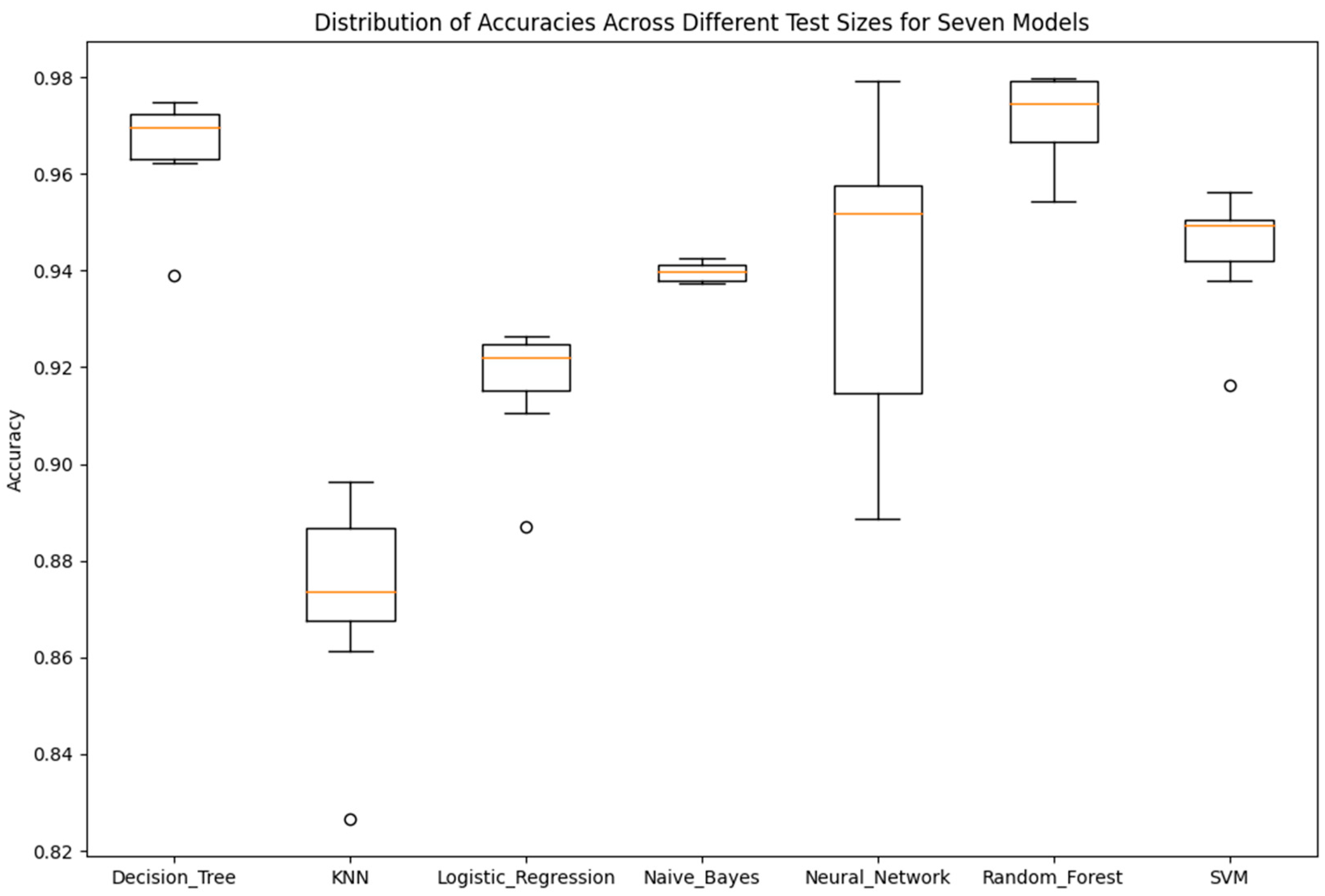
In this section, we present the results for the performance of the seven simple classifiers mentioned above. Box plots, shown in Figure 2, were utilized to demonstrate the distribution of the accuracy that each one of the seven simple classifiers achieved on the test set. The red line inside each box represents the median (50th percentile) of the data. Comparing the center lines of the box plots, we can see that the highest median is achieved by the Random Forest classifier, which suggests better average accuracy. The Decision Tree and Neural Network classifiers have also high average accuracy. The lowest accuracy is achieved by the KNN classifier. Furthermore, another key statistical measure is the Interquartile Range (IQR), which spans from the first quartile Q1 to the third quartile Q3. The height of the box indicates the spread of the middle 50% of the data. The larger the box, the more variability in the data.

As shown in Figure 2, the Neural Network classifier has the highest variability and the Naïve Bayes classifier has the lowest variability. Moreover, the lines extending from the box (whiskers) represent the range of the data. The highest range is demonstrated by the Neural Network classifier and the lowest range by the Naïve Bayes classifier. The individual points represented as dots beyond the whisker are potential outliers, i.e., cases where the model achieved unusually high or low accuracy. Except for the Naïve Bayes, Neural Network, and Random Forest classifiers, all the other models demonstrate signs of outliers. In all the cases, we observe outliers below the whisker, which means that these instances achieved lower accuracy than the majority of test cases. The results of the Naïve Bayes classifier reinforce the opinion that is generally a robust model that performs well enough in many cases despite its simplification of variables. The overall sense for the performance is that models with higher medians and less variability perform better. In our case, these include the Decision Tree, Random Forest, and Neural Network models.

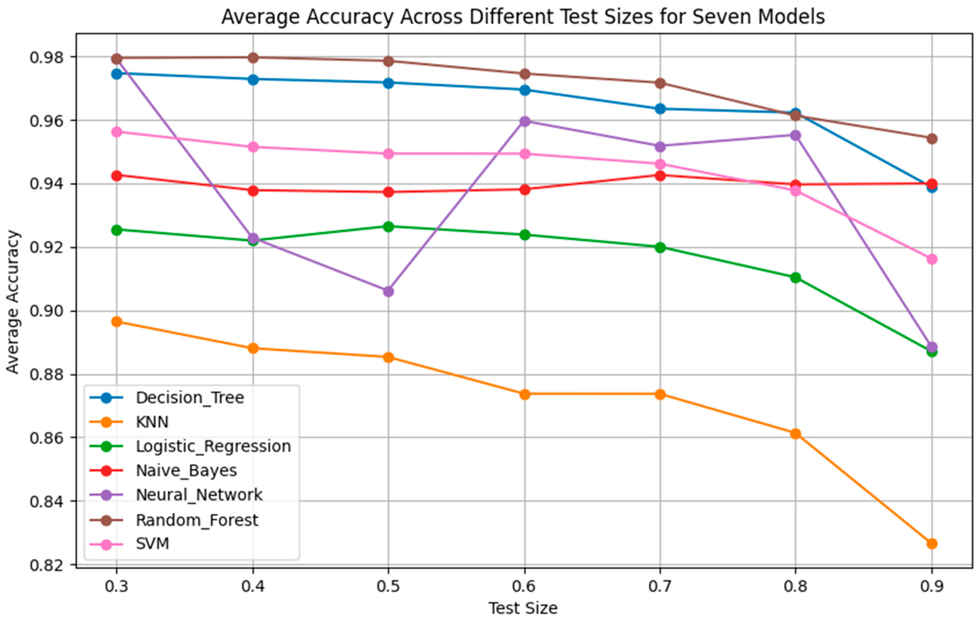
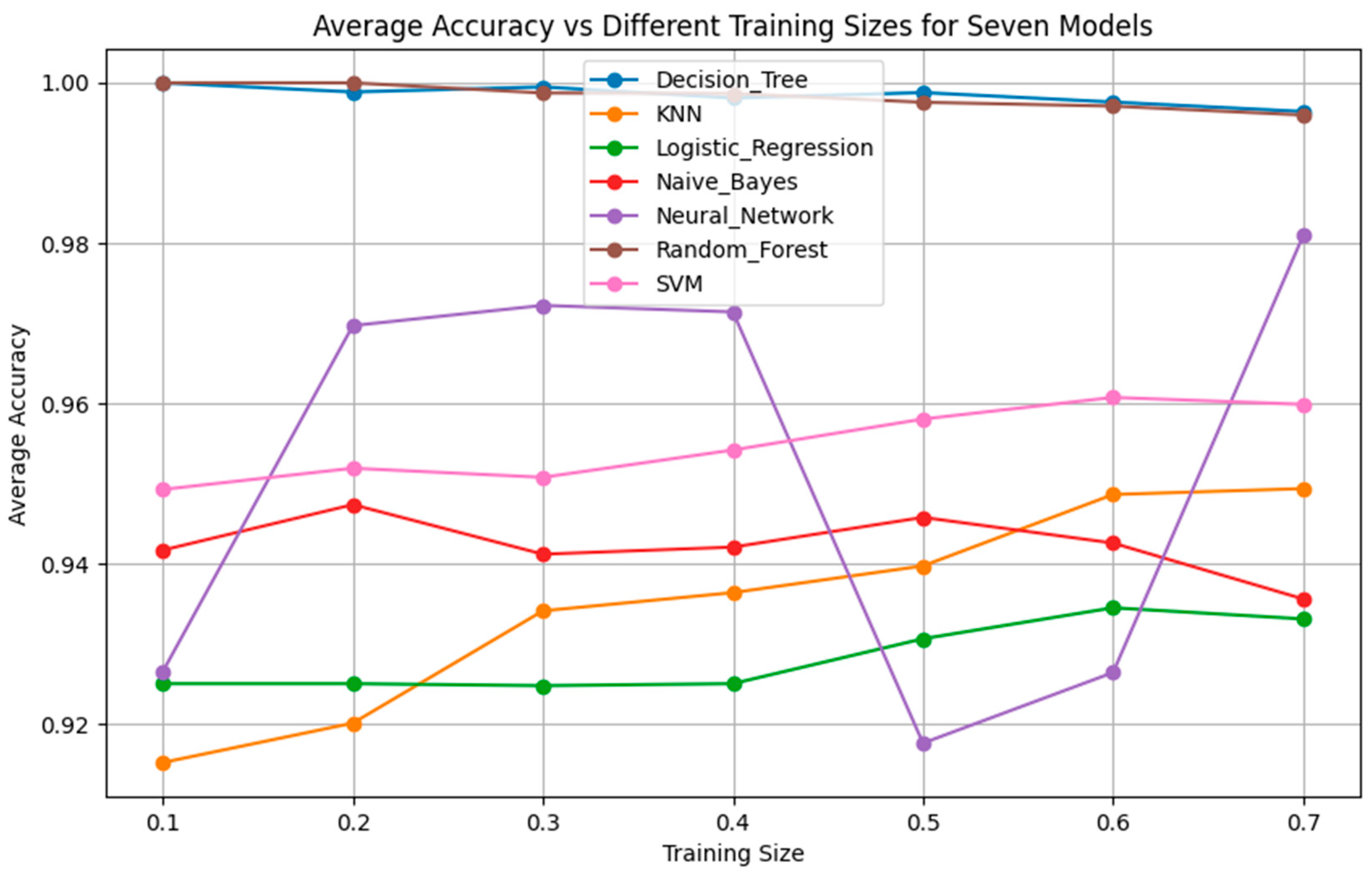
Furthermore, we implemented, with the help of Python, multiple graphical representations for all classifiers and for several values of the test set size (30–90%) and the training set size (10–70%). The obtained results are presented in Figure 3 and Figure 4, respectively. As can be seen, Decision Tree, Random Forest, and Neural Network score the highest accuracy. It is worth mentioning that for the Neural Network, the highest results were obtained when the test set size was 30% of the data, whereas Random Forest achieved the highest accuracy score when the test set size was 40% of the data and Decision Tree when the test set size was 30%. In all other cases, and especially when the test set size was 90%, the classifiers performed worst, except the Naïve Bayes model, which, in this case, achieved the best accuracy.

In addition to accuracy, additional metrics were utilized for further evaluation of the performance, i.e., Precision and Recall. Below, we give a short description of all the metrics for a better understanding of the results.

True positive (TP): the number of patients positive for biopsy predicted as positive for biopsy.

True negative (TN): the number of patients negative for biopsy predicted as negative for biopsy.

False positive (FP): the number of patients negative for biopsy predicted as positive for biopsy.

False negative (FN): the number of patients positive for biopsy predicted as negative for biopsy.

Accuracy: the proportion of test samples correctly predicted.

$$\mathrm{Accuracy}=\frac{(TP+TN)}{(TP+TN+FP+FN)}$$

Precision: the proportion of positive-for-biopsy patient predictions that were correct.

$$\mathrm{Precision}=\frac{TP}{(TP+FP)}$$

Recall: the proportion of all positive-for-biopsy patients correctly predicted.

$$\mathrm{Recall}=\frac{TP}{(TP+FN)}$$

The results of the aforementioned performance metrics are summarized in

Table 4. Performance of the seven simple classifiers with respect to accuracy, precision, and recall vs. test set size.

		Test Set Size
		0.3			0.4			0.5			0.9
Classifiers		Acc	Pre	Rec	Acc	Pre	Rec	Acc	Pre	Rec	Acc	Pre	Rec
1	Decision Tree	0.974	0.962	0.941	0.972	0.952	0.945	0.971	0.944	0.946	0.952	0.914	0.905
2	Random Forest	0.979	0.957	0.962	0.979	0.961	0.959	0.978	0.955	0.962	0.958	0.942	0.895
3	KNN	0.896	0.863	0.717	0.888	0.863	0.691	0.885	0.847	0.677	0.828	0.827	0.437
4	Logistic Regression	0.925	0.895	0.815	0.921	0.883	0.812	0.926	0.884	0.824	0.890	0.883	0.670
5	SVM	0.956	0.936	0.897	0.951	0.924	0.891	0.949	0.906	0.898	0.920	0.897	0.787
6	Naïve Bayes	0.942	0.958	0.815	0.937	0.952	0.808	0.937	0.943	0.805	0.939	0.950	0.812
7	Neural Network	0.979	0.966	0.952	0.922	0.932	0.762	0.906	0.955	0.693	0.888	0.917	0.652

, whereas, in

Table 5. Overfitting factor of the seven simple classifiers vs. test set size.

		Test Set Size vs. Training Set Size
		0.3 vs. 0.7	0.4 vs. 0.6	0.5 vs. 0.5
Classifiers		Overfit Factor	Overfit Factor	Overfit Factor
1	Decision Tree	0.025	0.026	0.027
2	Random Forest	0.019	0.019	0.019
3	KNN	0.040	0.051	0.057
4	Logistic Regression	−0.001	0.003	0.004
5	SVM	−0.006	0.003	0.009
6	Naïve Bayes	−0.001	0.005	0.008
7	Neural Network	−0.007	0.050	0.011

, the results for the overfitting factor for various combinations of the test set size and the training set size are summarized.

3.2. Performance of the Three Hybrid Classifiers

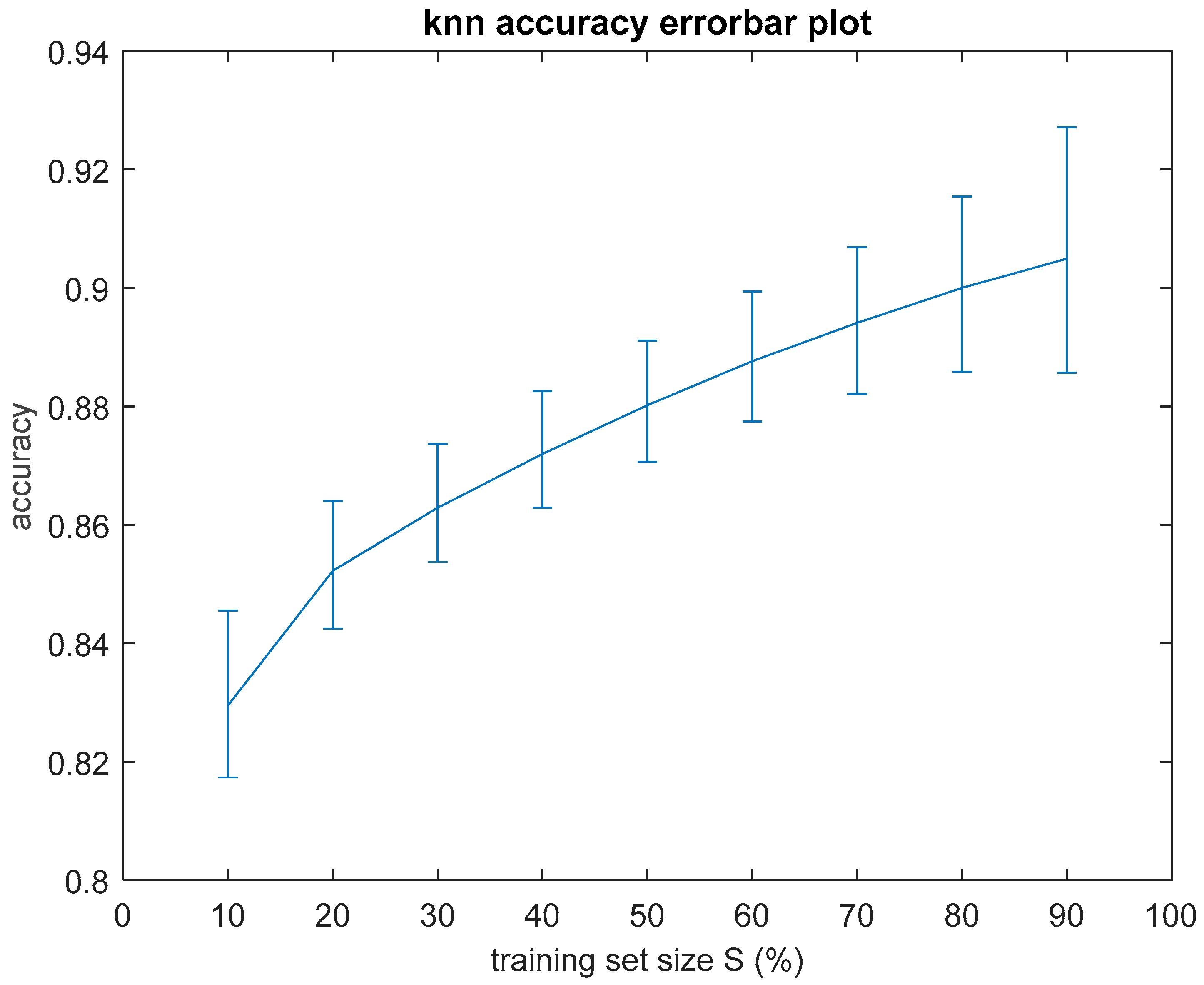
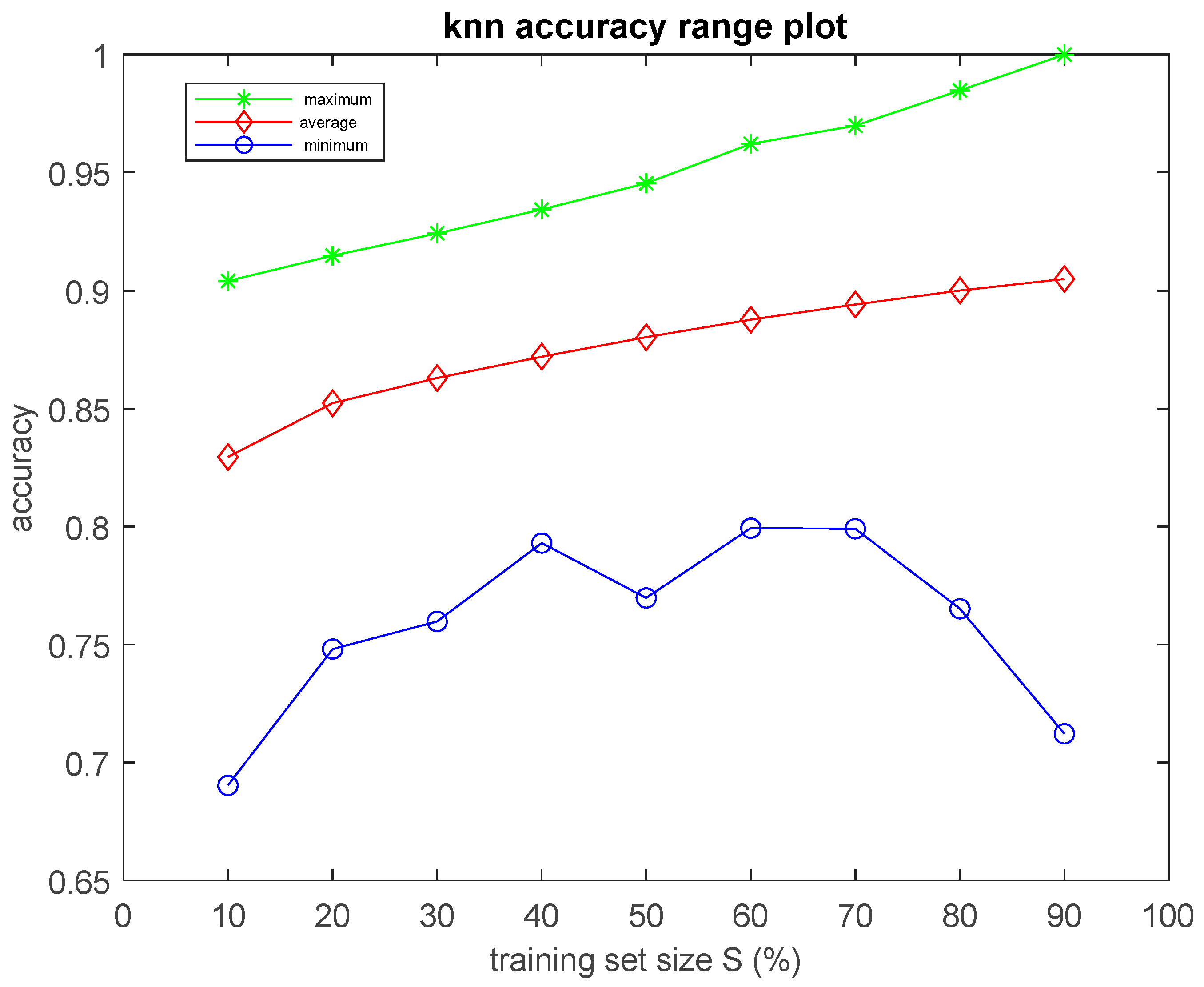
According to the results of the simple classification algorithms, KNN seems to be among the ones that present the poorest classification performance. This gave motivated us to investigate the range of classification performance of the KNN algorithm. For that purpose, 100,000 independent experiments of KNN classification were performed for various values of the training set size S.

The obtained results for k = 3 neighbors are resented in Figure 5 and Figure 6. Figure 5 presents the average values and the error bars of the classification accuracy with respect to the training set size S that was obtained for 100,000 independent experiments. In Figure 6, the corresponding maximum, minimum, and average classification accuracy values that were obtained by these 100,000 independent experiments are plotted vs. S. Figure 5 shows a strong dependence of the classification accuracy on the size S of the training set: the larger the training set, the higher the classification accuracy. In addition, as can be seen in Figure 6, despite its poor performance, the KNN classifier managed to achieve accuracy equal to 1 for training set size S = 90%. A more detailed analysis of the results revealed that an accuracy equal to 1 resulted in 98 of 100,000 experiments, that is, for approximately 0.1% of the experiments.

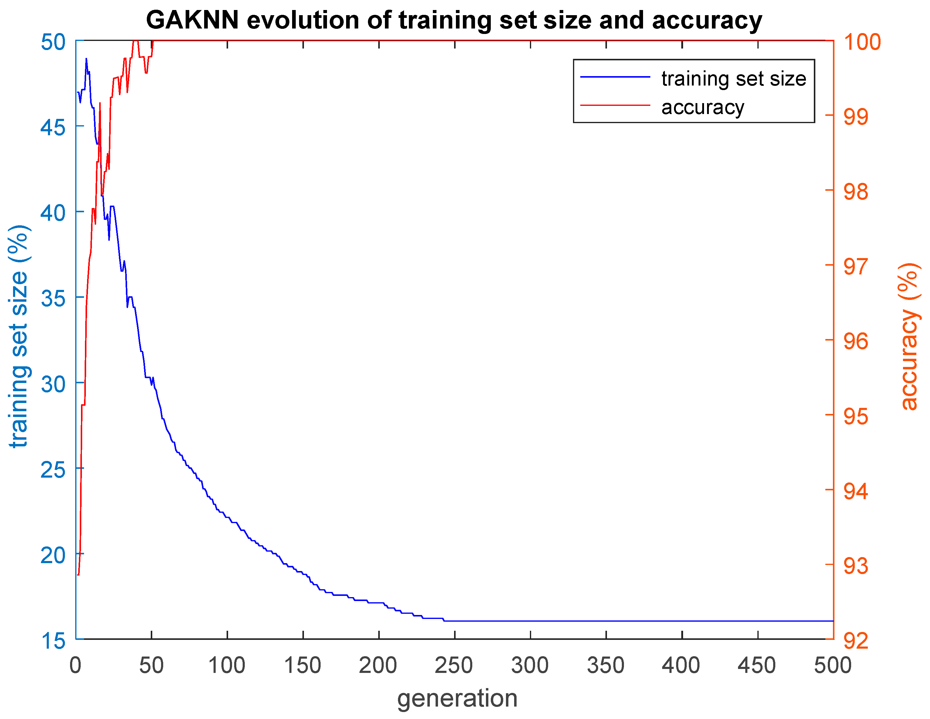
These findings led to the inquiry into the minimum size of the training set that could achieve an accuracy equal to 1 on the test set, which was realized with the use of Genetic Algorithms and the implementation of the three hybrid algorithms GAKNN, GAKMEANS, and GACLUST that were presented in Section 2.3. Representative results of the three hybrid classifiers developed in the present study are demonstrated in this section. Figure 7 shows the evolution of the training set size S of the fittest individual of each generation (blue line with respect to the right y-axis of the plot) and the corresponding classification accuracy acc of that individual (red line with respect to the left y-axis of the plot) for the GAKNN hybrid algorithm. The population of the GA consisted of 100 individuals, the crossover probability for the uniform crossover operator was set to 0.8, the mutation probability for the uniform mutation operator was set to 0.05 and the GA evolved for 500 generations. The value of the balancing factor alpha in the fitness function (Equation (2)) was set to 0.35, and the KNN algorithm was operated for k = 3 neighbors. The size of the training set gradually descended for the first 250 generations and then converged to an optimal set with size 106 (16.06% of the total 660 cases of the dataset). The classification accuracy on the test set reached its highest value (100%) in the early stage of evolution, even before the 65th generation, and consequently was maintained there.

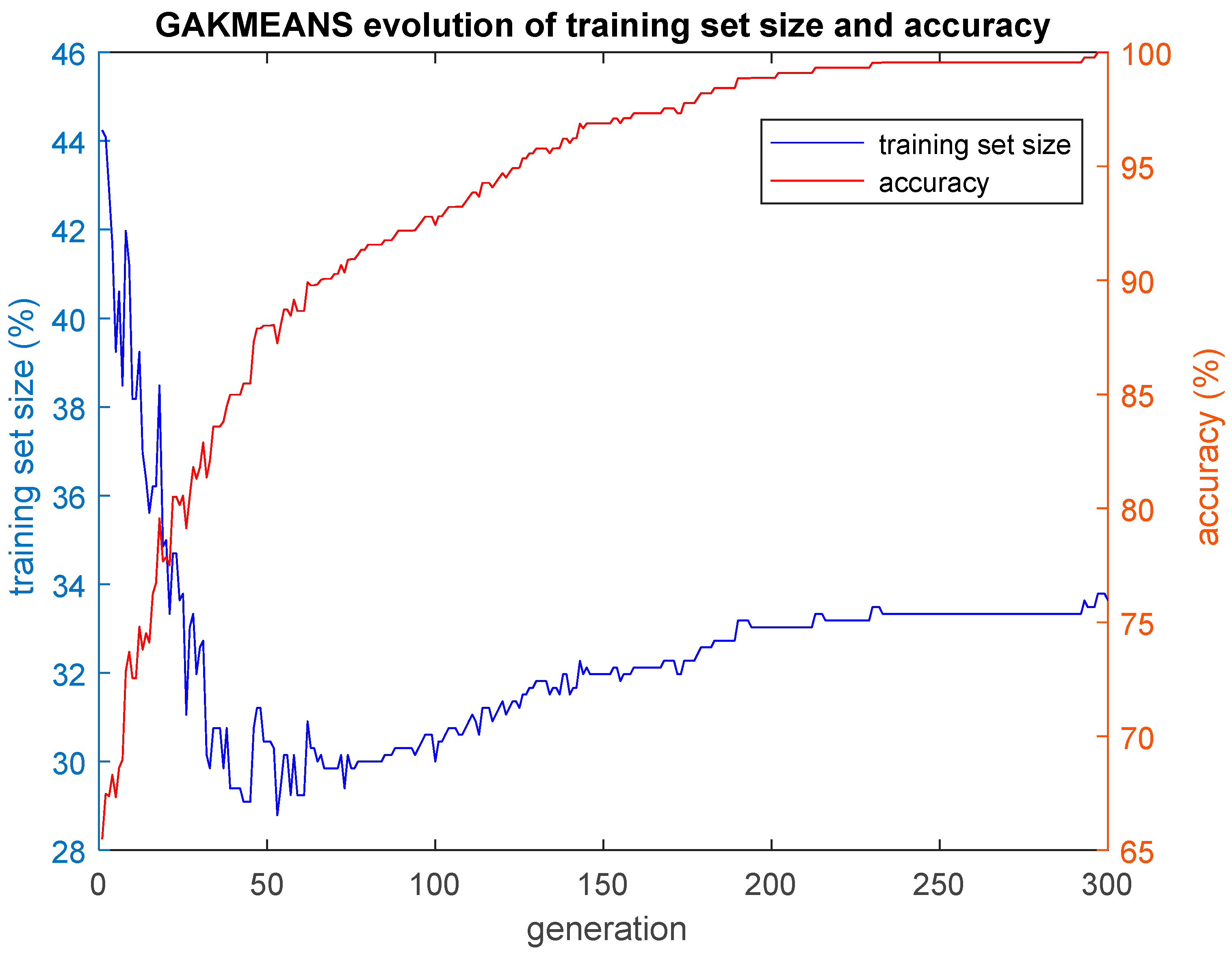
The corresponding results for the GAKMEANS hybrid classification algorithm are presented in Figure 8. Again, the evolution of the training set size S of the fittest individual of each generation is presented by the blue line with respect to the right y-axis of the plot and the evolution of the classification accuracy acc of that individual is shown by the red line with respect to the left y-axis of the plot. The population of the GA consisted of 100 individuals, the crossover probability for the uniform crossover operator was set to 0.8, the mutation probability for the uniform mutation operator was set to 0.05, and the GA evolved for 300 generations. The value of the balancing factor alpha in the fitness function (Equation (2)) was set to 0.70. The GA converged to an optimal training set with size 222 (33.64% of the total 660 cases of the dataset), while the accuracy on the test set reached its highest value (100%) in the few last generations. In Figure 8, it is important to note the way that the training set size S evolved. It clearly followed a steep descent in the first 50 generations, reaching a minimum of approximately 28.82%, but after that, it gradually increased for the next 180 generations, up to generation 230. It then converged to its final value in the few last generations at almost the end of its evolution, where the size of the training set was 33.64%. It seems like the GA was fluctuating between the two objectives that were to be optimized and, eventually, the minimization of S was sacrificed, since S increased by 4.82%, for the maximized accuracy acc of the optimal value (100%) to be achieved. Such a behavior is related to the selected value of the parameter alpha of the fitness function (Equation (2)) and can be considered as emergent behavior that implies intelligent characteristics [60,61].

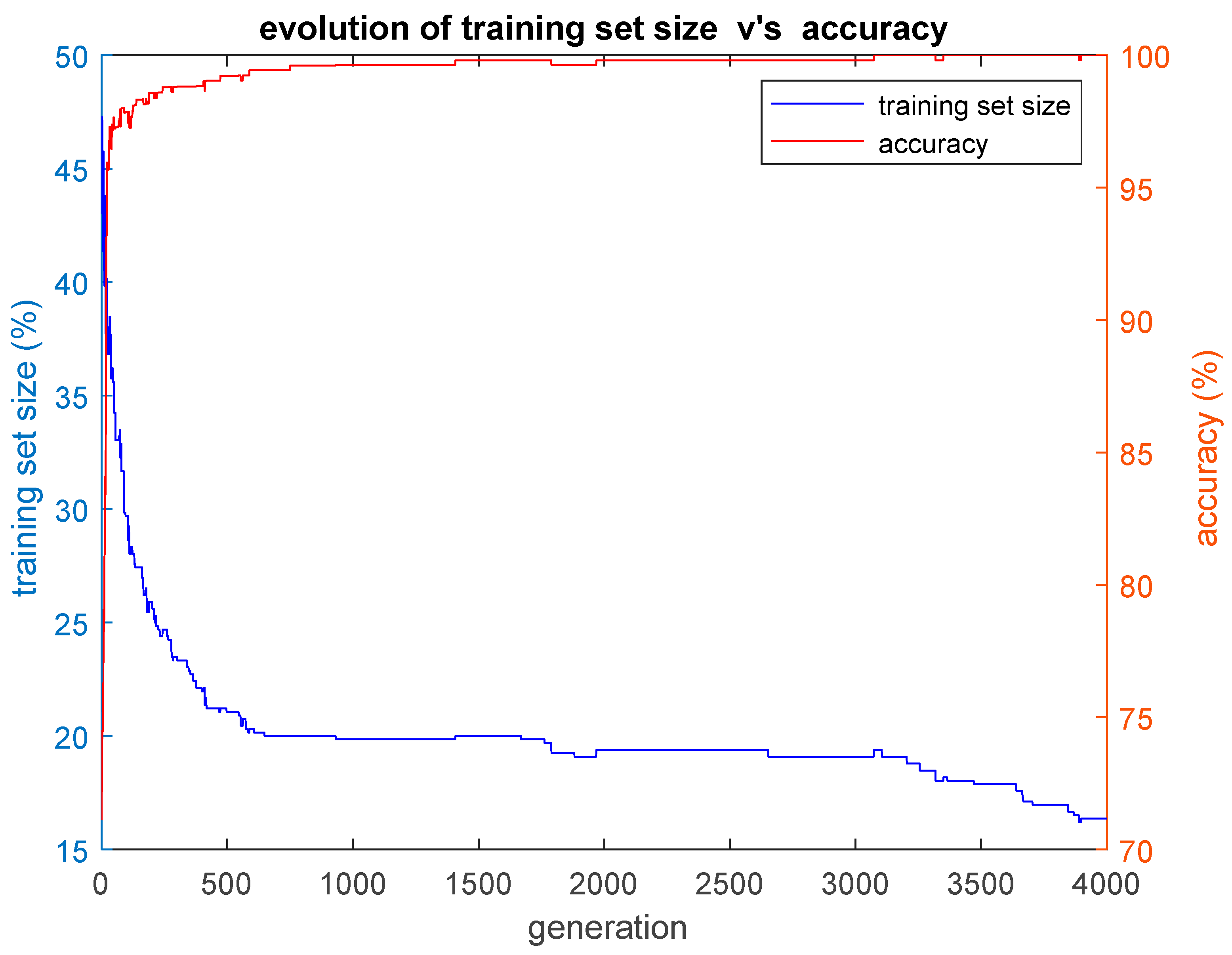
Regarding the third hybrid algorithm, representative results obtained by the GACLUST classification algorithm are shown in Figure 9, in the same manner as the ones of the two other hybrid algorithms presented above. The population of the GA consisted of 100 individuals, the crossover probability and the mutation probability were kept at 0.8 and 0.05, respectively, and the GA evolved for 4000 generations. The value of the balancing factor alpha in the fitness function (Equation (2)) was set to 0.60. According to these results, the size S of the training set rapidly decreased for the first 500 generations, reaching a value close to 20%, while, at the same time, the classification accuracy climbed close to 100%. Afterward, S descended very slowly for the next 4500 generations, moving toward a set of 108 cases (16.37% of the total cases of the dataset), while the classification accuracy on the test set finally reached its optimal value of 100%.

Table 6. Summarized, representative results of four independent computer experiments for each one of the three hybrid algorithms regarding the optimal training set for each experiment.

Algorithm	alpha	Accuracy	S	Biopsy	No Biopsy
GAKMEANS	0.80	1.00000	222	50	172
GAKMEANS	0.75	1.00000	222	50	172
GAKMEANS	0.70	1.00000	222	50	172
GAKMEANS	0.70	1.00000	224	34	210
GAKNN	0.40	1.00000	107	59	48
GAKNN	0.35	1.00000	110	62	48
GAKNN	0.35	1.00000	106	58	48
GAKNN	0.30	1.00000	110	60	50
GACLUST	0.60	1.00000	127	34	93
GACLUST	0.60	1.00000	108	41	67
GACLUST	0.50	1.00000	113	45	68
GACLUST	0.40	1.00000	125	37	88

presents a summary four representative results for each of the three hybrid algorithms. These results were obtained after conducting numerous independent computer experiments. In Table 6, the first column corresponds to the name of the hybrid algorithm; the second column corresponds to the value of the parameter alpha that was used in the fitness function of the GA, according to Equation (2); the third column presents the classification accuracy (acc) that was achieved by the fittest individual of the last generation of the GA; the fourth column presents the size S of the training set, in the number of cases, for the corresponding fittest individual; the fifth column presents the number of cases in the training set that should proceed to biopsy; and, finally, the sixth column presents the number of cases in the training set that should not proceed to biopsy. According to the findings presented in Table 6, the GAKK and GACLUST hybrid algorithms seem to achieve almost the same performance with respect to the size S of the training set. In addition, it is noteworthy that, according to Table 6, the GACLUST algorithm outperformed the GAKMEANS algorithm in terms of the size S of the training set, which is essential to achieve 100% classification accuracy on the test set. Namely, the GACLUST algorithm utilized 16.37% of the dataset to form the optimal training set, whereas the GAKMEANS algorithm utilized 33.64% of the dataset to achieve maximum classification performance. A final comment that can be made regarding the findings presented in Table 6 is that, especially in the cases of the GAKNN and the GACLUST algorithms, the pressure that the alpha factor exerts on the construction of the training set is clearer.

Finally,

Table 7. Classification results of four independent computer experiments for each one of the three hybrid algorithms regarding classification performance when a training–validation–test splitting is used on dataset 1 and a second independent test set of surrogate data is used (set 2).

Algorithm	alpha	Accuracy on Test Set 1	Accuracy on Test Set 2	S	Biopsy	No Biopsy
GAKMEANS	0.55	1.00000	1.00	234	34	200
GAKMEANS	0.60	1.00000	1.00	235	44	191
GAKMEANS	0.65	1.00000	0.98	233	44	189
GAKMEANS	0.70	0.99055	0.97	237	31	206
GAKNN	0.15	1.00000	1.00	122	64	58
GAKNN	0.20	1.00000	1.00	114	60	54
GAKNN	0.25	1.00000	0.98	124	66	58
GAKNN	0.30	1.00000	0.97	126	60	50
GACLUST	0.50	1.00000	0.96	125	66	60
GACLUST	0.55	0.99813	0.98	126	38	88
GACLUST	0.60	1.00000	0.99	123	39	84
GACLUST	0.65	0.98168	0.98	114	40	74

summarizes the obtained results for two groups of computer experiments. In the first group of experiments, the dataset of N = 660 cases that was used in all the aforementioned results (from now on referred to as set 1) was split into three subsets, namely, the training, the validation, and the test subsets, with the validation and the test subsets of equal size. This follows a widely used practice in machine learning for dataset splitting. In these experiments, the hybrid algorithms were trained with the use of the training set, and during the training procedure, the data of the validation set, as well as the data of the test set, were kept unseen. After the completion of the training procedure, the trained hybrid algorithms were evaluated with the use of the validation set and the test set. The classification accuracy achieved with the use of dataset 1 is presented in the third column of Table 7, regarding four independent computer experiments for each one of the hybrid algorithms. In the second group of experiments, the trained algorithms were evaluated with the use of a second, independently generated dataset (set 2), which consisted of 100 cases. The surrogate data in dataset 2 were generated by the same means that the surrogate dataset 1 was generated. The data in set 2 were kept unseen by the algorithms during the training procedure with the use of the data in set 1. The classification accuracy achieved on the second dataset (set 2) is presented in the fourth column of Table 7. According to Table 7, the hybrid algorithms retained their high classification performance in the first group of experiments, where dataset 1 was split in three subsets (namely, the training subset, the validation subset, and the test subset) since no significant difference was observed with respect to the corresponding results shown in Table 6, where dataset 1 was split into only two subsets (training subset and test subset). Regarding the additional evaluation of the performance of the hybrid algorithms on a second independent dataset (set 2), the algorithms proved robust and were not overfitted. Given what is shown in Table 7, with the use of approximately 30% of dataset 1 for training, all three hybrid algorithms achieved classification performance 100%, or close to that, on the remaining 70% of dataset 1 that was used for validation and testing, and at least 96% on the independent dataset 2 that was used for the second round of testing. These findings provide evidence that the proposed method for training set minimization does not lead to overfitting of the hybrid algorithms. On the contrary, it seems that the three proposed hybrid algorithms are capable of detecting the minimum training core of the dataset, i.e., the minimum training subset that can be used for training, in order to achieve high, or even perfect, performance on the training subset.

4. Conclusions

The original motivation of the present study was the fact that there is no published paper applying machine learning algorithms to classify clinical data related to the potential development of prostate cancer and to assist in decision-making by medical specialists concerning the issue of whether a patient should proceed to biopsy or not. The lack of such studies prompted us to construct surrogate data, based on a lognormal probability distribution function that presents authentic clinical PSA data reported elsewhere, and based on that, to extend our dataset in order to include additional features based on biomarkers like PSAD, PSAV, PSAR, and the DRE. These five features, combined with patient age as a sixth feature and the binary classification of the cases into two groups, i.e., those who are considered positive to proceed to biopsy and those who are negative for biopsy, formed the dataset on which the performance of seven simple classification algorithms was tested.

The simple classification algorithms that were evaluated in the present study include Decision Tree, Random Forest, Neural Networks, K-Nearest Neighbors, Logistic Regression, Naïve Bayes, and Support Vector Machines. The performance of these algorithms was examined for different sizes of the training set and the test set. The obtained results, presented in Figure 3 and Figure 4, respectively, showed that the most efficient algorithms are the Decision Tree, Random Forest, and Neural Network algorithms, which achieved a score of at least 98% average classification accuracy on the test set. However, these results revealed a strong relationship between the performance of these three algorithms (as well as the other four) and the size of the training set. This relationship was investigated in more detail (Figure 5 and Figure 6) by conducting 100,000 independent experiments for the KNN algorithm, which is among the algorithms that present the poorest performance. This investigation revealed that even the KNN algorithm can achieve 100% classification accuracy depending on the cases that constructed the training set. These findings prompted us to develop three hybrid classification algorithms for a two-objective Genetic Algorithm search (a) of the optimal training set regarding its size S and the cases that it is constructed of and (b) that, at the same time, optimizes the classification performance of the underlying classification algorithm. The classification methods in these three hybrid algorithms, namely, GAKNN, GAKMEANS, and GACLUST, were, respectively, the simple KNN classification algorithm, the simple k-means clustering algorithm, and a new genetic clustering algorithm introduced in the present work. All these three hybrid algorithms were able to detect training sets with sizes that were 16.06% of the total cases for the GAKNN algorithm, 16.37% for the GACLUST algorithm, and 33.64% for the GAKMEANS algorithm, which achieved optimal classification accuracy on the test set equal to 100%. Indicative of the improvement in the results of the hybrid algorithms is that the simple KNN algorithm, which, according to Figure 4 and Table 4 also showed accuracy below 90% even for training sets with a size of 70% of the total cases. With the use of GA optimization, it achieved a performance of 100% in classification accuracy on the test set, using only 16.06% of the cases in the training set.

Based on the preliminary though very encouraging results presented in this paper, in future work, we intend to investigate issues that were raised but not studied in the required depth in the context of this paper. These issues include (a) the performance of the remaining simple classifiers when integrated into corresponding hybrid algorithms, in the same way that the behavior of the simple KNN algorithm and the hybrid GAKNN algorithm were investigated, also considering the fine tuning of the hyper-parameters of these classifiers, for example, the number of neighbors considered in the KNN algorithms, the number of hidden neurons, the learning rate, the activation function, etc., in the ANN algorithm, and so on, (b) the performance of hybrid algorithms for more complex fitness functions including additional performance metrics such as sensitivity and specificity, (c) the role of the alpha parameter in the behavior of the fitness function (Equation (2)), as the conducted experiments indicated that the appropriate value of this parameter can improve or worsen classification performance, (d) the further investigation of the behavior of the GA from the perspective of emerging behavior, especially since it appears to involve intelligent characteristics, as it was clearly shown in the case of the GAKMEANS algorithm, and (e) given that the proposed hybrid algorithms are of general purpose, in future work, they will be applied on other datasets that are used for machine learning classification algorithms benchmarking. Last but not least, since a simple and easy-to-use GUI was developed in the context of this work, which can be used to assist in making a medical decision about whether or not to perform a prostate cancer biopsy in order for the possibility of prostate cancer to be evaluated, we intend to further enrich this environment taking into account the findings obtained from the application of hybrid algorithms of this research, as well as everything that arises in the future.

Finally, after a long reviewing procedure of the present work, the authors cordially thank all the reviewers for their constructive comments.

References

1. Casey, R.G.; Hegarty, P.K.; Conrit, R.; Rea, D.; Bytler, M.R.; Grainger, R.; McDermott, T.; Thornhill, J.A. The Distribution of PSA Age-Specific Profiles in Healthy Irish Men between 20 and 70. ISRN Oncol. 2012, 2012, 832109. [Google Scholar] [CrossRef]
2. American Cancer Society. Cancer Facts & Figures 2023; American Cancer Society: Atlanta, GA, USA, 2023; Available online: https://www.cancer.org/cancer/types/prostate-cancer/detection-diagnosis-staging/survival-rates.html (accessed on 15 December 2023).
3. Bray, F.; Ferlay, J.; Soerjomataram, I.; Siegel, R.L.; Torre, L.A.; Jemal, A. Global cancer statistics 2018: GLOBOCAN estimates of incidence and mortality worldwide for 36 cancers in 185 countries. CA Cancer J. Clin. 2018, 68, 394–424. [Google Scholar] [CrossRef]
4. Ferlay, J.E.M.; Lam, F.; Colombet, M.; Mery, L.; Pineros, M.; Znaor, A.; Soerjomataram, I. Global Cancer Observatory: Cancer Today; International Agency for Research on Cancer: Lyon, France; Available online: https://gco.iarc.fr/today (accessed on 15 December 2023).
5. Panigrahi, G.K.; Praharaj, P.P.; Kittaka, H.; Mridha, A.R.; Black, O.M.; Singh, R.; Mercer, R.; van Bokhoven, A.; Torkko, K.C.; Agarwal, C.; et al. Exosome proteomic analyses identify inflammatory phenotype and novel biomarkers in African American prostate cancer patients. Cancer Med. 2019, 8, 1110–1123. [Google Scholar] [CrossRef]
6. Ferlay, J.E.M.; Lam, F.; Colombet, M.; Mery, L.; Pineros, M.; Znaor, A.; Soerjomataram, I.; Bray, F. Global Cancer Observatory: Cancer Tomorrow; International Agency for Research on Cancer: Lyon, France; Available online: https://gco.iarc.fr/tomorrow (accessed on 15 December 2023).
7. Perdana, N.R.; Mochtar, C.A.; Umbas, R.; Hamid, A.R. The Risk Factors of Prostate Cancer and Its Prevention: A Literature Review. Acta. Med. Indones. 2016, 48, 228–238. [Google Scholar]
8. National Cancer Institue. SEER Cancer Statistics Review 1975–2013. Available online: https://seer.cancer.gov/csr/1975_2015/ (accessed on 10 December 2023).
9. Chu, L.W.; Ritchey, J.; Devesa, S.S.; Quraishi, S.M.; Zhang, H.; Hsing, A.W. Prostate cancer incidence rates in Africa. Prostate Cancer 2011, 2011, 947870. [Google Scholar] [CrossRef]
10. Hsing, A.W.; Tsao, L.; Devesa, S.S. International trends and patterns of prostate cancer incidence and mortality. Int. J. Cancer 2000, 85, 60–67. [Google Scholar] [CrossRef]
11. Gibson, T.M.; Ferrucci, L.M.; Tangrea, J.A.; Schatzkin, A. Epidemiological and clinical studies of nutrition. Semin. Oncol. 2010, 37, 282–296. [Google Scholar] [CrossRef]
12. Rohrmann, S.; Platz, E.A.; Kavanaugh, C.J.; Thuita, L.; Hoffman, S.C.; Helzlsouer, K.J. Meat and dairy consumption and subsequent risk of prostate cancer in a US cohort study. Cancer Causes Control. 2007, 18, 41–50. [Google Scholar] [CrossRef]
13. Major, J.M.; Cross, A.J.; Watters, J.L.; Hollenbeck, A.R.; Graubard, B.I.; Sinha, R. Patterns of meat intake and risk of prostate cancer among African-Americans in a large prospective study. Cancer Causes Control. 2011, 22, 1691–1698. [Google Scholar] [CrossRef]
14. Sinha, R.; Knize, M.; Salmon, C.; Brown, E.; Rhodes, D.; Felton, J.; Levander, O.; Rothman, N. Heterocyclic amine content of pork products cooked by different methods and to varying degrees of doneness. Food Chem. Toxicol. 1998, 36, 289–297. [Google Scholar] [CrossRef]
15. Kazerouni, N.; Sinha, R.; Hsu, C.H.; Greenberg, A.; Rothman, N. Analysis of 200 food items for benzo[a]pyrene and estimation of its intake in an epidemiologic study. Food Chem. Toxicol. 2001, 39, 423–436. [Google Scholar] [CrossRef]
16. Sinha, R.; Park, Y.; Graubard, B.I.; Leitzmann, M.F.; Hollenbeck, A.; Schatzkin, A.; Cross, A.J. Meat and meat-related compounds and risk of prostate cancer in a large prospective cohort study in the United States. Am. J. Epidemiol. 2009, 170, 1165–1177. [Google Scholar] [CrossRef]
17. Tappel, A. Heme of consumed red meat can act as a catalyst of oxidative damage and could initiate colon, breast and prostate cancers, heart disease and other diseases. Med. Hypotheses 2007, 68, 562–564. [Google Scholar] [CrossRef]
18. Venkateswaran, V.; Klotz, L.H. Diet and prostate cancer: Mechanisms of action and implications for chemoprevention. Nat. Rev. Urol. 2010, 7, 442–453. [Google Scholar] [CrossRef]
19. Pauwels, E.K. The protective effect of the Mediterranean diet: Focus on cancer and cardiovascular risk. Med. Princ. Pract. 2011, 20, 103–111. [Google Scholar] [CrossRef]
20. Berquin, I.M.; Min, Y.; Wu, R.; Wu, J.; Perry, D.; Cline, J.M.; Thomas, M.J.; Thornburg, T.; Kulik, G.; Smith, A.; et al. Modulation of prostate cancer genetic risk by omega-3 and omega-6 fatty acids. J. Clin. Investig. 2007, 117, 1866–1875. [Google Scholar] [CrossRef]
21. Ferris-i-Tortajada, J.; Garcia-i-Castell, J.; Berbel-Tornero, O.; Ortega-Garcia, J.A. Constitutional risk factors in prostate cancer. Actas Urol. Esp. 2011, 35, 282–288. [Google Scholar] [CrossRef]
22. el Attar, T.M.; Lin, H.S. Effect of vitamin C and vitamin E on prostaglandin synthesis by fibroblasts and squamous carcinoma cells. Prostaglandins Leukot. Essent. Fat. Acids 1992, 47, 253–257. [Google Scholar] [CrossRef]
23. Giovannucci, E.; Liu, Y.; Platz, E.A.; Stampfer, M.J.; Willett, W.C. Risk factors for prostate cancer incidence and progression in the health professionals follow-up study. Int. J. Cancer 2007, 121, 1571–1578. [Google Scholar] [CrossRef]
24. Freedland, S.J.; Aronson, W.J. Obesity and prostate cancer. Urology 2005, 65, 433–439. [Google Scholar] [CrossRef]
25. Kaaks, R.; Stattin, P. Obesity, endogenous hormone metabolism, and prostate cancer risk: A conundrum of “highs” and “lows”. Cancer Prev. Res. 2010, 3, 259–262. [Google Scholar] [CrossRef]
26. Banez, L.L.; Hamilton, R.J.; Partin, A.W.; Vollmer, R.T.; Sun, L.; Rodriguez, C.; Wang, Y.; Terris, M.K.; Aronson, W.J.; Presti, J.C.; et al. Obesity-related plasma hemodilution and PSA concentration among men with prostate cancer. JAMA 2007, 298, 2275–2280. [Google Scholar] [CrossRef]
27. Allott, E.H.; Masko, E.M.; Freedland, S.J. Obesity and prostate cancer: Weighing the evidence. Eur. Urol. 2013, 63, 800–809. [Google Scholar] [CrossRef]
28. Galdiero, M.R.; Bonavita, E.; Barajon, I.; Garlanda, C.; Mantovani, A.; Jaillon, S. Tumor associated macrophages and neutrophils in cancer. Immunobiology 2013, 218, 1402–1410. [Google Scholar] [CrossRef]
29. IAfRoC (IARC). IARC monographs on the evaluation of carcinogenic risks in human 83. In Tobacco Smoke and Involuntary Smoking; IARC Press: Lyon, France, 2004. [Google Scholar]
30. Lin, Y.; Mao, Q.; Zheng, X.; Yang, K.; Chen, H.; Zhou, C.; Xie, L. Human papillomavirus 16 or 18 infection and prostate cancer risk: A meta-analysis. Ir. J. Med. Sci. 2011, 180, 497–503. [Google Scholar] [CrossRef]
31. Sridhar, G.; Masho, S.W.; Adera, T.; Ramakrishnan, V.; Roberts, J.D. Association between family history of prostate cancer. JMH 2010, 7, 45–54. [Google Scholar]
32. Schröder, F.H.; Hugosson, J.; Roobol, M.J.; Tammela, T.L.; Ciatto, S.; Nelen, V.; Kwiatkowski, M.; Lujan, M.; Lilja, H.; Zappa, M.; et al. ERSPC Investigators. Screening and prostate-cancer mortality in a randomized European study. N. Engl. J. Med. 2009, 360, 1320–1328. [Google Scholar] [CrossRef]
33. Hugosson, J.; Carlsson, S.; Aus, G.; Bergdahl, S.; Khatami, A.; Lodding, P.; Pihl, C.G.; Stranne, J.; Holmberg, E.; Lilja, H. Mortality results from the Göteborg randomised population-based prostate-cancer screening trial. Lancet Oncol. 2010, 11, 725–732. [Google Scholar] [CrossRef]
34. Thompson, I.M.; Pauler, D.K.; Goodman, P.J.; Tangen, C.M.; Lucia, M.S.; Parnes, H.L.; Minasian, L.M.; Ford, L.G.; Lippman, S.M.; Crawford, E.D.; et al. Prevalence of prostate cancer among men with a prostate-specific antigen level ≤ 4.0 ng per milliliter. N. Engl. J. Med. 2004, 350, 2239–2246. [Google Scholar] [CrossRef]
35. Morris, P.D.; Channer, K.S. Testosterone and cardiovascular disease in men. Asian J. Androl. 2012, 14, 428–435. [Google Scholar] [CrossRef]
36. Haas, G.P.; Delongchamps, N.B.; Jones, R.F.; Chandan, V.; Serio, A.M.; Vickers, A.J.; Jumbelic, M.; Threatte, G.; Korets, R.; Lilja, H.; et al. Needle biopsies on autopsy prostates: Sensitivity of cancer detection based on true prevalence. J. Natl. Cancer Inst. 2007, 99, 1484–1489. [Google Scholar] [CrossRef]
37. Seaman, E.; Whang, M.; Olsson, C.A.; Katz, A.; Cooner, W.H.; Benson, M.C. PSA density (PSAD). Role in patient evaluation and management. Urol. Clin. N. Am. 1993, 20, 653–663. [Google Scholar] [CrossRef]
38. Loeb, S.; Metter, E.J.; Kan, D.; Roehl, K.A.; Catalona, W.J. Prostate-specific antigen velocity (PSAV) risk count improves the specificity of screening for clinically significant prostate cancer. BJU Int. 2012, 109, 508–513; discussion 513–514. [Google Scholar] [CrossRef]
39. Duran, M.B.; Dirim, A.; Ozkardes, H. The Relationship Between Prostate Biopsy Results and PSA and Free PSA Ratio Changes in Elevated Serum PSA Patients with and without Antibiotherapy. Asian Pac. J. Cancer Prev. 2020, 21, 1051–1056. [Google Scholar] [CrossRef]
40. Goldberg, D.E. Genetic Algorithms in Search, Optimization, and Machine Learning, 1st ed.; Addison-Wesley: Boston, MA, USA, 1989. [Google Scholar]
41. Weisstein, E.W. Random Walk—1-Dimensional. MathWorld. Available online: https://mathworld.wolfram.com/RandomWalk1-Dimensional.html (accessed on 27 October 2023).
42. Kissell, R.; Poserina, J. Optimal Sports Math, Statistics, and Fantasy; Elsevier: London, UK, 2017. [Google Scholar]
43. Available online: https://numpy.org/ (accessed on 1 May 2023).
44. Arneth, B.M. Clinical Significance of Measuring Prostate-Specific Antigen. Lab. Med. 2009, 40, 487–491. [Google Scholar] [CrossRef]
45. Lepor, H. Evaluating men with benign prostatic hyperplasia. Rev. Urol. 2004, 6 (Suppl. S1), 8–15. [Google Scholar]
46. Nordstrom, T.; Akre, O.; Aly, M.; Gronberg, H.; Eklund, M. Prostate-specific antigen (PSA) density in the diagnostic algorithm of prostate cancer. Prostate Cancer Prostatic Dis. 2017, 21, 57–63. [Google Scholar] [CrossRef]
47. Aminsharifi, A.; Howard, L.; Wu, Y.; De Hoedt, A.; Bailey, C.; Freedland, S.; Polascik, T. Prostate Specific Antigen Density as a Predictor of Clinically Significant Prostate Cancer When the Prostate Specific Antigen is in the Diagnostic Gray Zone: Defining the Optimum Cutoff Point Stratified by Race and Body Mass Index. J. Urol. 2018, 200, 758–766. [Google Scholar] [CrossRef]
48. Benson, M.C.; Whang, I.S.; Pantuck, A.; Ring, K.; Kaplan, S.A.; Olsson, C.A.; Cooner, W.H. Prostate specific antigen density: A means of distinguishing benign prostatic hypertrophy and prostate cancer. J. Urol. 1992, 147 Pt 2, 815–816. [Google Scholar] [CrossRef]
49. Djavan, B.; Zlotta, A.; Kratzik, C.; Remzi, M.; Seitz, C.; Schulman, C.C.; Marberger, M. PSA, PSA density, PSA density of transition zone, free/total PSA ratio, and PSA velocity for early detection of prostate cancer in men with serum PSA 2.5 to 4.0 ng/mL. Urology 1999, 54, 517–522. [Google Scholar] [CrossRef]
50. Laino, C. New Data on How Age-Adjusted PSA Velocity Can Improve Prostate Cancer Detection in Different Settings. Oncol. Times 2006, 28, 37–38. [Google Scholar] [CrossRef]
51. Christensson, A.; Björk, T.; Nilsson, O.; Dahlén, U.; Matikainen, M.-T.; Cockett, A.T.; Abrahamsson, P.-A.; Lilja, H. Serum prostate specific antigen complexed to alpha 1-antichymotrypsin as an indicator of prostate cancer. J. Urol. 1993, 150, 100–105. [Google Scholar] [CrossRef]
52. Quinn, J.; Zeleny, T.; Rajaratnam, V.; Ghiurluc, D.-L.; Bencko, V. Debate: The per rectal/digital rectal examination exam in the emergency department, still best practice? Int. J. Emerg. Med. 2018, 11, 20. [Google Scholar] [CrossRef]
53. Available online: https://scikit-learn.org/stable/ (accessed on 1 May 2023).
54. Cover, T.; Hart, P. Nearest neighbor pattern classification. IEEE Trans. Inf. Theory 1967, 13, 21–27. [Google Scholar] [CrossRef]
55. Lee, T.H.; Ullah, A.; Wang, R. Bootstrap Aggregating and Random Forest. In Macroeconomic Forecasting in the Era of Big Data. Advanced Studies in Theoretical and Applied Econometrics, 1st ed.; Fuleky, P., Ed.; Springer: Cham, Switzerland, 2020; Volume 52, pp. 389–429. [Google Scholar]
56. Edgar, T.W.; Manz, D. Exploratory Study. In Research Methods for Cyber Security, 1st ed.; Edgar, T.W., Manz, D., Eds.; Syngress: Oxford, UK, 2017; pp. 95–130. [Google Scholar]
57. Zhang, H. The Optimality of Naive Bayes. In Proceedings of the FLAIRS2004 Conference 2004, Miami Beach, FL, USA, 17–19 May 2004. [Google Scholar]
58. Appakaya, S.B.; Pratihar, R.; Sankar, R. Parkinson’s Disease Classification Framework Using Vocal Dynamics in Connected Speech. Algorithms 2023, 16, 509. [Google Scholar] [CrossRef]
59. Available online: https://www.gradio.app/ (accessed on 1 May 2023).
60. Forrest, S.; Miller, J.H. Emergent behavior in classifier systems. Phys. D Nonlinear Phenom. 1990, 62, 213–227. [Google Scholar] [CrossRef]
61. Hillis, W.D. Intelligence as an Emergent Behavior; or, The Songs of Eden. Daedalus 1988, 111, 175–189. [Google Scholar]
Figure 1. Utilized simple classifiers.
Algorithms 17 00236 g001
Figure 2. Box plots for the performance of the seven simple classifiers on the test set.
Algorithms 17 00236 g002
Figure 3. Multiple plots for the average accuracy for the seven simple classifiers vs. the size of the test set.
Algorithms 17 00236 g003
Figure 4. Multiple plots for the average accuracy for the seven classifiers vs. the size of the training set.
Algorithms 17 00236 g004
Figure 5. Average values and error bars for KNN classification accuracy vs. the size S of the training set for 100,000 independent experiments.
Algorithms 17 00236 g005
Figure 6. Range plot for KNN classification performance vs. the size S of the training set for 100,000 independent experiments. Maximum performance in green, minimum performance in blue, and average performance in red.
Algorithms 17 00236 g006
Figure 7. Evolution of the training set size S and classification accuracy on the test set for the GAKNN hybrid algorithm.
Algorithms 17 00236 g007
Figure 8. Evolution of the training set size S and classification accuracy on the test set for the GAKMEANS hybrid algorithm.
Algorithms 17 00236 g008
Figure 9. Evolution of the training set size S and classification accuracy on the test set for the GACLUST hybrid algorithm.
Algorithms 17 00236 g009