Solar Irradiance Forecasting with Natural Language Processing of Cloud Observations and Interpretation of Results with Modified Shapley Additive Explanations

Abstract

Forecasting the generation of solar power plants (SPPs) requires taking into account meteorological parameters that influence the difference between the solar irradiance at the top of the atmosphere calculated with high accuracy and the solar irradiance at the tilted plane of the solar panel on the Earth’s surface. One of the key factors is cloudiness, which can be presented not only as a percentage of the sky area covered by clouds but also many additional parameters, such as the type of clouds, the distribution of clouds across atmospheric layers, and their height. The use of machine learning algorithms to forecast the generation of solar power plants requires retrospective data over a long period and formalising the features; however, retrospective data with detailed information about cloudiness are normally recorded in the natural language format. This paper proposes an algorithm for processing such records to convert them into a binary feature vector. Experiments conducted on data from a real solar power plant showed that this algorithm increases the accuracy of short-term solar irradiance forecasts by 5–15%, depending on the quality metric used. At the same time, adding features makes the model less transparent to the user, which is a significant drawback from the point of view of explainable artificial intelligence. Therefore, the paper uses an additive explanation algorithm based on the Shapley vector to interpret the model’s output. It is shown that this approach allows the machine learning model to explain why it generates a particular forecast, which will provide a greater level of trust in intelligent information systems in the power industry.

1. Introduction

The development of distributed generation (DG) is aimed at generating electrical energy near the point of its consumption and introducing energy sources with relatively low power and compact dimensions. Typically used are installations running on diesel or gas and renewable energy sources (RES) such as photovoltaic/solar power plants (SPP), wind power plants and mini-hydroelectric power plants.

DG is especially important for supplying energy to small settlements in geographically remote areas (Arctic, mountainous, etc.) where, for technical and economic reasons, it is impossible to connect users to the general energy system and guarantee the effective centralised control of network modes [1,2].

However, when compiling power balances for energy districts with DGs based on RES, the generation forecasting problem arises; this is especially aggravated in the absence of redundancy, when the power station operates in an isolated mode from a large power system [3,4]. Partially, the problem of discrepancies in power balances can be solved by means of energy storage systems based on batteries, but the capacity of such systems is significantly lower than the possible deviations of actual generation from the forecast. Capacity expansion is limited by economic feasibility due to the high cost of energy storage systems.

There are several main groups of time series forecasting methods that are used for renewable energy sources [5]:

(1)

Numerical weather prediction (NWP);

(2)

Statistical methods;

(3)

Artificial intelligence methods.

The first group of models uses a lot of meteorological data and complex models of atmospheric movement [6]. Studies like [7] offer methods for assessing the influence of clouds, ambient temperature and other factors on the generation of photovoltaic power plants. This approach places heavy demands on the volume and quality of meteorological data, thereby often including the need to use satellite imagery or data from an extensive network of multiple weather stations. In addition, it has very high computational complexity.

On the contrary, statistical methods are much simpler and, in general, can be applied in the presence of retrospective data only on the predicted value, that is, the level of insolation or SPP generation. The most frequently used autoregressive models are autoregressive (AR), autoregressive integrated moving average (ARIMA), and their modifications [8,9]. However, the problem under consideration can only be solved with high accuracy by taking into account many meteorological factors and complex dependencies that are non-stationary within a day and over longer intervals. Static methods are not effective enough in this case.

Due to the complexity and high cost of NWP and the lack of accuracy of statistical models, machine learning models are widely used. These models can analyse multiple input factors. In this case, models based on artificial neural networks [5,10] and ensemble models [3,11,12] can be distinguished. Deep neural network models have been implemented to model and forecast solar irradiance data with the use of meteorological and geographic parameters [13,14,15].

Many studies have compared the accuracy obtained by different models. Below are examples of such work.

In article [16], hourly solar irradiance was predicted for five weather stations using four years of data, applying models based on support vector regression (SVR), decision trees (DTs), and multi-layer perceptron (MLP). Also, for each of the models, a bagging or gradient boosting algorithm was used. The authors demonstrated an improvement in forecast accuracy when using ensemble methods: the quality of models relative to basic predictors in the context of the root mean squared error increased on average from 5% to 12%, and the fitting speed increased by 7–10%. The best performance was achieved with MLP-boosting/MLP-bagging/DT-boosting (coefficient of determination R² from 0.95 to 0.97).

On the basis of solar irradiance and meteorological factors data for 2.5 years, study [17] proposed to forecast hourly irradiance with MLP, having previously analysed the dataset with k-means clustering. In comparison with linear regression (LR), DT and DT-boosting neural network improved the coefficient of determination to 0.83.

The authors of [18] used the long short-term memory (LSTM) architecture for forecasting solar panel generation. The achieved error of solar panel generation forecasting with a 15-min horizon was less than 5%.

In article [19], forecast models for SPPs based on hourly measurements of various components of insolation, air temperature, wind speed and pressure were proposed for the day ahead based on SVR, DTs, DT ensembles, and swarm intelligence (Grey wolf optimisation).

In study [20], for the hourly forecasting of solar irradiance for four years, models based on the LSTM, SVR and MLP algorithms were proposed, though the required parameters were first selected with the LASSO algorithm. The basic forecast models were additionally combined with the methods for quantile regression averaging and convex optimisation (COpt); the best base model was MLP, and the best combining algorithm was COpt.

The authors of [21] proposed to forecast the generation of SPPs based on five years of data by neural networks; the Flocking algorithm was used to optimise the parameters of the resulting models, and the neural networks themselves were subsequently ensembled by bagging. As a result, the root mean squared error of the ensemble neural network (ENN) was 8% to 12% smaller relative to the basic models.

Article [22] proposed short-term generation forecasting models based on SVR and extreme learning machine (ELM) algorithms: both models showed high accuracy (R² above 0.95), and the forecast error was 5–7%.

Study [23] proposed to apply the k-means algorithm to cluster meteorological conditions and train a separate model for each cluster using a dataset of 35 years. The best result was obtained for MLP; the forecast error for an hour ahead was 8.6% with an R² of 0.96.

A comprehensive review [10] of the use of machine learning methods for forecasting solar irradiance in various parts of the world showed that ensemble models and neural networks are the most popular tools used to solve this problem. For data pre-processing, clustering and models based on a mixture of Gaussian distributions are used. The forecast error for various planning horizons ranges from 3% to 20%.

An analysis of existing works shows that the accuracy of solar irradiance forecasting is largely influenced by the composition and quality of meteorological data. Solar radiation on clear days can be predicted with high accuracy, even in the midterm [2,23]. For cloudy days, the accuracy is significantly lower, even for a short-term forecast. Cloudiness introduces a significant difference between the solar irradiance at the top of the atmosphere calculated with high accuracy and its value on the Earth’s surface. The cloud cover can be very changeable; it complicates the task of solar irradiance forecasting.

An important feature of cloudiness, in contrast to air temperature, wind speed, precipitation intensity and most other meteorological factors, is a much less formalised form of measurement. Clouds can have different densities and heights. The frequently used measure total cloud amount does not take this into account and only shows the percentage of the sky covered by any type of cloud. In most cases, at present and even more so in the past, cloud data are the results of visual subjective observation from the Earth’s surface [24,25]. This article proposes an algorithm for formalising cloud descriptions in natural language, thereby allowing them to be converted into categorical features suitable for the use of machine learning.

In addition, it should be noted that at present, research in the field of forecasting SPP generation is still primarily aimed at increasing the accuracy of forecasts, while the models remain black boxes for users. This makes it difficult to implement machine learning predictive models in enterprises, since users want to understand why the model generates a particular forecast. To solve this problem, research is being conducted in the field of explainable artificial intelligence (XAI) [26,27]. For complex models that are not interpretable, a posteriori explanation can be used, currently represented mainly by algorithms such as local interpretable model-agnostic explanations (LIMEs) [28] and Shapley additive explanations (SHAPs) [29]. The application of LIME and SHAP methods in the power industry is still at an early stage. For example, in article [30], both methods were used to forecast SPP generation. However, the authors only used one feature relating to cloudiness. All resulting interpretations were dominated by two a priori obvious features: direct solar radiation and the hour of the day. Thus, the explanation provides the user with little new information to understand the model operation.

Our contributions to the state of the art are as follows:

• An algorithm of processing cloud observations in natural language for machine learning applications in forecasting SPP generation is proposed;
• It is experimentally substantiated that the use of different features describing the cloudiness increases the accuracy of SPP generation forecasting;
• A comparative analysis of various algorithms for constructing decision tree ensembles in SPP generation forecasting with many categorical features is carried out;
• The possibility of increasing the interpretability of SPP generation forecasts with a modified SHAP algorithm is investigated. The modification consists of combining a number of features that have close meaning for a user during visual interpretation.

In addition, the article describes real data pre-processing in detail, taking into account such features as discrete time discrepancies, omissions, and various data storage formats. A description of data pre-processing may be of interest to researchers faced with similar problems when processing data obtained from real power industry enterprises with low levels of digitalisation when collecting, processing and storing data.

The remainder of the paper is organized as follows. Section 2 presents descriptions of the object under study as well as the proposed data pre-processing algorithm, machine learning models and approach for results’ interpretation. Section 3 shows the results of applying various machine learning models to a pre-processed dataset. In Section 4, the paper is concluded with the scope of future work.

2. Materials and Methods

2.1. The SPP under Consideration

One of the SPPs located in the Altai, which has high solar energy potential [31], was chosen as the object under consideration. Until the beginning of the 2010s, the Altai Republic was a completely energy-deficient region, and generation was represented locally. Electricity was only generated at ten small diesel and wind power plants, as well as two mini-hydroelectric power plants with a total capacity of 1.3 MW, intended for the local power supply of facilities in hard-to-reach and remote settlements in the mountainous regions of the Republic, which were not connected to the general energy system. Then, the high potential of solar energy led to the creation of SPPs for the promotion of the power system with DG.

Due to data from meteorological stations, such as daily/monthly/annual sums of total solar irradiance, direct (on horizontal plane) and diffuse irradiance, and the amount of cloud cover and duration of sunshine, it was possible to obtain quantitative estimates of the solar energy potential in this area as follows:

• Average annual value of total solar radiation of 1495 kWh/m²;
• Average annual value of total cloudiness of 5.9 points with a maximum of 10 points;
• Average annual cloudiness of the lower level of 2.6 points;
• Average number of hours of sunshine per year of 2823 h, though it has reached 3000 h or more in some years;
• Solar resources for the total calendar year of 1482 kWh/m².

The SPP under consideration operates in parallel with the power system and has two parts with a nominal power of 5 MW each. Photovoltaic modules are oriented to the south, mounted on inclined surfaces at an angle of 45° to the horizon.

2.2. Initial Dataset

At the stages of searching and accumulating data, we obtained primary data on the generation of the SPP, solar irradiance at its location, and consumption by feeders at the nearest substation, which consisted of several Microsoft Office Excel Spreadsheet (version 2021) files (XLSX) with a time series of various discreteness levels.

At the same time, data on weather and climatic factors were taken from the weather archive of the open meteorological database RP5 and covered the period from 1 January 2019 to 23 February 2022 with a resolution of 180 min (three hours). Then, NASA open data of solar irradiance at the top of the atmosphere on a plane normal to the incident radiation were added to the dataset.

Table 1. List of basic data in the original uncleaned and unsorted files.

File Id	Period, dd.mm.yyyy	Time Resolution, min	Data Type
1	28 October 2019–31 December 2020	60	Solar irradiance
2	01 January 2019–31 December 2020	60	SPP generation
3	28 October 2019–31 December 2020	30	Power consumption
4	06 May 2021–30 September 2021	30	Power consumption
5	01 January 2021–30 September 2021	60	SPP generation
6	01 October 2022–23 February 2022	30	Power consumption
7	01 October 2022–23 February 2022	60	SPP generation

provides a list of the main data in the original raw and unsorted files.

Table 2. Meteorological factors.

Parameter	Parameter Description	Unit/Format
Time	Local time	dd.MM.yy hh:mm
T	Air temperature at a height of 2 m above the Earth’s surface (in this table, all heights are measured from the surface of the Earth)	°C
Po	Atmospheric pressure at station level	mm Hg
P	Atmospheric pressure normalised to mean sea level	mm Hg
Pa	Pressure trend: atmospheric pressure fluctuations over the last three hours	mm Hg
U	Relative humidity at a height of 2 m	%
DD	Wind direction at a height of 10–12 m	text description (text)
Ff	Wind speed at a height of 10–12 m	m/s
ff10	Maximum wind gust at a height of 10–12 m	m/s
ClCover	Total cloudiness	% + text
LowLevelCl	Stratocumulus clouds, stratus clouds, cumulus clouds and cumulonimbus clouds (lower clouds—up to 2 km in mid-latitudes)	text
AmountLowLevCl	Number of observed low-level clouds; the level of medium clouds in their absence	% + text
ClCeil	Height of the base of the lowest clouds	m + text
MidLevCl	Altocumulus clouds, altostratus clouds, nimbostratus clouds (mid-level clouds—from 2 km to 6 km in mid-latitudes)	text
HighLevCl	Cirrus clouds, cirrocumulus clouds and cirrostratus clouds (cloud tops—from 6 km to 13 km in mid-latitudes)	text
VV	Horizontal visibility range	km
Td	Dew point temperature at a height of 2 m	°C
RRR	Amount of precipitation	mm
tR	Period of time during which the specified amount of precipitation was accumulated	h
E	Condition of the soil surface without snow or measurable ice cover	text
Tg	Minimum soil surface temperature overnight	°C
E’	Condition of the soil surface with snow or measurable ice cover	text
sss	Snow depth	cm

presents the initial meteorological features (readings from weather station No. 36259). The dimensions of the original array are 9206 rows and 29 columns (Table 2 omits some of them, which are obviously not information-bearing for the problem being solved).

When combining and subsequently cleaning the accumulated raw data in relation to the object under consideration, problems specific to these data were identified:

• Data on generation, solar irradiance, consumption, and weather features have different time ranges of coverage;
• Weather data have a lot of missing values;
• Some of the names of the attribute columns are absolutely non-informative in the context of the real electrical circuit of the station (for example, feeders are represented by telemetering points, not by the names or numbers of outgoing power lines);
• The time resolutions of the data obtained for generation, solar irradiance, consumption, and weather data are different and range from thirty minutes to three hours;
• The volume of data for various components represents time series with several thousand, and sometimes tens of thousands, of values.

2.3. Data Aggregation and Filtering

After combining and cleaning the data, a dataset that contained 2533 records (rows) about solar irradiance, temperature, cloudiness (with various factors), and SPP generation in the period from 6 May 2020 to 23 February 2022 with a resolution of three hours was obtained.

The calculation of the volume of lost data when creating the final dataset is given in

Table 3. Amount of high-quality data lost when creating the dataset.

Dataset	Initial Number of Records	Due to Mismatched time Ranges (Records/% of Total)	Due to the Reduction of Data to One Hour Discreteness (Records/% of Total)	Due to the Discarding of Hours with Zero Generation of SPP (Records/% of Total)	Due to the Reduction of Data to a Weather Discreteness of Three Hours (Records/% of Total)
Generation	27,600	11,784/42.7%	–	9490/34.3%	3793/13.7%
Insolation	20,401	4584/22.5%	–	9490/46.5%	3793/18.6%
Consumption	31,633	–	15,817/50%	9490/30.0%	3793/12.0%
Weather	9087	3928/43.2%	–	2626/28.9%	–

. Due to the reduction of data to the latest date (6 May 2020), in order to obtain the intersection of all samples, it was already necessary at this stage to abandon 491 days of generation and weather data records on climatic factors (without irradiance), as well as from 191 days of insolation data records. Also, due to the need to bring the data to a lower resolution (one hour), records of consumption on feeders at time stamps xx:30 (hours:minutes) had to be excluded from the final dataset. Then, we excluded records in which the power generated by the SPP was 0 (since such records are not informative for forecasting) and intersected the obtained data with the weather data, which were taken from 07:00 with a resolution of three hours. Therefore, in the non-zero SPP generation interval, hits from three to five weather description hours (07:00/10:00/13:00/16:00/19:00) and the remaining six to eight hours (08:00/09:00/11:00/12:00/14:00/15:00/17:00/18:00) were discarded.

Features were classified according to Figure 1. A correlation analysis allowed us to exclude some of the less informative meteorological features: Po, P, Pa, U, DD, Ff, ff10, VV, Td, RRR, tR, E, Tg, E’, and sss.

2.4. Feature Transformation

Two new variables were identified: “Day of Year” and “Hour of Year”. These are responsible for the ordinal number of the day in the year and the ordinal number of the hour of the day, respectively.

Many machine learning algorithms require class labels to be encoded as integer values. There are many different ways to encode class labels. This work used the one-hot encoding algorithm, the idea of which is to create a new pseudo-feature for each unique value in the quality attribute column.

For the considered dataset, all unique values of cloud parameters (LowLevCl, AmountLowLevCl, MidLevCl and HighLevCl) given in

Table 4. Types of cloud descriptions and their designations.

Designation	Category	Description
NoCloud	Low, Middle, High	No clouds recorded
Sc	Low	Stratocumulus clouds
St	Low	Stratus clouds
Cb	Low	Cumulonimbus clouds
CuHum	Low	Cumulus flat clouds
CuFrac	Low	Cumulus fractus clouds
CiUnc	High	Cirrus claw clouds
CiSpissFromCb	High	Dense cirrus clouds emerging from cumulonimbus ones
CuMed	Middle	Cumulus mediocris
CuCong	Low	Cumulus congestus clouds
CbInc	Low	Cumulonimbus filament clouds (anvil cloud)
CbCalv	Low	Cumulonimbus calvus
Frnb	High	Fractonimbus clouds
StNeb	Low	Stratus nebulosus
StFra	Low	Layered fractus clouds
As	Mid	Alto-stratus clouds
ScNonCu	Low	Stratocumulus clouds that did not originate from cumulus clouds
Ci	High	Spindrift clouds
Cc	High	Cirrocumulus clouds
Cs	High	Cirrostratus clouds
AcFromCu/Cb	Mid	Altocumulus clouds originating from cumulus clouds (or cumulonimbus clouds)
ScFromCu	Low	Stratocumulus clouds originating from cumulus clouds
CiSpissInt	High	Cirrus dense curled clouds
CiCast	High	Spindrift castellanus clouds
CiFl	High	Cirrus floccus
Cu	Low	Cumulus clouds
CiFibr	High	Cirrus fibratus

were presented with unitary coding.

Since the values about cloudiness in the original dataset are in the natural language format, the pre-processing algorithm should be developed carefully. It can be presented as follows:

(1)

Convert all characters to lower case;

(2)

Replace punctuation marks and the symbols ‘_’, ‘+’, and ‘-’ with spaces;

(3)

Apply tokenisation;

(4)

Apply stemming.

For stemming, we proposed to apply the Porter algorithm [32].

As a result, phrases such as “cumulus clouds”, “Cumulus cloud”, “cumul. cloud.”, and “cumulus-clouds” turn into the identical “cumul cloud”. In addition, values with negations were removed (“not observed…”, “absent…”, “no…”), since only features characterising the presence of a particular type of cloud were used.

Preliminary experiments showed that using all cloud types (Table 4) separately did not improve forecasting accuracy, so many types were combined:

• LowCb: Cb, CbInc, and CbCalv;
• LowCu: Cu, CuHum, CuFrac, and CuCong;
• LowSt: St, Sc, StNed, StFrac, ScNonCu, and ScFromCu;
• Mid: CuMed, As, and AcFromCu/Cb;
• HiS: CiSpissFromCb, and CiSpissInt;
• HiFrnb: Frnb;
• HiCi: Ci, Cc, Cs, CiUnc, CiCast, CiFl, and CiFibr.

The algorithm for converting cloud records is given below (Algorithm 1). As an input, it receives the text of record X; a dictionary M that, for result of stemming each type, represented in Table 4, contains a category index from the list above (e.g., {‘Altostratus cloud’: 4}); stem words carrying negation, B (“no”, “not”, “absent”); and the number of categories from the list above n (equal to 7).

Algorithm 1. Pseudo Code for the Clouds description transform
Input: X, M, B, n
Output:Y
Initialisation:Yi = 0, i = 1, …, n; X’ = lower(X)
Begin
1	Xi = ‘_’ if Xi is not letter, i = 1, …, |X|
2	T = split(X, ‘_’)
3	Sj = stemming(Tj), j = 1, …, |T|
4	for each b in B
5	if  b  in  S
6	return  Y
7	end if
8	end for
9	Z = join(S, ‘_’)
10	for each m_key, m_value in M
11	if m_key in Z
12	Ym_value = 1
13	end if
14	end for
15	return  Y
End

The serial number of the day in the year and the hour in the day (Day of Year and Hour of Day), as well as the total cloud cover (ClCover), have already been represented by numerical values reflecting the order of data for these parameters. In the case of the height of the base of the lowest clouds (ClCeil), it was decided to get rid of the value of the variable “NoCloud” (formally it can be equated to the height of the clouds tending to ∞) by introducing a coding vocabulary according to the increase in cloud height presented in

Table 5. Dictionary for encoding the height of the base of the lowest clouds.

Height Value from ClCeil Column	Replacement in the Training Set
800	1
1250	2
2500	3
NoCloud	4

.

The solar irradiance on the plane of solar panels measured at the SPP was taken as the target variable, since its value can be used to calculate generation if the SPP parameters are known [33].

The cleaned dataset is a 2533 × 15 matrix, as shown in

Table 6. Description of the final dataset.

Attribute	Description	Source	Format
Day	Day number of the year	Pre-processed SPP data	Integer
Hour	Hour number in a day	Pre-processed SPP data	Integer
T	Air temperature, °C	RP5 open database	Real
ClearSI	Estimated solar irradiance at the atmospheric boundary, W/m2	NASA open database	Real
ClCover	Total cloudiness, %	RP5 open database	Integer
ClCeil	Cloud height	Pre-processed RP5 open database	Category: 1, 2, 3, 4
ALow	Amount of observed low-level clouds, in their absence—mid-level, %	Pre-processed RP5 open database	Integer
LowCb	Availability of clouds of this category		Boolean
LowCu
LowSc
Mid		Pre-processed RP5 open database
HiCl
HiFibr
HiCi
I	Measured solar irradiance, W/m2	SPP data	Real

.

Since the forecast problem was being considered and the time step in the dataset was 3 h, the values of meteorological factors were used 3 h before the forecast hour (all features except calculated Day, Hour, and ClearSI).

2.5. Machine Learning Models

Since most of the features are categorical, models based on ensembles of decision trees were used:

• Adaptive boosting (AB);
• Random forest (RF);
• Extreme gradient boosting (XGB);
• Light gradient boosting (LGBM)
• Categorial boosting (CB).

In addition, for comparison, models of a fundamentally different nature were used: linear regression with a regularisation (Ridge) and k-nearest neighbours (kNN). Implementations of XGB, LGBM and CB were taken from the repositories: URL: https://github.com/dmlc/xgboost/ (accessed on 10 February 2024), URL: https://github.com/catboost/catboost/ (accessed on 27 January 2024), and URL: https://github.com/microsoft/LightGBM (accessed on 27 January 2024), respectively, and the rest were taken from the Scikit-Learn libraries, URL: https://scikit-learn.org/stable/supervised_learning.html#supervised-learning (accessed on 18 January 2024).

The dataset was divided into training and testing parts at a ratio of 80%:20%. For the training part, cross-validation was used, dividing it into 5 random training–validation subsets.

The tuning of model hyperparameters was performed with Grid Search.

The model training results are presented in Section 3.

2.6. Interpretation of Model Output

It is possible to increase the confidence of the user of an intelligent decision support system by displaying the features that influence the decision making with an indication of the importance (weights) on them. In the power industry, forecast decision support systems are used by an expert (a power system operating mode planning specialist), so the usage of the SHAP algorithm is relevant. Initially, the Shapley value is a solution concept in cooperative game theory: this algorithm determines the contribution of each player to the final winnings. If we replace the term “player” with “features” and the term “winnings” with ”machine learning model output”, we will get an algorithm for determining the influence of each feature on the model’s output.

When using the SHAP algorithm, the significance of the j-th feature for model f when analysing an input instance (a certain sample) is calculated using Equation (1) [30]:

$${\phi }_j=\sum _{S\subseteq Z\left\{j\right\}}\frac{\left|S\right|!\left(m-\left|S\right|-1\right)!}{m!}\left[f_x\left(S\cup \left\{j\right\}\right)-f_x\left(S\right)\right],$$

(1)

where S is a subset of features, m is the total number of features, and Z is the set of all possible features. As a result, the importance of the j-th feature is assessed by analysing its influence on the output of the model with and without it for various sets of other features.

Moreover, if there are many features used, then it will be difficult for users to perceive their importance. Therefore, we propose a modification of the SHAP algorithm that consists of combining a number of features that have a similar semantic meaning for users, as shown in Section 3.

The general operation pipeline of the intelligent insolation forecasting subsystem is shown in Figure 2.

3. Results and Discussion

3.1. Model Training Results

The following generally accepted quality indicators were used in the work (in Equations (2)–(5), I—true value; I′—predicted value; and n—number of samples in the test dataset):

$$MAE=\frac{1}{n}\sum _{h=1}^n\left|I_h-{I’}_h\right|,$$

(2)

$$nMAE=\frac{1}{n\overline{I}}\sum _{h=1}^n\left|I_h-{I’}_h\right|\times 100\%,\overline{I}=\sum _{h=1}^n\left|I_h-{I’}_h\right|,$$

(3)

$$RMSE=\sqrt{\frac{1}{n}\sum _{h=1}^n{\left(I_h-{I’}_h\right)}^2},$$

(4)

$$R^2=1-\frac{\sum _{h=1}^n{\left(I_h-{I^{’}}_h\right)}^2}{\sum _{h=1}^n{\left(I_h-\overline{I}\right)}^2}.$$

(5)

The testing results are shown in

Table 7. Description of the final dataset.

Model	Using Cloud Descriptions	MAE, W/m2	nMAE, %	RMSE, W/m2	R2
Ridge	no	154.1	32.8	190.2	0.49
Ridge	yes	151.6	32.3	187.8	0.5
kNN	no	84.0	17.9	116.5	0.81
kNN	yes	95.9	20.4	134.0	0.75
AB	no	85.3	18.2	108.5	0.83
AB	yes	80.0	17.0	100.6	0.86
RF	no	70.7	15.1	97.6	0.87
RF	yes	58.6	12.5	83.1	0.91
XGB	no	77.8	16.6	105.4	0.84
XGB	yes	63.7	13.6	91.4	0.88
CB	no	75.9	16.2	103.8	0.85
CB	yes	63.1	13.4	90.1	0.89
LGBM	no	76.7	16.3	104.4	0.85
LGBM	yes	62.6	13.3	88.9	0.89

. For the kNN algorithm, the standard-scale normalisation of numerical features was applied (Equation (6)):

$$z=\frac{x-mean}{std},$$

(6)

where z is a normalized value, x is an initial value of a one sample from a feature (before normalization), mean is a mean value of the feature, and std is a standard deviation of the feature.

Figure 3, Figure 4, Figure 5 and Figure 6 show the visualization of the ensemble models’ accuracy using MAE; Figure 4 presents a comparison of the models’ nMAEs; Figure 5 shows the same using R². The experiments allow us to draw the following conclusions:

• The desired dependencies between the solar irradiance and other features were not even approximately linear, since the Ridge linear regression model showed an accuracy much lower than other models and R² was only 0.5.
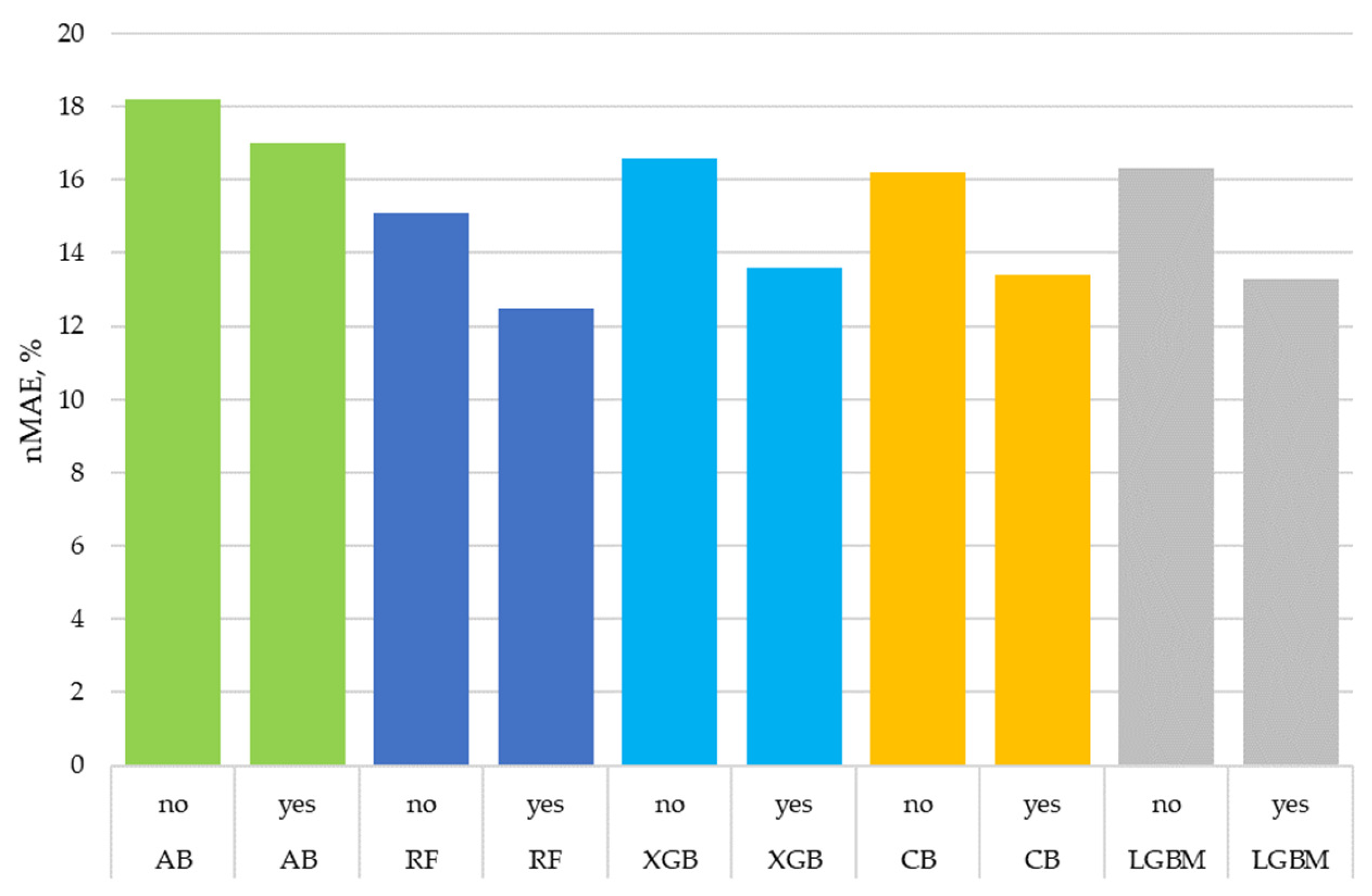
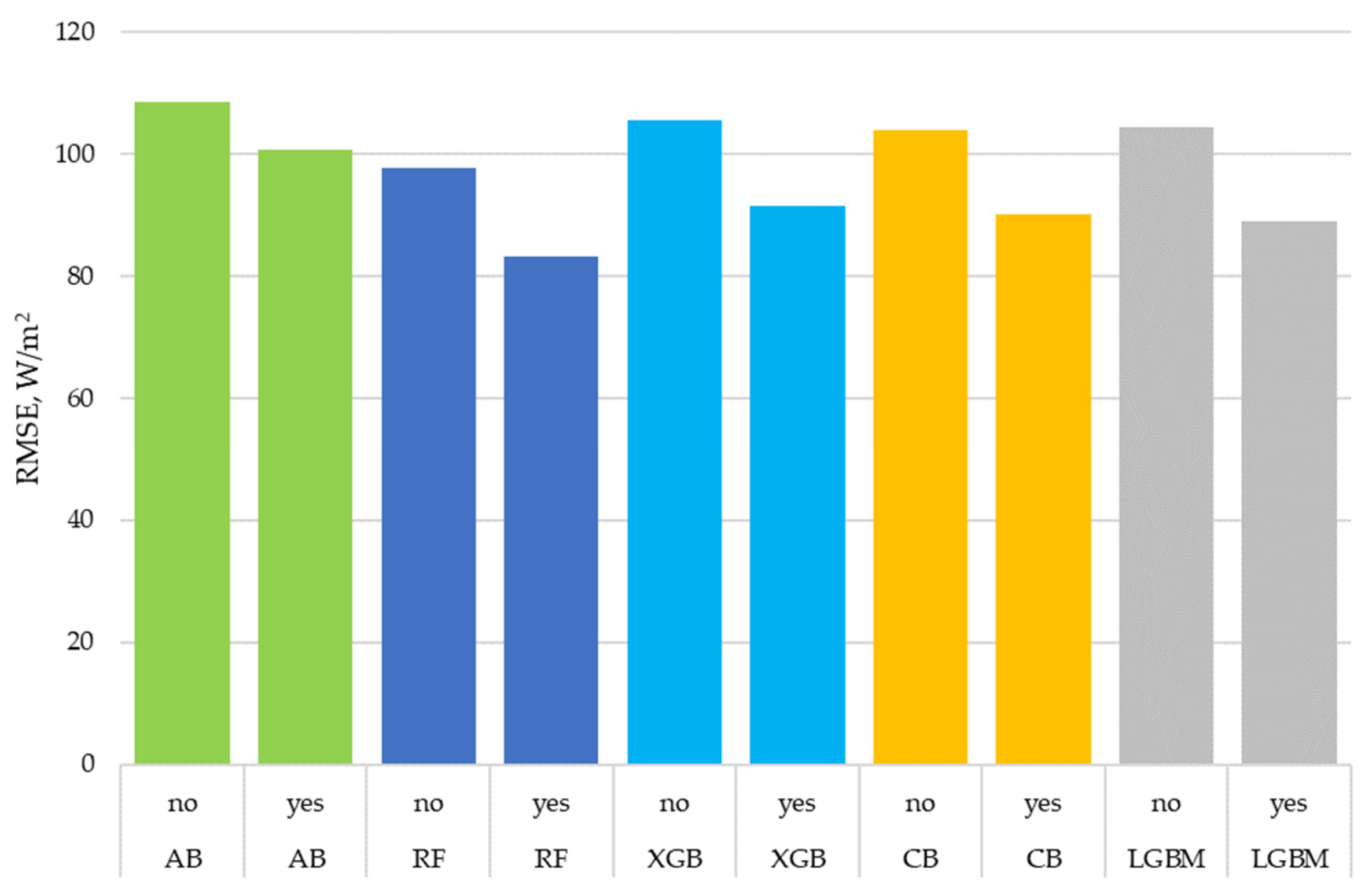
• The use of detailed cloud descriptions performed by the proposed algorithm significantly increased the accuracy of all ensemble models; the achieved averaged improvements were:
  • MAE by 15%;
  • nMAE by 15%;
  • RMSE by 12.7%;
  • R² by 5%.
• It should be noted that the overall cloud level as a percentage of the sky covered by clouds was used in all experiments. Thus, the difference in accuracy was ensured by the proposed algorithm for processing text descriptions of cloudiness in natural language.
• The decrease in accuracy for the kNN when using cloud descriptions may have been due to the fact that the kNN is less suitable for working with binary features.
• The best accuracy was obtained with the random forest algorithm; the CatBoost and LightGBM algorithms gave accuracies close to it.
• The resulting accuracy of random forest—R² = 0.91, nMAE = 12.5%—for the 3-h-ahead forecast of solar irradiance at tilted plane at the Earth’s surface corresponds to the state-of-the-art accuracy when taking into account differences in meteorological conditions between different territories.

Figure 7 and Figure 8 show two days from the testing dataset with a comparison of actual values and predicted values. A description of cloudiness, compared with using only the percentage of the sky covered by clouds, allows for error correction in both directions. With a high percentage of the sky covered, the clouds may not be dense and/or high, and vice versa, as with a low level of cloud cover, they may be dense and low.

3.2. The Interpretation Examples

For the RF (the model gave the smallest forecast error), the SHAP algorithm described above was applied, and visual interpretations of the forecasts were constructed. The first eight most important features are shown during visualisation. One interpretation explains the results of one model run to produce one forecast value of solar irradiance 3 h ahead.

In this case, the features associated with the position of the Sun and the intensity of solar irradiance at the top of the atmosphere (day, hour and irradiance at the atmosphere boundary) were combined during interpretation, since they are determined by date and time and have a general meaning for a user.

Figure 9, Figure 10, Figure 11, Figure 12, Figure 13 and Figure 14 present the SHAP visualisation of the model forecasts for different days. Each horizontal bar shows the significance of a correspondence feature. A positive value indicates that the feature leads to an increase in the forecast relative to the average target value; a negative value indicates the opposite. The larger the absolute value of the feature’s bar, the stronger the feature’s significance on the result (forecast).

Examples of forecasts interpretation using the SHAP visualisation approach:

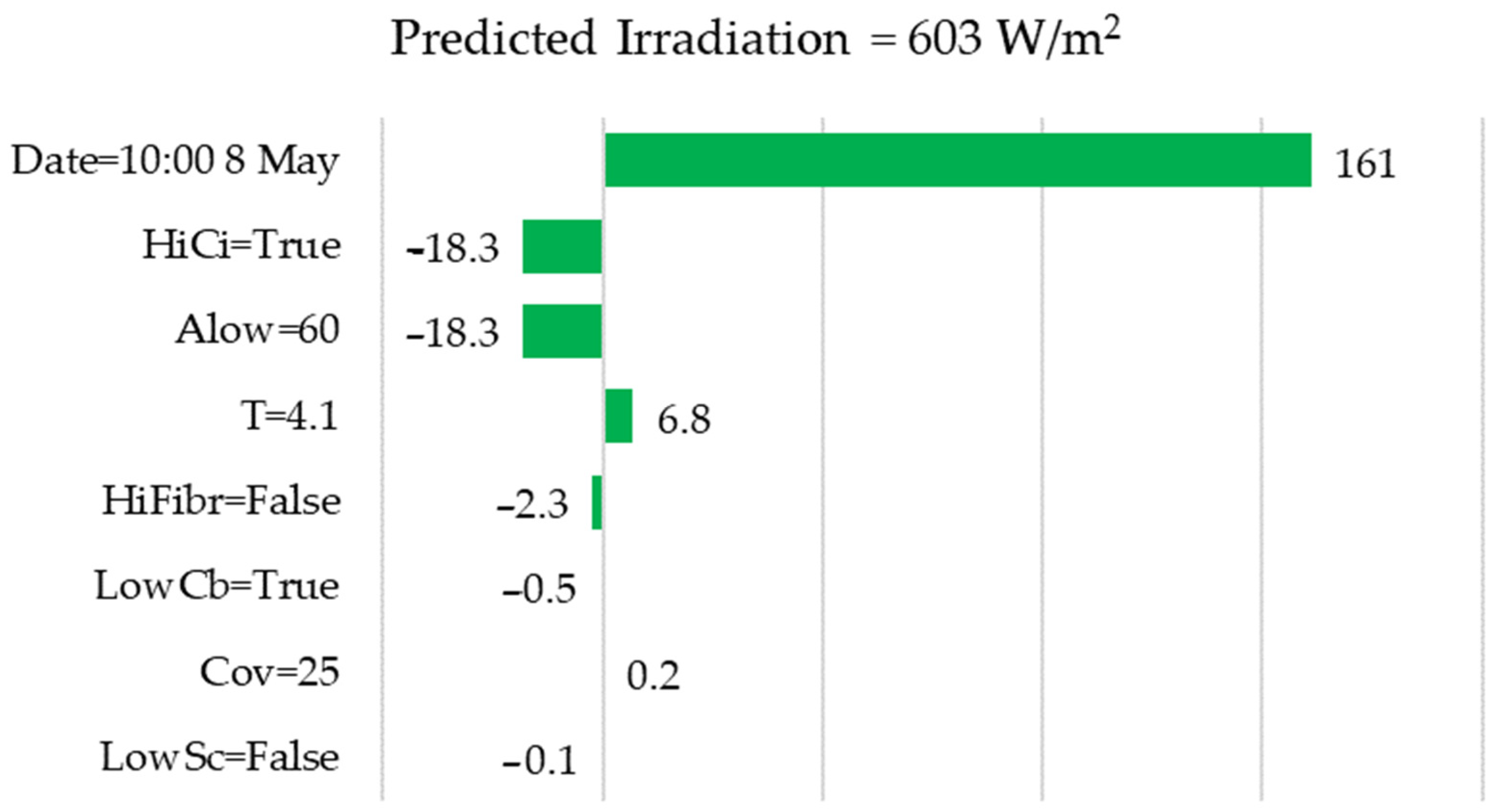
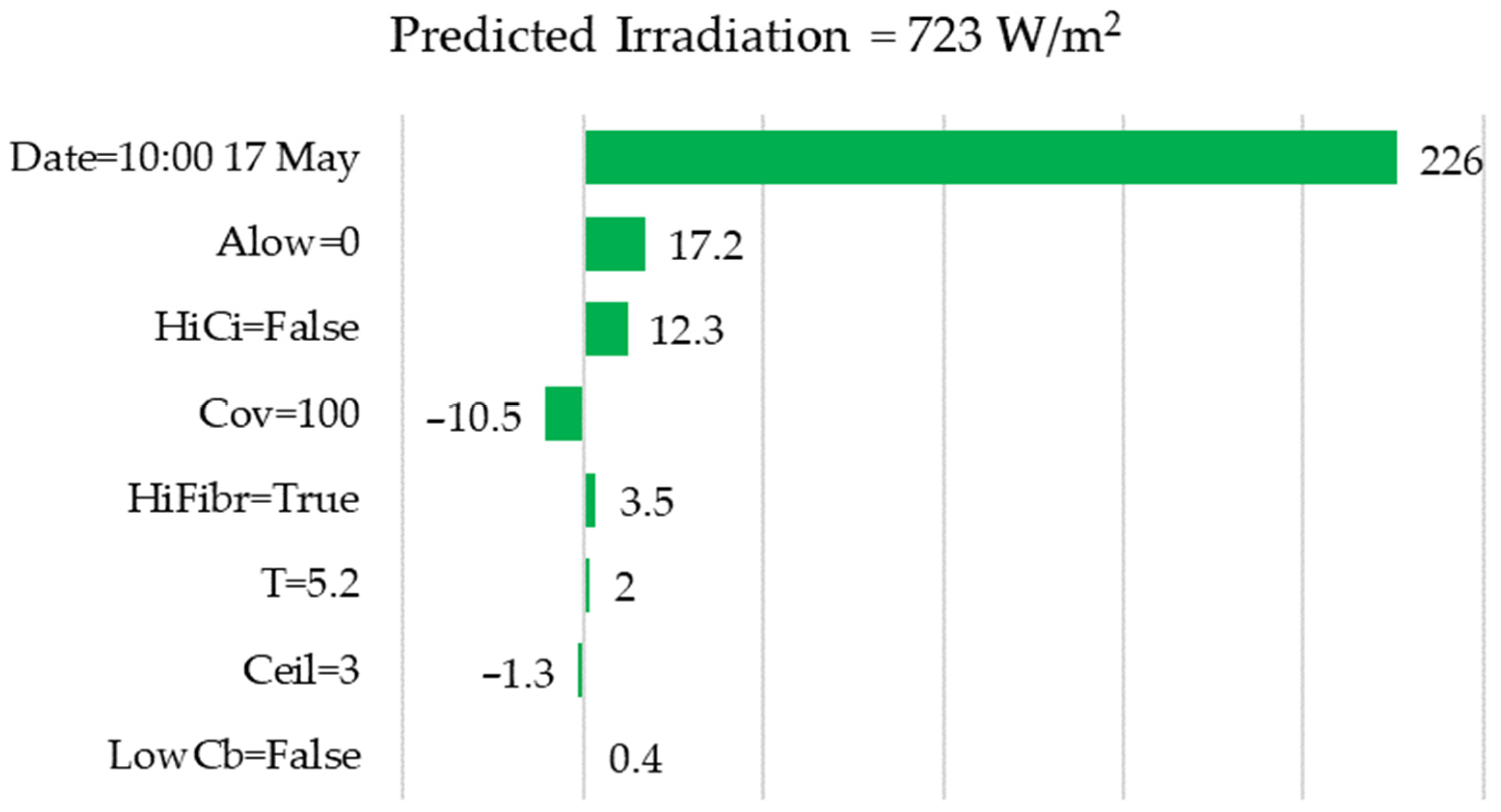
• Figure 9 shows that the model took into account the average percentage of low-level clouds (ALow = 60%) to reduce the forecast value, which is logical, since low-level clouds have a greater impact on the scattering of solar radiation. Also, the model took into account the absence of high cirrus clouds (HiCi = False) to improve the forecast, which is also logical.
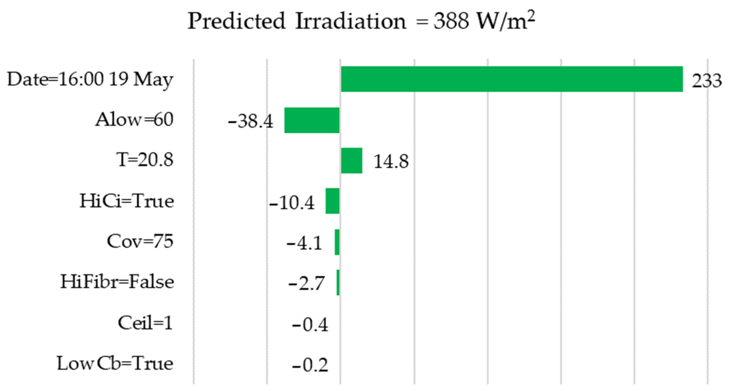
• For the following day and the same hour of the day, the forecast was slightly lower; from Figure 10, it is immediately clear that the reason was the presence of high cirrus clouds (HiCi = True).
• Figure 11 shows an example of another close day and the same hour of day, and the model forecast was significantly higher than for the example in Figure 9 and Figure 10. The model result is explained by the absence of low and medium clouds (ALow = 0%).

From a comparison of Figure 9, Figure 10 and Figure 11, we can conclude that the interpretation algorithm makes it possible for user to quickly understand why forecasts are so different for coinciding hours and close days of the year. Without interpretation of the results, the user would not be able to evaluate the logic of the model.

Our analysis of the interpretations obtained allows us to note that the feature often used in other studies to take into account cloudiness—the percentage of cloud coverage of the sky (Cov)—did not have much influence in the presence of features that describe cloudiness in more detail. For example, as seen in Figure 12, at 100% sky cover, the absence of low clouds and high cirrus made it possible for the model to improve the forecast despite cloudy weather.

Although experiments have shown that of all the binary features that describe cloud types, the presence of high cirrus clouds (HiCi) has a significant influence, other features also contribute and reduce the average forecast error. Examples are shown in Figure 13 and Figure 14, which demonstrate that the presence of Fractonimbus clouds (HiFbrn) had noticeable effects on the forecast.

Interpretations of forecasts allow one to not only explain an individual forecast during operation but also check the logic of the model at the stages of its validation and testing. The first use case is for the user, and the second one is for the developer.

In addition, the visualisation method used makes it possible to identify errors in the source data during operation of the intelligent information system. If data from the weather provider are lost, the user will see incorrect values in the visualisation dashboard. For example, the user may notice that the weather is cloudy in reality but the system generates a forecast in which all features of cloudiness have the values of 0 and False.

Table 8. The paper contributions versus others.

Paper	The Best Models	Cloud Data Usage	Forecast Explanation
[5,16,20]	MLP	No	No
[8]	LSTM	Clear sky index	No
[11,16,19,34,35]	DT ensemble	No	No
[12,33]	DT ensemble	Total cloud cover	No
[13,18,36,37,38]	LSTM	No	No
[15]	LSTM	Cloud type (as a single feature) and total cloud cover	No
[17,23]	MLP	Total cloud cover	No
[21]	ENN	No	No
[22]	SVR, ELM	No	No
[30]	LSTM	Total cloud cover	SHAP algorithm
[39]	MLP	No	Direct explainable neural network provides general dependencies, but not explanation for each individual forecast
This research	DT ensembles	The new algorithm to process cloud observations in natural language is proposed	The new modified SHAP algorithm was proposed for explanation of SPP generation forecasts

presents a comparison of the main contributions of the paper versus those already reported. The comparison includes only studies with machine learning methods.

4. Conclusions

The study proves that the accuracy of short-term solar irradiance forecasting and, therefore, that SPP generation can be improved by using detailed cloud description. To create a machine learning model, it is necessary to use meteorological retrospective data in which cloud descriptions are often given in a format close to natural language. Therefore, this paper proposed an algorithm for processing such data based on stemming and converting them into categorical and binary features.

Experiments were carried out on meteorological data and measurements of solar irradiance taken from a real solar power plant. It was determined that the proposed algorithm improved forecasting accuracy by 5–15%, depending on the quality metric used and the machine learning model. In particular, for the random forest, which showed the best results, the MAE decreased from 71 to 59 W/m² and R² increased from 0.87 to 0.91. The overall cloud level, as a percentage of the sky covered by clouds, was found to contribute less to the resulting forecasts than a set of features that describe cloudiness in detail. Taking into account differences in meteorological conditions between different territories, the resulting accuracy for the 3-h-ahead forecast corresponds to the state-of-the-art level.

The disadvantage of increasing the number of features is that the model becomes less transparent for users and developers. To overcome this shortcoming, the modified Shapley additive explanations method was proposed and applied. With this modification, features that have a meaning close to the user are aggregated and their weights are summed up. Examples were given to show how the visualisation of this method allows us to understand what a particular model forecast is based on. Such interpretive tools can increase specialists’ confidence in the intelligent information systems in the power industry.

The main contributions of the work comparing with already reported are the follows:

• Previous studies devoted to solar irradiation or SPP generation forecasting have used only total cloud cover or cloud data extracted from satellite images. This paper proposes to use types of clouds and other features that can be identified from cloud observations in natural language. It was experimentally proven that the use of various features describing cloudiness increases SPP generation forecasting.
• A new modification of the SHAP interpretation algorithm was proposed. For the first time, it was shown in detail how the SHAP algorithm can be used to explain obtained SPP generation forecasts.

In the course of further research, it is planned to conduct experiments on other objects, as well as develop a generative language model that, based on the results of the SHAP algorithm, will write a textual explanation of the models’ output.

References

1. Leon, L.F.; Martinez, M.; Ontiveros, L.J.; Mercado, P.E. Devices and control strategies for voltage regulation under influence of photovoltaic distributed generation. A review. IEEE Lat. Am. Trans. 2022, 20, 731–745. [Google Scholar] [CrossRef]
2. Ghulomzoda, A.; Safaraliev, M.; Matrenin, P.; Beryozkina, S.; Zicmane, I.; Gubin, P.; Gulyamov, K.; Saidov, N. A Novel Approach of Synchronization of Microgrid with a Power System of Limited Capacity. Sustainability 2021, 13, 13975. [Google Scholar] [CrossRef]
3. Bramm, A.M.; Eroshenko, S.A.; Khalyasmaa, A.I.; Matrenin, P.V. Grey Wolf Optimizer for RES Capacity Factor Maximization at the Placement Planning Stage. Mathematics 2023, 11, 2545. [Google Scholar] [CrossRef]
4. Prema, V.; Bhaskar, M.S.; Almakhles, D.; Gowtham, N.; Rao, K.U. Critical Review of Data, Models and Performance Metrics for Wind and Solar Power Forecast. IEEE Access 2022, 10, 667–688. [Google Scholar] [CrossRef]
5. Matrenin, P.; Manusov, V.; Nazarov, M.; Safaraliev, M.; Kokin, S.; Zicmane, I.; Beryozkina, S. Short-Term Solar Insolation Forecasting in Isolated Hybrid Power Systems Using Neural Networks. Inventions 2023, 8, 106. [Google Scholar] [CrossRef]
6. Raza, M.Q.; Nadarajah, M.; Ekanayake, C. On recent advances in PV output power forecast. Sol. Energy 2016, 136, 125–144. [Google Scholar] [CrossRef]
7. Gandoman, F.H.; Abdel, A.; Shady, H.E.; Omar, N.; Ahmadi, A.; Alenezi, F.Q. Short-term solar power forecasting considering cloud coverage and ambient temperature variation effects. Renew. Energy 2018, 123, 793–805. [Google Scholar] [CrossRef]
8. Hoyos-Gómez, L.S.; Ruiz-Muñoz, J.F.; Ruiz-Mendoza, B.J. Short-term forecasting of global solar irradiance in tropical environments with incomplete data. Appl. Energy 2022, 307, 118192. [Google Scholar] [CrossRef]
9. Shadab, A.; Ahmad, S.; Said, S. Spatial forecasting of solar radiation using ARIMA model. Remote Sens. Appl. Soc. Environ. 2022, 20, 100427. [Google Scholar] [CrossRef]
10. Voyant, C.; Notton, G.; Kalogirou, S.; Nivet, M.L.; Paoli, C.; Motte, F.; Fouilloy, A. Machine learning methods for solar radiation forecasting: A review. Renew. Energy 2017, 17, 569–582. [Google Scholar] [CrossRef]
11. Solano, E.S.; Dehghanian, P.; Affonso, C.M. Solar Radiation Forecasting Using Machine Learning and Ensemble Feature Selection. Energies 2022, 15, 7049. [Google Scholar] [CrossRef]
12. Alam, M.S.; Al-Ismail, F.S.; Hossain, M.S.; Rahman, S.M. Ensemble Machine-Learning Models for Accurate Prediction of Solar Irradiation in Bangladesh. Processes 2023, 11, 908. [Google Scholar] [CrossRef]
13. Li, P.; Zhou, K.; Lu, X.; Yang, S. A hybrid deep learning model for short-term PV power forecasting. Appl. Energy 2020, 259, 114216. [Google Scholar] [CrossRef]
14. Kumari, P.; Toshniwal, D. Deep learning models for solar irradiance forecasting: A comprehensive review. J. Clean. Prod. 2021, 318, 128566. [Google Scholar] [CrossRef]
15. Kumari, P.; Toshniwal, D. Long short-term memory–convolutional neural network based deep hybrid approach for solar irradiance forecasting. Appl. Energy 2021, 295, 117061. [Google Scholar] [CrossRef]
16. Basaran, K.; Özçift, A.; Kılınç, D. A New Approach for Prediction of Solar Radiation with Using Ensemble Learning Algorithm. Arab. J. Sci. Eng. 2019, 44, 7159–7171. [Google Scholar] [CrossRef]
17. Banik, R.; Das, P.; Ray, S.; Biswas, A. An Improved ANN Model for Prediction of Solar Radiation Using Machine Learning Approach. In Applications of Internet of Things; Springer: Singapore, 2021; pp. 233–242. [Google Scholar]
18. De, V.; Teo, T.T.; Woo, W.L.; Logenthiran, T. Photovoltaic Power Forecasting using LSTM on Limited Dataset. In Proceedings of the 2018 IEEE Innovative Smart Grid Technologies—Asia (ISGT Asia), Singapore, 22–25 May 2018; pp. 710–715. [Google Scholar]
19. Alaraj, M.; Kumar, A.; Alsaidan, I.; Rizwan, M.; Jamil, M. Energy Production Forecasting from Solar Photovoltaic Plants Based on Meteorological Parameters for Qassim Region, Saudi Arabia. IEEE Access 2021, 9, 83241–83251. [Google Scholar] [CrossRef]
20. Mutavhatsindi, T.; Sigauk, C.; Mbuvha, R. Forecasting Hourly Global Horizontal Solar Irradiance in South Africa Using Machine Learning Models. IEEE Access 2020, 8, 198872–198885. [Google Scholar] [CrossRef]
21. Wu, Z.; Wang, B. An Ensemble Neural Network Based on Variational Mode Decomposition and an Improved Sparrow Search Algorithm for Wind and Solar Power Forecasting. IEEE Access 2021, 9, 166709–166719. [Google Scholar] [CrossRef]
22. Karabiber, A.; Alçin, O.F. Short Term PV Power Estimation by means of Extreme Learning Machine and Support Vector Machine. In Proceedings of the 2019 7th International Istanbul Smart Grids and Cities Congress and Fair (ICSG), Istanbul, Turkey, 25–26 April 2019. [Google Scholar]
23. Matrenin, P.V.; Khalyasmaa, A.I.; Gamaley, V.V.; Eroshenko, S.A.; Papkova, N.A.; Sekatski, D.A.; Potachits, Y.V. Improving of the Generation Accuracy Forecasting of Photovoltaic Plants Based on k-Means and k-Nearest Neighbors Algorithms. ENERGETIKA Proc. CIS High. Educ. Inst. Power Eng. Assoc. 2023, 66, 305–321. (In Russian) [Google Scholar] [CrossRef]
24. WMO. Guide to Instruments and Methods of Observation, 2018th ed.; WMO 8; World Meteorological Organization: Geneva, Switzerland, 2018; pp. 490–492. [Google Scholar]
25. Utrillas, M.P.; Marín, M.J.; Estellés, V.; Marcos, C.; Freile, M.D.; Gómez-Amo, J.L.; Martínez-Lozano, J.A. Comparison of Cloud Amounts Retrieved with Three Automatic Methods and Visual Observations. Atmosphere 2022, 13, 937. [Google Scholar] [CrossRef]
26. Ahmed, I.; Jeon, G.; Piccialli, F. From Artificial Intelligence to Explainable Artificial Intelligence in Industry 4.0: A Survey on What, How, and Where. IEEE Trans. Ind. Inform. 2022, 18, 5031–5042. [Google Scholar] [CrossRef]
27. Adadi, A.; Berrada, M. Peeking Inside the Black-Box: A Survey on Explainable Artificial Intelligence (XAI). IEEE Access 2018, 6, 52138–52160. [Google Scholar] [CrossRef]
28. Ribeiro, M.T.; Singh, S.; Guestrin, C. Why Should I Trust You? Explaining the Predictions of Any Classifier. 2016. Available online: https://arxiv.org/abs/1602 (accessed on 15 February 2024).
29. Lundberg, S.M.; Erion, G.G.; Lee, S.-I. Consistent Individualized Feature Attribution for Tree Ensembles. 2018. Available online: http://arxiv.org/abs/1802.03888(accessed on 15 February 2024).
30. Kuzlu, M.; Cali, U.; Sharma, V.; Güler, O. Gaining Insight into Solar Photovoltaic Power Generation Forecasting Utilizing Explainable Artificial Intelligence Tools. IEEE Access 2020, 8, 187814–187823. [Google Scholar] [CrossRef]
31. Gabderakhmanova, T.S.; Kiseleva, S.V.; Frid, S.E.; Tarasenko, A.B. Energy production estimation for Kosh-Agach grid-tie photovoltaic power plant for different photovoltaic module types. J. Phys. Conf. Ser. 2016, 774, 012140. [Google Scholar] [CrossRef]
32. Murel, J. Stemming Text Using the Porter Stemming Algorithm in Python. 2023. Available online: https://developer.ibm.com/tutorials/awb-stemming-text-porter-stemmer-algorithm-python/ (accessed on 10 January 2024).
33. Khalyasmaa, A.I.; Eroshenko, S.A.; Tashchilin, V.A.; Ramachandran, H.; Piepur Chakravarthi, T.; Butusov, D.N. Industry Experience of Developing Day-Ahead Photovoltaic Plant Forecasting System Based on Machine Learning. Remote Sens. 2020, 12, 3420. [Google Scholar] [CrossRef]
34. Solano, E.S.; Affonso, C.M. Solar Irradiation Forecasting Using Ensemble Voting Based on Machine Learning Algorithms. Sustainability 2023, 15, 7943. [Google Scholar] [CrossRef]
35. Sarp, S.; Kuzlu, M.; Cali, U.; Elma, O.; Guler, O. An Interpretable Solar Photovoltaic Power Generation Forecasting Approach Using an Explainable Artificial Intelligence Tool. In Proceedings of the 2021 IEEE Power & Energy Society Innovative Smart Grid Technologies Conference (ISGT), Washington, DC, USA, 16–18 February 2021. [Google Scholar]
36. Sansine, V.; Ortega, P.; Hissel, D.; Hopuare, M. Solar Irradiance Probabilistic Forecasting Using Machine Learning, Metaheuristic Models and Numerical Weather Predictions. Sustainability 2022, 14, 15260. [Google Scholar] [CrossRef]
37. Elsaraiti, M.; Merabet, A. Solar Power Forecasting Using Deep Learning Techniques. IEEE Access 2022, 10, 31692–31698. [Google Scholar] [CrossRef]
38. Lee, W.; Kim, K.; Park, J.; Kim, J.; Kim, Y. Forecasting Solar Power Using Long-Short Term Memory and Convolutional Neural Networks. IEEE Access 2018, 6, 73068–73080. [Google Scholar] [CrossRef]
39. Wang, H.; Cai, R.; Zhou, B.; Aziz, S.; Qin, B.; Voropai, N.; Gan, L.; Barakhtenko, E. Solar irradiance forecasting based on direct explainable neural network. Energy Convers. Manag. 2020, 225, 113487. [Google Scholar] [CrossRef]
Figure 1. Types of data in the considered dataset.
Algorithms 17 00150 g001
Figure 2. General pipeline of the forecasting algorithm with the output interpretation.
Algorithms 17 00150 g002
Figure 3. MAE of ensemble models on a testing dataset with and without cloud descriptions.
Algorithms 17 00150 g003
Figure 4. nMAE of ensemble models on a testing dataset with and without cloud descriptions.
Algorithms 17 00150 g004
Figure 5. RMSE of ensemble models on a testing dataset with and without cloud descriptions.
Algorithms 17 00150 g005
Figure 6. R2 of ensemble models on a testing dataset with and without cloud descriptions.
Algorithms 17 00150 g006
Figure 7. An example of a day from a testing dataset. At 7:00, the forecast is overestimated, and at 19:00, it is underestimated without using the cloud description (Predicted Cloud Cover line).
Algorithms 17 00150 g007
Figure 8. An example of a day from a testing dataset. At 13:00 without using the cloud description, the forecast is underestimated (Predicted Cloud Cover line).
Algorithms 17 00150 g008
Figure 9. Example of interpretation, 7 May, 10:00.
Algorithms 17 00150 g009
Figure 10. Example of interpretation, 8 May, 10:00.
Algorithms 17 00150 g010
Figure 11. Example of interpretation, 9 May, 10:00.
Algorithms 17 00150 g011
Figure 12. Example of interpretation, 17 May, 10:00.
Algorithms 17 00150 g012
Figure 13. Example of interpretation, 13 May, 16:00.
Algorithms 17 00150 g013
Figure 14. Example of interpretation, 19 May, 16:00.
Algorithms 17 00150 g014