Article

Multi-Objective BiLevel Optimization by Bayesian Optimization

Insight Centre for Data Analytics, School of Computer Science and Information Technology, University College Cork, T12 XF62 Cork, Ireland
*
Author to whom correspondence should be addressed.
Algorithms 2024, 17(4), 146; https://doi.org/10.3390/a17040146
Submission received: 29 February 2024 / Revised: 22 March 2024 / Accepted: 26 March 2024 / Published: 30 March 2024

Abstract

:
In a multi-objective optimization problem, a decision maker has more than one objective to optimize. In a bilevel optimization problem, there are the following two decision-makers in a hierarchy: a leader who makes the first decision and a follower who reacts, each aiming to optimize their own objective. Many real-world decision-making processes have various objectives to optimize at the same time while considering how the decision-makers affect each other. When both features are combined, we have a multi-objective bilevel optimization problem, which arises in manufacturing, logistics, environmental economics, defence applications and many other areas. Many exact and approximation-based techniques have been proposed, but because of the intrinsic nonconvexity and conflicting multiple objectives, their computational cost is high. We propose a hybrid algorithm based on batch Bayesian optimization to approximate the upper-level Pareto-optimal solution set. We also extend our approach to handle uncertainty in the leader’s objectives via a hypervolume improvement-based acquisition function. Experiments show that our algorithm is more efficient than other current methods while successfully approximating Pareto-fronts.

1. Introduction

Bilevel optimization is a specific class of optimization problems consisting of the following two levels: the upper (leader) and lower (follower) levels. The lower-level problem is a constraint of the upper-level problem. It appears in the early 1950s in the context of Stackelberg game theory [1]. Because of the increasing complexity and size of bilevel problems, there is increasing interest in designing efficient algorithms to solve them in recent years. Bilevel problems may have single or multiple objectives at either or both levels. In the case of multiple objectives at the lower-level, a set of good solutions exists for each upper-level variable x u . So the upper-level decision maker observes the lower-level decision maker’s decisions via the x u decision variable. There are several domains where multi-objective bilevel optimization is used to solve real-world problems, such as the manufacturing industry [2,3], environmental economics [4,5], logistics [6,7] and defence [8]. In some applications, a solution must be found in real time so computational efficiency is crucial. Military applications and global security are examples of areas in which time is crucial and a hierarchy exists at each stage of the decision-making process.
Hierarchical decision-making under uncertainty with noisy objectives becomes more interesting in a bilevel structure. The follower can observe the leader’s decisions, but the leader may have no idea how the follower is going to respond. Previously observed decisions are therefore important. Most studies in the multi-objective bilevel optimization literature focus on solving the optimization problem without addressing the impact of uncertainty. In practical problems, noise in the leader’s objectives might represent environmental uncertainty, for example, in a meta-learning regime [9] that can be mathematically formulated as bilevel programming [10]. As another example, a government might need to prevent terrorist attacks using information from unreliable sources. Yet another example occurs in computing optimal recovery policies for financial markets [11]. Bilevel optimization problems are computationally expensive to solve because of their nested structure, and they become even more complex when there are multiple objectives and uncertainty (possibly at both levels).
Standard Bayesian optimization (BO) is a sequential experimental design framework for efficient global optimization of expensive-to-evaluate black-box functions, and has also been applied successfully to standard bilevel problems [12,13]. Multi-objective Bayesian optimization (MOBO) combines a Bayesian surrogate model with an acquisition function specifically designed for multi-objective problems. Hypervolume-based acquisition functions seek to maximize the volume of an objective space dominated by Pareto-front solutions. Expected hypervolume improvement (EHVI) [14] is a natural extension of the expected improvement acquisition function to multi-objective optimization. Single-objective problems can be derived from multi-objective problems by scalarizing objectives, for example, in ParEGO [15], which maximizes the expected improvement using random augmented Chebyshev scalarizations. MOEA/E-EGO [16] extends ParEGO to a batch setting using multiple random scalarizations and a genetic algorithm to optimize them in parallel. In [17], another batch variant of ParEGO was proposed. Called qParEGO, it uses compositional Monte Carlo objectives and a sequential greedy candidate selection process.
In this work, we first focus on solving multi-objective bilevel problems with a Gaussian process (GP) and a batch Bayesian approach in a noise-free setting. Then we extend the approach to handle the uncertainty in the leader’s objectives. We treat upper-level multi-objective problems as black-box functions and optimize them using Bayesian batch optimization with a multi-output GP as a surrogate model. Batch Bayesian optimization aims to query multiple locations at once. The benefit of this approach is that it makes parallel evaluations possible. Parallel evaluations are a vital part of various kinds of practical applications such as product design in the food industry, which can be modelled as bilevel problems with multiple objectives [18]. One can only produce a relatively small batch of different products at one time. Product quality, especially for foods, is usually highly dependent on the processing time since production. It is usually best to evaluate a batch immediately. So the next batch of products should be designed based on the feedback so far.
Many approaches have been developed for solving multi-objective bilevel problems. A particle swarm optimization algorithm is used to compute optimistic and pessimistic solutions in [19], who also developed a differential evolution algorithm to compute the four extreme solutions in [20]. Ref. [21] develop a nested differential evolution-based algorithm for multi-objective bilevel problems (DBMA). However, the necessary number of function evaluations is high, due to the nature of evolutionary algorithms. Satisfactory solutions are computed using leader preferences in [22]. Ref. [23] propose a hybrid evolutionary algorithm (H-BLEMO) but again gigantic computational cost was a problem. Ref. [24] develop a hybrid particle swarm optimization algorithm. Ref. [25] use a multi-objective particle swarm optimization algorithm and efficiently computes lower-level solutions (OMOPSO-BL). More details can be found in [20] on optimistic multi-objective bilevel problems.
Much work has been performed in the Bayesian literature on batch selection, and many developed specialized acquisition functions for batch Bayesian optimization. Some, such as qEI [26], qKG [27] and local penalization [28] methods, search for optimal batch selection. We use tailored acquisition functions to optimize the design space for multi-objective problems with fewer expensive function calls. To the best of our knowledge, there is no previous work on a batch Bayesian optimization approach to multi-objective bilevel problems [29]. The closest work is that of [30], which uses multiple Gaussian models for multiple objectives to solve robot and behaviour co-design, but not with batch selection during Bayesian optimization with upper-level objective uncertainty or with hypervolume improvement.
The aim of this paper is to improve computational efficiency to solve multi-objective bilevel problems while using hypervolume improvement to approximate the leader’s Pareto-optimal solution set. We compare the proposed algorithm with some existing algorithms in terms of function evaluations and hypervolume improvement. Moreover, we show how batch selection affects performance in batch Bayesian optimization. We propose two hybrid algorithms with a multi-objective Bayesian optimization approach to solve noise-free and noisy multi-objective bilevel problems, using two different acquisition optimizers specifically designed for multi-objective optimization. We use a non-dominated sorting genetic algorithm (NSGA-II) [31] to solve the lower-level multi-objective problems, with a crossover operator to decrease lower-level function evaluations. Using Bayesian batch optimization via a multi-output GP surrogate model in a multi-objective bilevel setting allows us to measure and handle uncertainties in the multi-objective upper-level design space. Selecting multiple points rather than one point at a time makes the optimization process more efficient. Moreover, the multi-output GP allows us to work with several kernels that worked well in the literature while optimizing the multi-objective upper-level design space.
The contribution of this work is threefold. First, we present two hybrid algorithms for solving multi-objective bilevel problems with noise-free settings, which is an extension of the workshop paper [32], and a noisy setting is added using Bayesian batch optimization. Second, batch Bayesian optimization allows us to use batch selection during optimization rather than just once per iteration. It provides information on how batch selection affects the whole bilevel optimization process at both levels. Third, we use the qNEHVI acquisition function and consider hypervolume improvement for solving the following q-batch decision points at the upper-level. This provides an approximation to the Pareto-optimal solutions with less expensive function evaluations.

2. Preliminaries

BO is a method to optimize expensive-to-evaluate black-box functions. It uses a probabilistic surrogate model, typically a GP [33] p ( f | D ) to model the objective function f based on previously observed data points D = { ( x 1 , y 1 ) , , ( x n , y n ) } . GPs are models that are specified by a mean function μ ( x ; { x n , y n } , θ ) : R d R and predictive variance function σ ( x ; { x n , y n } , θ ) : R d × R d R . A surrogate model p ( f | D ) is assisted by an acquisition function α : X R . We represent acquisition functions depending on the previous observations as α ( x ; { x n , y n } , θ ) , where θ is Gaussian parameters such as a kernel for the model. Because the objective function is expensive-to-evaluate and the surrogate-based acquisition function is not, it can be optimized more easily than the true function to yield x n e w . The acquisition function selects the point x n e w that maximizes the acquisition function x n e w = a r g m a x x X α ( x ) . It then evaluates the objective function y n e w = f ( x n e w ) and updates the data set with new observations D D ( x n e w , y n e w ) . In the GP, μ ( x ) can be viewed as the prediction of the function value, and  σ ( x ) is a measure of the uncertainty of the prediction.
Multi-objective BO tackles the problem of optimizing a vector-valued objective f ( x ) : R d R d with f ( x ) = ( f 1 ( x ) , , f d ( x ) ) for a vector-valued decision variable x R d . Because of the nature of multi-objective black-box problems, we assume that there is no known analytical expression. Multi-objective optimization problems generally do not have a single best solution, so we must find a solution set instead of a single solution; thus, the set of Pareto-optimal solutions. We say that f ( x ) dominates another solution f ( x ) if f ( i ) ( x ) f ( i ) ( x ) for all i = 1 , 2 , , M and there exists i { 1 , 2 , , M } such that f i ( x ) f i ( x ) . So we can express the Pareto-optimal solution set by P * = { f ( x ) s.t. x X : f ( x ) f ( x ) } and X * = { x X s.t. f ( x ) P * } . After obtaining the Pareto solution set, which is called the Pareto-front, the decision maker can make decisions using the trade-off between objectives, or any known preferences. In general, multi-objective optimization algorithms try to find a set of distributed solutions that approximate the Pareto-front.
Hypervolume improvement (HVI) is often used as a measure of improvement in multi-objective problems [34]. HVI is the volume that is dominated by the new point in the outcome space. It is generally nonrectangular and it can be computed efficiently by partitioning the non-dominated space into separate hyper-rectangles. This makes it a good candidate for seeking improvement in the outcome search space for the Pareto-optimal front. Figure 1 illustrates the hypervolume improvement in a 2 dimensional setting. The red area in the left graph represents the dominated solutions while the white area represents non-dominated solutions, and the green area in the middle graph represents the hypervolume improvement after the first point selection. The right graph illustrates the HVI in the q = 2 setting where q represents that batch selection in batch Bayesian optimization. Several methods have been proposed. EHVI is an updated version of expected improvement (EI) to HVI and determined by J ( x ) = E p ( f ( x ) | D n ) [ H V I ( f ( x ) ) ] . Previous work has considered unconstrained sequential optimization with ParEGO [15]. ParEGO is often optimized with gradient-free methods. qParEGO supports parallel and constrained optimization [17], and exact gradients are computed via auto-differentiation for acquisition optimization. This approach enables the use of sequential greedy optimization of q candidates with proper integration over the posterior at the pending points.
Multi-objective bilevel optimization problems have two levels of multi-objective optimization, such that a feasible solution to the upper-level problem must be a member of the Pareto-optimal set of lower-level optimization problems. Each level has its own variables, objectives and constraints. For the given upper-level vector x u the evaluation of the upper-level function is valid only if the x l is an optimum of the lower-level problem. A general multi-objective bilevel optimization problem can be described as follows:
minimize x u X u , x l X l { F 1 ( x u , x l ) , . . . , F M u ( x u , x l ) } subject to x l argmin x l { f 1 ( x u , x l ) , . . . , f M l ( x u , x l ) ; g j ( x u , x l ) 0 , j = 1 , 2 , , J } G k ( x u , x l ) 0 , k = 1 , 2 , , K .
In Equation (1) the upper-level objective functions are F i ( x u , x l ) , i = 1 , 2 , , M u and the lower-level objective functions are f i ( x u , x l ) , i = 1 , 2 , , M l , where x u X u and x l X l . G k ( x u , x l ) and g j ( x u , x l ) represent upper- and lower-level constraints, respectively. j and K values represent the number of constraints at the upper- and lower-level. The lower-level optimization problem is optimized with respect to x l considering x u as a fixed parameter.

3. Methodology

In this work, we solve a multi-objective upper-level problem with both noise-free and noisy settings by treating it as a black box. We solve a vector-valued upper-level problem, F ( x u , x l ) : R d × R v R M u , where d and v are number of upper-level and lower-level decision variable dimensions.
We assume that we have the upper-level multi-objective problem and use GP to model the objective functions F = { F 1 ( x u , x l ) , . . . , F M u ( x u , x l ) } where M u is the number of upper-level objective. Let us assume that we have the observed upper-level and lower-level decisions and upper-level objective values, D = { ( x u 1 , x l 1 , F ( x u 1 , x l 1 ) ) , , ( x u n , x l n , F ( x u n , x l n ) ) } , where n is the number of observations. The GP model is constructed with mean function and predictive variance function as follows, respectively:
μ ( x ; { x u n , x l n , F ( x u n , x l n } , θ ) σ ( x ; { x u n , x l n , F ( x u n , x l n } , θ )
where θ is the model parameters. The acquisition function selects the next upper-level decision by x u * = arg max x X α ( x ) . Then we evaluate the lower-level optimization and, after finding the optimum lower-level decision x l * regarding the upper-level decision, we update the data set with new observations D D ( x u * , x l * , F ( x u * , x l * ) ) . As in the GP, μ ( · ) can be viewed as the prediction of the function value and σ ( · ) is a measure of the uncertainty of the prediction.

3.1. Noise-Free Setting

An acquisition function for multi-objective Bayesian optimization (MOBO) is expected hypervolume improvement. Maximizing hypervolume (HV) is a procedure for finding the maximum coverage with Pareto-fronts [35]. We use the q-expected hypervolume improvement acquisition function (qEHVI) for a MOBO procedure at the upper-level. qEHVI computes the exact gradient of the Monte Carlo estimator using auto-differentiation, allowing it to employ efficient and effective gradient-based optimization methods. More details about the qEHVI can be found in [17]. Another acquisition optimizer we use is an extended version of a hybrid algorithm with on-line landscape approximation for expensive multi-objective optimization problems (ParEGO) [15]. It is extended to the constrained setting by weighting the expected improvement by the probability of feasibility, which is called qParEGO [36]. qParEGO uses a Monte Carlo-based expected improvement acquisition function, where the objectives are modelled independently and the augmented Chebyshev scalarization [15] is applied to the posterior samples as a composite objective. More details can be found in [17].
The proposed algorithm for a noise-free setting is a hybrid method for solving multi-objective bilevel optimization problems. Briefly, it works as follows: a population of the size of N u initial decisions, x u , is randomly selected from upper-level decision set X u . We used Sobol sampling for the initial random selection. For each upper-level decision, the lower-level problem is optimized using a non-dominating sorting genetic algorithm with population size N l . For a given x u , a Pareto-optimal solution set is obtained by the NSGA-II algorithm. Lower-level decision values are selected randomly from the Pareto-front obtained by the NSGA-II algorithm. We decided to use the random selection from the Pareto-optimal solution set following the work [37]. The solution set obtained after lower-level optimization iteration ( x u , x l * ) is used to find upper-level fitnesses F i ( x u , x l * ) for i = 1 , 2 , , M u . We train the GP model with the data set ( x u , y i ) where y i = F i ( x u , x l * ) . We use batch Bayesian optimization to choose the next candidates with the n-batch, which declares the number of the batch. In each Bayesian optimization iteration, the qEHVI and qParEGO acquisition optimizers suggest n-batch (q) candidates.
The lower-level optimization process is repeated for each candidate of the upper-level batch decision candidate x u . It is important to note that dealing with constraints is the most challenging aspect of bilevel problems. There are various approaches developed over the years, such as optimistic and pessimistic approaches regarding lower-level decision-making strategies; please see [38] for more details. While in the optimistic approach, the lower-level decision maker deals with the constraints and makes decisions considering the most favourable decision for the upper-level decision maker, the pessimistic approach assumes the least favourable decision for the upper-level. In this work, we considered the optimistic multi-objective bilevel problems and dealt with the constraints regarding the best interest of the leader. To avoid upper-level constraint violation, we made the random selection from lower-level Pareto-front considering the upper-level constraints. The algorithm runs for 50 iterations for the whole multi-objective bilevel optimization process. The details of the algorithm can be found in Algorithm 1.  
Algorithm 1: Upper-level Optimization
Inputs: F u ( x u , x l ) : x u X u , x l X l ,
Batch points per epoch q,
Number of iteration n,
Reference point
  1:
Initial decision data set D = { x u i , F u ( x u i , x l i * ) } i = 1 n with size of n ,
  2:
x l * : Initialize best lower-Level decisions as parameters from NSGA-2 Algorithm,
  3:
Initialize multi-objective Gaussian model with observations { x u , F u ( x u , x l * ) }
  4:
for i = 0 : N do
  5:
   Suggest new q-batch points by optimizing q-EHVI and qParEGO acquisition functions
  6:
   for j = 0 : q do
  7:
     For each upper-level decision x u , find optimal x l * by applying NSGA-2 algorithm
  8:
     Calculate fitness scores F u * and f u *
  9:
   end for
10:
   Update the data set D = ( x u i , F u ( x u i , x l i * ) ) i = 1 n
11:
end for
12:
Return Pareto-front F u * and corresponding optimum variables x u * , x l *

3.2. Noisy Setting

We consider a case that is crucial in practice, in which the leader must make decisions under uncertainty based on noisy observations F i = f ( x u i , x l i ) + ξ i , where ξ i N ( 0 , i ) and i is the noise covariance and x u , x l are upper and lower decision variables, respectively. We reformulate the leader’s objective with noisy observations as
minimize x u , x l { F 1 ( x u , x l ) + ξ 1 , . . . , F i ( x u , x l ) + ξ i }
where ξ i N ( 0 , i ) . Figure 2 represents the Pareto-front of noisy upper-level objective. We can observe that it is important to obtain a true Pareto-front with the uncertainty at upper level. The hypervolume indicator measures the volume of space between the non-dominated front and a reference point, which we assume is known by the upper-level decision-maker. The selection of reference points is tricky. In this work, it is chosen to be an extreme point of the Pareto-front, because reference points should be dominated by all Pareto-optimal solutions.
Hypervolume improvement of a set of points P is defined as H V I ( P | P , r ) = H V ( P P | r ) H V ( P | r ) , where P represents the Pareto-front and r the reference point. Given observations of the upper-level decision-making process, the GP surrogate model provides us with a posterior distribution over the upper-level function values for each observation. These values can be used to compute the expected hypervolume improvement acquisition function defined by
α e h v i ( x u | P ) = E [ H V I ( F u | P ) ] .
So the expected hypervolume improvement iterates over the posterior distribution, an approach that worked well in [39].
After n observations of the leader’s decisions and the follower’s response, the posterior distribution can be defined by the conditional probability p ( F ( x u n , x l n ) | D n ) of the leader’s objective values given decision variables ( x u n , x l n ) based on noisy observations D n = x u i , F i ( x u i , x l i ) , ( i ) i = 1 n . NEHVI is defined as
α NEHVI ( x u ) = α e h v i ( x u | P n ) p ( F | D n ) d F
where P n denotes the Pareto-optimal front optimal decision set over the leader’s objectives F n . The aim is to improve the efficiency of the optimization, and the handling of noise in the leader’s objective, by using the approach above and reformulating the bilevel multi-objective optimization problem. The algorithm details can be found in Algorithm 2.
Algorithm 2: Proposed Algorithm
Inputs: F u ( x u , x l ) : x u X u , x l X l ,
Batch points in each iteration Q,
The number of iterations for BO: N,
Reference point
  1:
x l : Find the best lower-level response as parameters with NSGA-II algorithm,
  2:
Initial decision data set with the objective noise
  3:
D = x u i , F u ( x u i , x l i ) , ( i ) i = 1 n with size of n,
  4:
Initialize the GP model with the observations and the objective noise
  5:
for i = 0 : N do
  6:
   Suggest new q-batch points by optimizing qNEHVI
  7:
   for j = 0 : q do
  8:
     For each upper-level decision x u , find optimal x l * by applying the NSGA-II
  9:
     Calculate fitness scores with noise F u ( x u , x l * ) + ξ
10:
   end for
11:
   Update the data set D with new observations
12:
end for
13:
Return Pareto-optimal front F u * and ( x u , x l * )

4. Experiments

We share the details of the experiments for the proposed approach in this section.

4.1. Noise-Free Experiments

First we consider noise-free settings.

4.1.1. Parameters

We use the Python programming language to implement the problems. BoTorch library [40] is used for the upper-level optimization problem. qEHVI and qParEgo acquisition functions for multi-objective optimization problems can be found in the library. SobolQMCNormalSampler is used for random sampling for starting the optimization. The main reason for choosing this sampling method is its popularity in the multi-objective Bayesian optimization literature. 2 ( d + 1 ) random upper-level decision points are selected, where d represents the dimensions of the problem for constructing the GP model as recommended in [14]. MaternKernel is used as it is the default selection. During acquisition optimization, we selected the number of starting points num _ restarts = 10 and raw _ samples = 512 as suggested in [14] for both the qEHVI and qParEGO acquisition functions. The multi-start optimization of the acquisition function is performed using LBFGS-B with exact gradients computed via auto-differentiation. Other parameters are set as default for Bayesian optimization to observe the performance. Lower-level optimization problems are solved using a genetic algorithm. For the implementation of the problems the PyMOO library [41] is selected. We use NSGA-II proposed in [31] with the following parameters. We selected pop_size = 50 to represent the population size, and the number of generations is set to 50. The main purpose of this selection is to make a fair comparison with other evolutionary methods, i.e., [25]. The real_random sampling method is used for sampling. After we obtained the Pareto-optimal solution set, we used a uniform random selection from the Pareto-optimal solution set. The algorithm is executed 10 times for each test function with different batch sizes.

4.1.2. Performance Measures

The multi-objective algorithms are assessed in terms of convergence to the Pareto-front and with respect to the diversity of the obtained solutions. In order to examine the proposed algorithm’s performance, we compare it with the OMOPSO-BL and H-BLEMO algorithms in terms of the hypervolume (HV) indicator and the inverted generational distance (IGD). We present our results in terms of function evaluations and compare them with DBMA and H-BLEMO. We use the same number of final sample sizes of the Pareto-optimal solution set to compare HV and IGD values with the other algorithms. HV measures the volume of the space between the non-dominated front obtained and a reference point. It is a common metric for comparing the performance of the obtained solutions with the true Pareto-front published for the problems. IGD calculates the sum of the distances from each point of the Pareto-front to the nearest point of the non-dominated set found by the algorithm. More details can be found for the metric in [42]. The IGD values of the DBMA algorithm are not reported [21] but we compare the results with the HV metric. Both HV and IGD measure the convergence and the spread of the obtained set of solutions.

4.1.3. Test Problems

We discuss the numerical experiments using the proposed algorithm on three different benchmark problems from [25], including quadratic unconstrained and linear constrained problems. Furthermore, we applied the proposed algorithm to the popular CEO problem from [24].

Problem 1

The problem has a total of three variables and is linear and constrained at both levels. The formulation of the problem is given in Table 1. Both upper- and lower-level optimization tasks have two objectives and the reference point for the problem is x r e f = ( 1 , 0 ) . The linear constraint in the upper-level optimization task does not allow the entire quarter circle to be feasible for some y. Thus, at most a couple of points from the quarter circle belong to the Pareto-optimal set of the overall problem. Reported Pareto-optimal solutions for the problem are in the third column of Table 1. Figure 3 on the left graph shows the Pareto-front solutions for Problem 1. Note that in this problem there exists more than one lower-level Pareto-optimal solution such as A in Figure 3. Therefore, in this problem finding the right Pareto-optimal lower-level solution is important for finding the correct bilevel decision set. Finding a solution like A makes the lower-level task useless, and this is the challenging part of the problem. Dashed lines represent the lower-level Pareto-fronts and B and C points as the two most Pareto-optimal solutions for the upper-level decision y = 0.9 .

Problem 2

The problem is quadratic and unconstrained at both levels. The formulation of the problem is given in Table 1. The reference point for the problem is x r e f = ( 1 , 0.5 ) . The upper-level problem has one variable and the lower-level has two variables. For a fixed x u the Pareto-optimal solutions of the lower-level optimization problem are given as { x l R | x u [ 0 , y ] , x l 1 = x l 2 = 0 }. For the upper-level problem, the Pareto-optimal solutions are reported in Table 1. As we can see in Figure 3 on the right, if an algorithm fails to find the true Pareto-optimal solutions of the lower-level problem and finds a solution, such as a point C, then it might dominate a true Pareto-optimal point such as point A. So finding true Pareto-optimal solutions is a difficult task in this problem.

Problem 3

We increase the dimension of the variable vector of Problem 2. The formulation of the problem is given in Table 1. The reference point for the problem is x r e f = ( 1 , 0.5 ) . The upper-level problem has one variable and the lower-level is scalable with K variables. For this work, K is set to 14 and the total number of variables is 15 in this problem. For a fixed x u , the Pareto-optimal solutions of the lower-level optimization problem are given as follows: { x l R K | x u [ 0 , y ] , x l i = 0 , for i = 2 , . . . , K }. For the upper-level problem, the Pareto-optimal solutions are formulated in Table 1.

Practical Case: CEO Problem

This case is taken from [24]. In a company, the CEO has the leader problem of optimizing net profit and the quality of products. The branch head has the follower problem of optimizing its own profit and worker satisfaction. According to the scenario above, the problem itself can be modelled as a multi-objective bilevel optimization problem. The deterministic version of the problem can be formulated as in Equation (6). Let the CEO’s decision variable be x u = ( x u 1 , x u 2 ) and the branch head’s decision variable be x l = ( x l 1 , x l 2 , x l 3 ) . The constraints model requirements, such as material, marking cost, labour cost and working hours.
Maximize ( x u , x l ) F ( x u , x l ) = x u 1 + 9 x u 2 + 10 x l 1 + x l 2 + 3 x l 3 9 x u 1 + 2 x u 2 + 2 x l 1 + 7 x l 2 + 4 x l 3 subject to x l argmax x l f ( x u , x l ) = 4 x u 1 + 6 x u 2 + 7 x l 1 + 4 x l 2 + 8 x l 3 6 x u 1 + 4 x u 2 + 8 x l 1 + 7 x l 2 + 4 x l 3 g 1 ( x u , x l ) = 3 x u 1 9 x u 2 9 x l 1 4 x l 2 61 0 g 2 ( x u , x l ) = 5 x u 1 + 9 x u 2 + 10 x l 1 x l 2 2 x l 3 924 0 g 3 ( x u , x l ) = 3 x u 1 + 3 x u 2 + 1 x l 2 5 x l 3 420 0 G 1 ( x u , x l ) = 3 x u 1 + 9 x u 2 + 9 x l 1 + 5 x l 2 + 3 x l 3 1039 G 2 ( x u , x l ) = 4 x u 1 2 x u 2 + 3 x l 1 3 x l 2 + 2 x l 3 94 ( x u 1 , x u 2 , x l 1 , x l 2 , x l 3 ) 0 .
While the CEO’s objective is to maximize the quality of the product and the net profit, the objective of the branch heads is to maximize worker satisfaction and branch profits.

4.1.4. Results and Observations

The statistics on function evaluations, hypervolume difference and inverted generational distance from Pareto-optimal are given in Table 2 and Table 3. The HV and IGD values are shared with the standard deviations of 21 runs. The standard deviations come from Bayesian optimization. It is clear from Table 2 that most computational effort is spent on the lower-level problem. Because of the nested structure of bilevel problems, the lower-level problem must be solved for every upper-level decision, so it is vital to improve upper-level performance for efficiency. We can observe that the upper-level function evaluations decreased significantly compared to DBMA and H-BLEMO. We could not compare the function evaluations with the OMOPSO-BL algorithm because of unavailability in [25]. We compare HV and the IGD values with DBMA, OMOPSO-BL and H-BLEMO algorithms in Table 3. It also includes the HV difference graph for different batch sizes. Although Bayesian optimization is not generally effective on high-dimensional problems, we nevertheless obtain results that are better than the other tested methods.

Problem 1

As shown in Table 2, function evaluations decreased significantly compared with DBMA and H-BLEMO algorithms for Problem 1. We observe that in Table 3, the hypervolume obtained by the proposed algorithm is slightly better than DBMA, H-BLEMO and OMOPSO-BL. We also show hypervolume values for different batch sizes of 2 , 4 , 8 . Because of a lack of observations for a batch size of q = 1 as we ran the algorithm for 50 iterations, the algorithm could not find better hypervolume values. The IGD values of observed values are not better than the OMOPSO-BL and H-BLEMO algorithms for this specific problem with batch sizes 2 , 4 , 8 , as we can observe from Table 3. We think that as the problem is linear, and because of limited iteration numbers, the algorithm could not get as close as the others. There were no reported IGD values for the DBMA algorithm on this comparison.

Problem 2

We can observe from Table 2 for Problem 2 that the proposed algorithm improves computational performance and decreases the function evaluations significantly compared to DBMA and H-BLEMO. The HV values are much better than DBMA, OMOPSO-BL and H-BLEMO algorithms as we can see from Table 3. Note that because of the unavailability of OMOPSO-BL and H-BLEMO experiment data, the results shown for these algorithms are taken from [25]. The IGD results in Table 3 show that the proposed algorithm approximates successfully to the Pareto-optimal solutions.

Problem 3

Table 2 shows that the proposed algorithm significantly decreases function evaluations during the optimization while approximating the Pareto-optimum solutions for Problem 3. We compare our results with DBMA and H-BLEMO algorithms, but not OMOPSO-BL because they did not share this information (as mentioned above). The HV value for batch size 1 is better than OMOPSO-BL but not H-BLEMO, as we can see in Table 3. However, the proposed algorithm reached better HV for batch size 8. IGD values are shown in Table 3 and we can observe that the approximation solution sets are not as close as the other algorithms. However, we think that considering the significant decrease in function evaluations, it shows good performance.

Practical Case: CEO Problem

For the CEO problem, they use a weighted sum method to obtain a single optimal solution x u = ( 146.2955 , 28.9394 ) and x l = ( 0 , 67.9318 , 0 ) in [24]. They use a hybrid particle swarm optimization algorithm with a crossover operator in [24]. Ref. [43] present Pareto-front solutions and extreme points using CMODE/D algorithm. We present the extreme points of our results in Table 4. The proposed algorithm can obtain the Pareto-front containing the single optimal solution obtained in [43]. We focused on the extreme points on the Paret-front solution set to make the comparison with the solutions in [43]. As we can observe, the obtained optimal solutions in Table 4 cover more broadly in terms of the objectives. We also share the optimal decisions for the leader and the follower for better comparison. The experiments use both qNEHVI and qParEGO and all batch sizes. Table 4 presents the best results obtained.

4.2. Noisy Experiments

The test problems are selected from the literature [44], to test scalability in terms of decision variable dimensionality. The results are compared with state-of-art evolutionary algorithms m-BLEAQ [45] and H-BLEMO [23]. The Pareto-optimal front is independent of the parameters. Furthermore, we use a real-world problem from the environmental economics literature, which considers a hierarchical decision-making problem between an authority and a gold mining company [46].

4.2.1. Performance Metrics

We compare our results in terms of upper-level function evaluations (FE) to determine the efficiency of the algorithm as Bayesian optimization aims to minimize the function evaluations while optimizing the expensive black-box functions. Hypervolume improvement [47] and inverted generational distance [42] are used to evaluate the success of approximation to Pareto-optimal fronts in terms of convergence and diversity. HV measures the volume of the space between the non-dominated front obtained and a reference point. IGD calculates the sum of the distances from each point of the true Pareto-optimal front to the nearest point of the non-dominated set found by the algorithm. Therefore, a smaller IGD value means approximated points are closer to the Pareto-optimal front of the problem.

4.2.2. Parameters

We fixed the number of Bayesian optimization iterations to N = 50 and repeated our experiments 21 times to obtain median results for making the comparison fair. We use the independent GP model with Matern52 kernel and fit the GP by maximizing the marginal log-likelihood. The method is initialized with 2 × ( d + 1 ) Sobol points where d represents the dimension of the problem to construct the initial GP model. All experiments are conducted using the BoTorch [40] library. We solved the follower’s problem with the popular NSGA-II [31] and chose the population size 100 and number of generations 200. We choose the follower’s decisions from the obtained Pareto-optimal front at random, as all solutions in the Pareto-optimal front are feasible.

4.2.3. Test Problems

Example 1

The first example is a bi-objective problem that is scalable in terms of the number of follower decision variables. The formulation of the problem is given in Table 5. We choose K = 14 and K = 19 , giving 15 and 20 follower variables, respectively, with 1 leader decision variable. We choose the reference point required to measure hypervolume improvement to be ( 1.0 , 0.5 ) . The Pareto-optimal decision sets for this specific bilevel decision-making problem can be found in [45].

Example 2

The second test problem is the modified test problem with 10 and 20 variable instances. The formulation of 264 the problem is given in Table 5. We choose the required reference point to be ( 1.1 , 1.1 ) . The Pareto-optimal front for a given leader is defined as a circle of radius ( 1 + r ) with center ( ( 1 + r ) , ( 1 + r ) ) . We choose K = 5 for our experiments, with parameters r = 0.1 , τ = 1 and α = 1 , following [45] so that our results can be compared with those for m-BLEAQ and H-BLEMO.

Example 3

The third test problem is the modified test problem with 10 and 20 variable instances. The formulation of 264 the problem is given in Table 5. We choose the required reference point ( 0.8 , 0.0 ) for measuring the hypervolume improvement during the optimization. Details on the Pareto-optimal solutions are given in [48].

Practical Case: Gold Mining in Kuusamo

The Kuusamo region is a popular tourist destination known for its natural beauty. There is a lot of interest in this region cause it contains a huge amount of gold deposits and is considered to be a “highly prospective Paleoproterozoic Kuusamo Schist Belt” [49]. The expected gold amount in the ore is around 4.9 g per ton according to an Australia-based gold mining company. Even though there is a big potential in terms of providing lots of jobs in the region and leading to a great amount of gold resources, there are concerns about harming the environment. The first of them is that mining operations may cause pollution of the river water in the region. This concerns environmentalists. Second, the ore in the region contains uranium and, if it is mined, it might harm the reputation of nearby tourist resorts. Another is the open pit mines around the area called Ruka, which will affect nearby skiing resorts and hiking routes and reduce tourist interest. The regulating authority, which is the government, acts as a leader, and the mining company is the follower, which reacts rationally to the decisions of the leader in order to maximize its own profit. The leader should find an optimal strategy assuming that he holds the necessary information about the follower. In the situation explained above, the government has a decision-making problem, which is whether to allow mining and to what extent.
In the problem above, the leader has two objectives while the follower has one. The first objective is the maximization of revenues coming from the project and the second objective is to minimize the environmental harm, which is a result of the mining. The mining company also aims to maximize its own profit. While the government is optimizing its own taxation strategy, it needs to model how the mining company reacts to any given tax structure. Therefore, the authority makes an environmental regulatory decision instead of solving the problem to optimality. Clearly, the objectives are conflicting, such as the fact that large profits may affect the environment by increasing the damage, which follows with a bad public image. The mathematical formulation of this hierarchical decision-making problem can be found in Table 6. More details can be found about the bilevel modelling of the problem in [45,46]. Figure 4 presents the Pareto-optimal frontier of the given problem for the government according to the formulation in Table 6. We can observe that increasing the tax revenue decreases the environmental damage.

4.2.4. Results of Test Problems
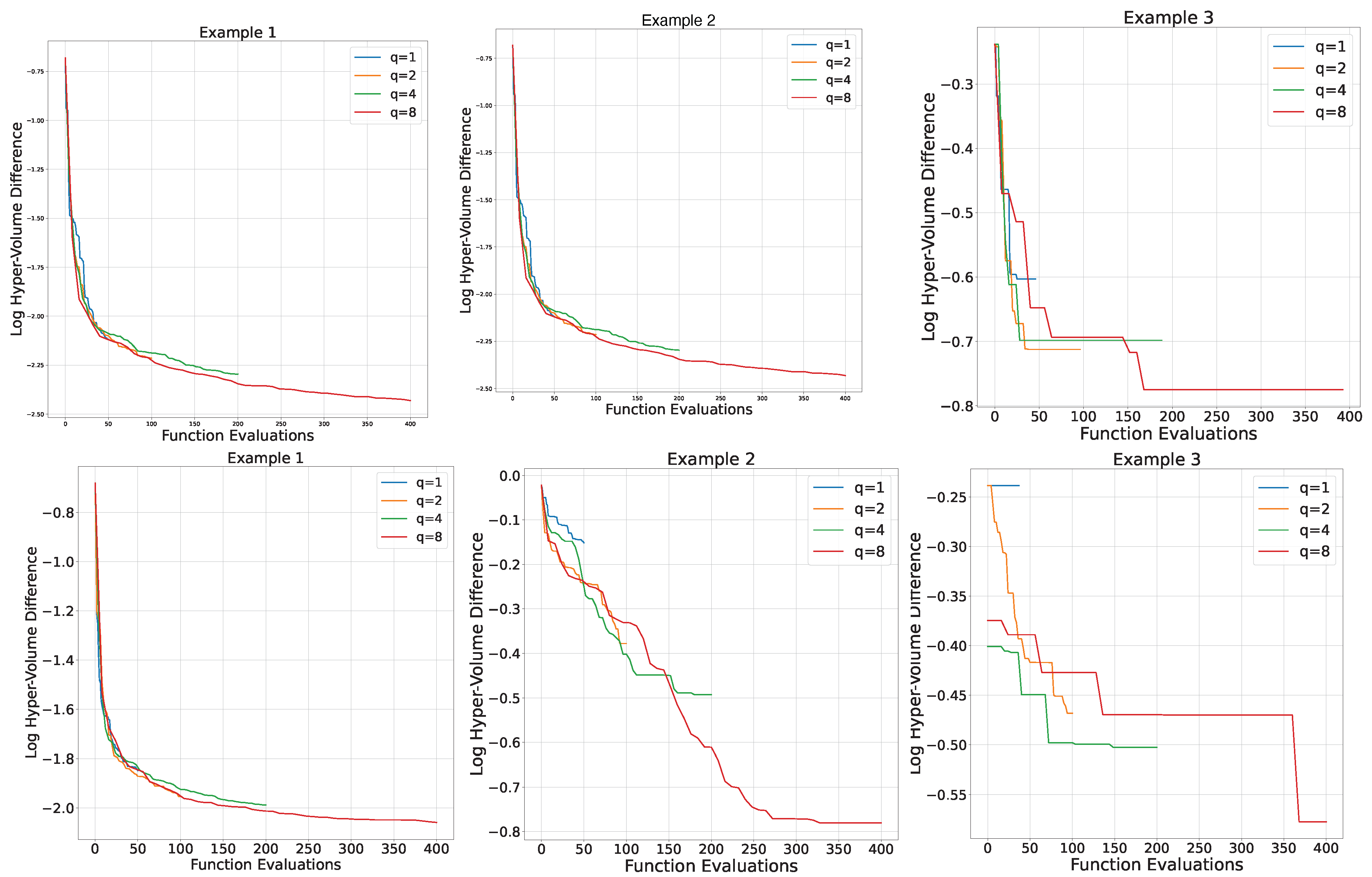
The performance of the proposed algorithm is compared with that of m-BLEAQ and H-BLEMO in Table 7, showing computational expense and convergence. The FE is calculated by N initial + ( N batch × N iter × N restarts ) for the leader problem, where N initial is the number of initial decisions for starting the algorithm, and N r e s t a r t s is the parameter for Gaussian process declaring the number of restarts to avoid becoming trapped in local optima. We choose it to be 2 × ( d + 1 ) , where d is the dimension of the decision variable. We run the experiment for different batch numbers q = 1 , q = 2 , q = 4 , q = 8 to test the effect on performance. The HV difference is shown in Figure 5 for 15 and 20 variables, and 10 variables for Examples 1 and 2, respectively. While increasing the batch size, decreasing the HV difference, as presented in Figure 1, shows the convergence of the proposed algorithm. Because of a lack of information in the reference paper, we could not obtain the FE results for Example 1 with 20 variables.

Example 1

We can see from Table 7 that the required upper-level FE is significantly lower, and the algorithm approximates successfully to the Pareto-optimal front while handling the uncertainty at the leader’s objective. For 15 variables, our proposed algorithm achieves 38 % improvement in terms of FE compared to m-BLEAQ and a ≈ 89 % compared to H-BLEMO. The IGD values in Table 7 for 15 and 20 variables show that it successfully approximates the Pareto-optimal front of the problem while handling the uncertainty of the leader’s objective for both. We show the HV difference between the Pareto-optimal front solutions and approximated decisions algorithm in Figure 5. Again we tried different batch sizes for the experiment, and it can be seen that a batch number of 8 is best for this specific example at both dimensions. We could not compare the 20-dimensional version of the problem with the selected algorithms because of a lack of information in [45].

Example 2

Table 7 shows that our proposed algorithm obtains the best IGD results compared to the other algorithms. In terms of FE, it significantly improves the state of the art, with an ≈ 81 % improvement for 10 variables and an ≈ 88 % improvement for 20 variables compared to m-BLEAQ. We also show the HV difference in Figure 5, and we can observe that, for this specific example, the batch number of 8 is the best selection for both 10 and 20 dimensional versions.

Example 3

Table 7 shows that our algorithm obtains the best IGD value compared to m-BLEAQ and H-BLEMO while improving efficiency in terms of FE: ≈ 84 % and ≈ 97 % with 10 variables, and ≈ 89 % and ≈ 98 % with 20 variables.
Figure 5 shows that a batch size q = 8 gives the best results. In summary, our proposed algorithm is successful on the selected test problems while handling noisy objectives with less computational cost. Noise in the leader’s objective makes the problem harder to solve but more realistic for modelling practical problems, because of real-world uncertainty. We show the proposed algorithm works well on these test benchmark problems.

Practical Case: Gold Mining in Kuusamo

In this section, we present the results obtained using the proposed algorithm on the analytical model of the problem proposed in Table 6. Figure 4 shows the Pareto-optimal front obtained using our approach. The plot gives the idea to the authority how to consider the trade-off between its own objectives. We used 50 iterations for upper-level optimization using a batch Bayesian approach with a batch size of 4. For lower-level optimization, the NSGA-II algorithm is implemented with the same parameters specified in Section 4.2.2. We can observe that with the proposed method, the obtained results are distributed around the true Pareto-optimal frontier and approximate to it successfully. We also run the experiments for the batch size q = 1 , q = 2 and q = 4 for testing if the algorithm converges to the Pareto-optimal front. The IGD value is 0.0494 for q = 1 , 0.0033 for q = 2 and 0.0021 for q = 4 . We can see from the decreasing IGD values that, as we increase the batch number, the selected points more closely approximate the true Pareto-optimal front. The increasing batch size provides us with parallel evaluations during upper-level optimization, which decreases the needed execution time. It is also important to handle environmental uncertainty, represented by ξ in Table 6, which may be an uncontrollable parameter, such as inflation, during the time period of taxation or unexpected environmental damage during the mining process. We can observe that the proposed method is successfully approximated even handling the uncertainty of objectives.
We believe that our proposed algorithm can be applied to several practical bilevel problems successfully applied in the machine learning community, such as image classification [50], deep learning [51], neural networks [52] and hyperparameter optimization [53].

5. Discussion

Compared with the evolutionary algorithms for the noise-free setting of the bilevel problem, approaching the upper-level problem as a black box obtains the Pareto-optimal front with much fewer function evaluations. For instance, when we look at Problem 2 in Table 2, the necessary function evaluation number decreased by almost % 64 for the upper-level, and % 91 for the lower-level problem compared with the DBMA method for the batch size of 4 setting of the proposed method. It implies that unnecessary evaluations can be significantly decreased by assuming we do not know the exact problem characteristics of upper-level decision-makers. Furthermore, the proposed algorithm can achieve better HV and IGD values for all theoretical problems compared to the rewarding solutions. In Problem 1, the HV value for Problem 1 is 0.3773 , while the closest one is DBMA with 0.3075 for the batch number of 8. Note that with the other batch numbers, even the sequential ( q = 1 ) setting reached better results than the evolutionary algorithms. When we look at the high-dimensional problem, the results for Problem 3 in Table 3 show that the proposed algorithm successfully approximated the Pareto-optimal front for the upper-level problem. We should note that the theoretical problems are relatively simple but, as we can see from the CEO problem, real-world problems can be modelled in this manner, and they can reflect the decision-making problems where there is no uncertainty.
In addition, the importance of uncertainty cannot be underestimated regarding real-world decision-making problems, especially given the hierarchy between decision-makers. Compared with the evolutionary algorithms, the proposed Bayesian optimization approach to uncertain upper-level problems approximates successfully to the true Pareto-optimal front. For instance, the final solution set of Examples 1, 2 and 3 with a smaller number of variables is well-distributed to the true Pareto-optimal front with much fewer function evaluations, please see Table 7. For the gold mining problem, the final obtained solution is distributed successfully as well, as we can see in Figure 4. The gold mining problem is relatively simple compared with the test problems and we can see that it can deal with both linear and quadratic problems.
Batch selection is also important for batch Bayesian optimization, and the experiments show that there is no single optimum batch number for all problems. For example, considering Problem 3 with q = 8 setting, the proposed algorithm approximated the true Pareto-optimal front with less function evaluation than the q = 4 setting while it is not the case on other problems. When we consider the collaboration of followers and leaders, it implies that the algorithm converges much faster than evolutionary algorithms when the problem dimension increases and collaboration of lower-level decisions increases, respectively.
In general, there is no single optimum batch number for solving upper-level problems during multi-objective Bayesian optimization, and the participation of lower-level decisions in upper-level problems should be considered. We can also conclude that either with or without uncertainty, the black-box approach performs better than existing exact and evolutionary approaches. Moreover, this development has the potential to explore more analyses of how problem characterization affects the surrogate model-based approaches, and to apply to many more real-world applications while leveraging the benefit of not necessarily knowing the specification of the mathematical model.

5.1. Limitations

Multi-objective bilevel problems are computationally expensive to evaluate. Even without uncertainty at the upper-level, there may be a lack of performance during the acquisition optimization process of the proposed algorithm. Furthermore, the Pareto-optimal solution set may not always provide the optimal solution for all objectives. Another limitation of the proposed algorithm is the lack of success of the Bayesian optimization with a high-dimensional search space. Even though there are some works in the literature on black-box optimization for high-dimensional data, this still limits the computational performance given the millions of variables. However, as we can see from Section 4.2.4, when approximating the Pareto-front in fairly high dimensions, the black-box approach improves performance compared with various existing methods.

6. Conclusions

Multi-objective bilevel optimization problems constitute one of the hardest classes of optimization models known, as they inherit the computational complexity of the hierarchical structure and optimization. We propose a hybrid algorithm, based on batch Bayesian optimization to reduce the computational cost of the problem.
Our contribution is three-fold in the literature of multi-objective bilevel optimization. First, we embed two specifically designed acquisition function optimizers for multi-objective problems based on hypervolume improvement and parallel evaluations during optimization to approximate the leader’s Pareto-front solutions. The proposed algorithm is explained in Section 4.1. Second, we discussed bilevel multi-objective optimization under upper-level uncertainty and presented another hybrid algorithm based on batch Bayesian optimization with noisy hypervolume improvement in Section 4.2. Moreover, we explore how batch size selection affects the optimization process for each of the proposed approaches. Third, we evaluate our proposed algorithm on six numerical and two real-world problems selected from the environmental economics literature, which is a decision-making problem between an authority and the followers, and compare our results with state-of-the-art algorithms. The results show that the proposed algorithm improves efficiency by significantly reducing computational cost. The proposed algorithm performed very competitively in terms of necessary function evaluation and convergence considering hypervolume improvement and IGD values.

Future Work

The preferences of decision are important when we consider the hierarchical decision-making processes. For instance, the follower’s decision from the Pareto-optimal front affects the leader’s problem and final solution set. In future work, we shall explore the decision-making from the Pareto-optimal front and how preference learning might affect the process. It would also be interesting to apply the proposed algorithm to the problems in the automated machine learning literature. For example, integrating the upper-level problem as a neural architecture search with considering multiple neural network models and lower-level problems to search the optimum hyperparameters for the candidate neural networks. As we mentioned with regard to the high-dimensional search space problem in Section 5.1, it might be interesting to explore how the proposed algorithm can be improved by using a high-dimensional Gaussian process [54] during the upper-level optimization. Moreover, we will look to gain some information by analyzing the relationship between the acquisition selection and the whole bilevel optimization results to observe how acquisition function selection affects the performance for obtaining the Pareto-optimal front at each iteration.

Author Contributions

Conceptualization, V.D.; methodology, V.D.; software, V.D.; validation, V.D. and S.P.; formal analysis, V.D.; investigation, V.D.; resources, V.D.; data curation, V.D.; writing—original draft preparation, V.D.; writing—review and editing, S.P.; visualization, V.D.; supervision, S.P.; funding acquisition, S.P. All authors have read and agreed to the published version of the manuscript.

Funding

This publication has emanated from research conducted with the financial support of Science Foundation Ireland under Grant number 12/RC/2289-P2 at Insight the SFI Research Centre for Data Analytics at UCC, which is co-funded under the European Regional Development Fund. For Open Access, the author has applied a CC BY public copyright licence to any Author Accepted Manuscript version arising from this submission.

Data Availability Statement

The original contributions presented in the study are included in the article, further inquiries can be directed to the corresponding authors.

Conflicts of Interest

The authors declare no conflicts of interest. The funders had no role in the design of the study; in the collection, analyses, or interpretation of data; in the writing of the manuscript; or in the decision to publish the results.

Abbreviations

The following abbreviations are used in this manuscript:
ParEGOParallel Efficient Global Optimization
MOEAMulti-Objective Evolutionary Algorithm
DBMADecomposition-Based Memetic Algorithm
H-BLEMOHybrid EMO-Cum-Local-Search Bilevel Programming Algorithm
OMOPSO-BLMulti-objective Optimization by Particle Swarm Optimization for Bilevel Problems
NSGA-IINon-Dominated Sorting Genetic Algorithm
CMODE/DCompetitive Mechanism-Based Multi-Objective Differential Evolution Algorithm
m-BLEAQMulti-Objective Bilevel Evolutionary Algorithm Based on Quadratic Approximations
MOBOMulti-objective Bilevel Optimization
EHVIExpected Hypervolume Improvement
NEHVINoisy Expected Hypervolume Improvement
IGDInverted Generational Distance
HVIHypervolume Improvement
HVHypervolume Improvement
GPGaussian Process
EIExpected Improvement
FEFunction Evaluation
BOBayesian Optimization
qEIq-Expected Improvement
qKGq-Knowledge Gradient

References

  1. Stackelberg, H.v. The Theory of the Market Economy; William Hodge: London, UK, 1952. [Google Scholar]
  2. Gupta, A.; Kelly, P.; Ehrgott, M.; Bickerton, S. Applying Bi-level Multi-Objective Evolutionary Algorithms for Optimizing Composites Manufacturing Processes. In Evolutionary Multi-Criterion Optimization; Purshouse, R.C., Fleming, P.J., Fonseca, C.M., Greco, S., Shaw, J., Eds.; Springer: Berlin/Heidelberg, Germany, 2013; pp. 615–627. [Google Scholar]
  3. Gupta, A.; Ong, Y.S.; Kelly, P.A.; Goh, C.K. Pareto rank learning for multi-objective bi-level optimization: A study in composites manufacturing. In Proceedings of the 2016 IEEE Congress on Evolutionary Computation (CEC), Vancouver, BC, Canada, 24–29 July 2016; pp. 1940–1947. [Google Scholar] [CrossRef]
  4. Barnhart, B.; Lu, Z.; Bostian, M.; Sinha, A.; Deb, K.; Kurkalova, L.; Jha, M.; Whittaker, G. Handling practicalities in agricultural policy optimization for water quality improvements. In Proceedings of the Genetic and Evolutionary Computation Conference, GECCO ’17, Berlin, Germany, 15–19 July 2017; pp. 1065–1072. [Google Scholar] [CrossRef]
  5. del Valle, A.; Wogrin, S.; Reneses, J. Multi-objective bi-level optimization model for the investment in gas infrastructures. Energy Strategy Rev. 2020, 30, 100492. [Google Scholar] [CrossRef]
  6. Gao, D.Y. Canonical Duality Theory and Algorithm for Solving Bilevel Knapsack Problems with Applications. IEEE Trans. Syst. Man Cybern. Syst. 2021, 51, 893–904. [Google Scholar] [CrossRef]
  7. Tostani, H.; Haleh, H.; Molana, S.; Sobhani, F. A Bi-Level Bi-Objective optimization model for the integrated storage classes and dual shuttle cranes scheduling in AS/RS with energy consumption, workload balance and time windows. J. Clean. Prod. 2020, 257, 120409. [Google Scholar] [CrossRef]
  8. Wein, L. Homeland Security: From Mathematical Models to Policy Implementation: The 2008 Philip McCord Morse Lecture. Oper. Res. 2009, 57, 801–811. [Google Scholar] [CrossRef]
  9. Al-Shedivat, M.; Bansal, T.; Burda, Y.; Sutskever, I.; Mordatch, I.; Abbeel, P. Continuous Adaptation via Meta-Learning in Nonstationary and Competitive Environments. arXiv 2017, arXiv:1710.03641. [Google Scholar]
  10. Franceschi, L.; Frasconi, P.; Salzo, S.; Grazzi, R.; Pontil, M. Bilevel Programming for Hyperparameter Optimization and Meta-Learning. In Proceedings of the 35th International Conference on Machine Learning, Stockholm, Sweden, 10–15 July 2018; Dy, J., Krause, A., Eds.; Volume 80, pp. 1568–1577. [Google Scholar]
  11. Mannino, C.; Bernt, F.; Dahl, G. Computing Optimal Recovery Policies for Financial Markets. Oper. Res. 2012, 60, iii-1565. [Google Scholar] [CrossRef]
  12. Dogan, V.; Prestwich, S. Bilevel Optimization. In International Conference on Machine Learning, Optimization, and Data Science; Nicosia, G., Ojha, V., La Malfa, E., La Malfa, G., Pardalos, P.M., Umeton, R., Eds.; Springer: Cham, Switzerland, 2024; pp. 243–258. [Google Scholar]
  13. Dogan, V.; Prestwich, S. Bayesian Optimization with Multi-objective Acquisition Function for Bilevel Problems. In Irish Conference on Artificial Intelligence and Cognitive Science; Longo, L., O’Reilly, R., Eds.; Springer: Cham, Switzerland, 2023; pp. 409–422. [Google Scholar]
  14. Emmerich, M.; Giannakoglou, K.; Naujoks, B. Single- and multiobjective evolutionary optimization assisted by Gaussian random field metamodels. Evol. Comput. IEEE Trans. 2006, 10, 421–439. [Google Scholar] [CrossRef]
  15. Knowles, J. ParEGO: A hybrid algorithm with on-line landscape approximation for expensive multiobjective optimization problems. IEEE Trans. Evol. Comput. 2006, 10, 50–66. [Google Scholar] [CrossRef]
  16. Zhang, Q.; Liu, W.; Tsang, E.; Virginas, B. Expensive Multiobjective Optimization by MOEA/D With Gaussian Process Model. IEEE Trans. Evol. Comput. 2010, 14, 456–474. [Google Scholar] [CrossRef]
  17. Daulton, S.; Balandat, M.; Bakshy, E. Differentiable Expected Hypervolume Improvement for Parallel Multi-Objective Bayesian Optimization. In Proceedings of the 34th International Conference on Neural Information Processing Systems, Vancouver, BC, Canada, 6–12 December 2020. [Google Scholar]
  18. Christiansen, S.; Patriksson, M.; Wynter, L. Stochastic bilevel programming in structural optimization. Struct. Multidiscip. Optim. 2001, 21, 361–371. [Google Scholar] [CrossRef]
  19. Alves, M.J.; Antunes, C.H.; Carrasqueira, P. A PSO Approach to Semivectorial Bilevel Programming: Pessimistic, Optimistic and Deceiving Solutions. In Proceedings of the 2015 Annual Conference on Genetic and Evolutionary Computation, Madrid, Spain, 11–15 July 2015. [Google Scholar]
  20. Alves, M.J.; Antunes, C.H.; Costa, J.P. Multiobjective Bilevel Programming: Concepts and Perspectives of Development. In Multiple Criteria Decision Making; Springer: Cham, Switzerland, 2019. [Google Scholar]
  21. Islam, M.M.; Singh, H.K.; Ray, T. A Nested Differential Evolution Based Algorithm for Solving Multi-objective Bilevel Optimization Problems. In Proceedings of the ACALCI, Canberra, Australia, 2–5 February 2016. [Google Scholar]
  22. Abo-Sinna, M.A.; Baky, I.A. Interactive balance space approach for solving multi-level multi-objective programming problems. Inf. Sci. 2007, 177, 3397–3410. [Google Scholar] [CrossRef]
  23. Deb, K.; Sinha, A. An Efficient and Accurate Solution Methodology for Bilevel Multi-Objective Programming Problems Using a Hybrid Evolutionary-Local-Search Algorithm. Evol. Comput. 2010, 18, 403–449. [Google Scholar] [CrossRef] [PubMed]
  24. Zhang, T.; Hu, T.; Guo, X.; Chen, Z.; Zheng, Y. Solving high dimensional bilevel multiobjective programming problem using a hybrid particle swarm optimization algorithm with crossover operator. Knowl.-Based Syst. 2013, 53, 13–19. [Google Scholar] [CrossRef]
  25. Carrasqueira, P.; Alves, M.; Antunes, C. A Bi-level Multiobjective PSO Algorithm. In Proceedings of the EMO 2015; Springer: Cham, Switzerland, 2015; Volume 9018, pp. 263–276. [Google Scholar] [CrossRef]
  26. Chevalier, C.; Ginsbourger, D. Fast Computation of the Multi-Points Expected Improvement with Applications in Batch Selection. In Proceedings of the Revised Selected Papers of the 7th International Conference on Learning and Intelligent Optimization—Volume 7997, LION 7; Springer: Berlin/Heidelberg, Germany, 2013; pp. 59–69. [Google Scholar] [CrossRef]
  27. Wu, J.; Frazier, P. The Parallel Knowledge Gradient Method for Batch Bayesian Optimization. In Proceedings of the NeurIPS, Barcelona, Spain, 5–6 December 2016. [Google Scholar]
  28. González, J.I.; Dai, Z.; Hennig, P.; Lawrence, N.D. Batch Bayesian Optimization via Local Penalization. In Proceedings of the AISTATS, Cadiz, Spain, 9–11 May 2016. [Google Scholar]
  29. Mejía-De-Dios, J.A.; Rodríguez-Molina, A.; Mezura-Montes, E. Multiobjective Bilevel Optimization: A Survey of the State-of-the-Art. IEEE Trans. Syst. Man Cybern. Syst. 2023, 53, 5478–5490. [Google Scholar] [CrossRef]
  30. Kim, Y.; Pan, Z.; Hauser, K. MO-BBO: Multi-Objective Bilevel Bayesian Optimization for Robot and Behavior Co-Design. In Proceedings of the 2021 IEEE International Conference on Robotics and Automation (ICRA), Xi’an, China, 30 May–5 June 2021; pp. 9877–9883. [Google Scholar] [CrossRef]
  31. Deb, K.; Pratap, A.; Agarwal, S.; Meyarivan, T. A fast and elitist multiobjective genetic algorithm: NSGA-II. IEEE Trans. Evol. Comput. 2002, 6, 182–197. [Google Scholar] [CrossRef]
  32. Dogan, V.; Prestwich, S. Multi-objective Bilevel Decision Making with Noisy Objectives: A Batch Bayesian Approach. Available online: https://scholar.google.com.hk/scholar?hl=en&as_sdt=0%2C5&q=Multi-objective+Bilevel+Decision+Making+with+Noisy+Objectives%3A+A+Batch+Bayesian+Approach.&btnG= (accessed on 25 March 2024).
  33. Rasmussen, C.E.; Williams, C.K.I. Gaussian Processes for Machine Learning, The MIT Press: Cambridge, MA, USA, 2005.
  34. Wada, T.; Hino, H. Bayesian Optimization for Multi-objective Optimization and Multi-point Search. arXiv, 2019; arXiv:1905.02370. [Google Scholar]
  35. Yang, K.; Emmerich, M.; Deutz, A.; Bäck, T. Multi-Objective Bayesian Global Optimization using expected hypervolume improvement gradient. Swarm Evol. Comput. 2019, 44, 945–956. [Google Scholar] [CrossRef]
  36. Gardner, J.R.; Kusner, M.J.; Xu, Z.; Weinberger, K.Q.; Cunningham, J.P. Bayesian Optimization with Inequality Constraints. In Proceedings of the 31st International Conference on International Conference on Machine Learning—Volume 32, ICML’14, Beijing, China, 21–26 June 2014; pp. II-937–II-945. [Google Scholar]
  37. Lyu, W.; Yang, F.; Yan, C.; Zhou, D.; Zeng, X. Batch Bayesian Optimization via Multi-objective Acquisition Ensemble for Automated Analog Circuit Design. In Proceedings of the International Conference on Machine Learning, Stockholm, Sweden, 10–15 July 2018. [Google Scholar]
  38. Alves, M.; Antunes, C.; Costa, J. New concepts and an algorithm for multiobjective bilevel programming: Optimistic, pessimistic and moderate solutions. Oper. Res. 2021, 21. [Google Scholar] [CrossRef]
  39. Daulton, S.; Balandat, M.; Bakshy, E. Parallel Bayesian Optimization of Multiple Noisy Objectives with Expected Hypervolume Improvement. In Proceedings of the NeurIPS, Virtual, 6–14 December 2021. [Google Scholar]
  40. Balandat, M.; Karrer, B.; Jiang, D.R.; Daulton, S.; Letham, B.; Wilson, A.G.; Bakshy, E. BoTorch: A Framework for Efficient Monte-Carlo Bayesian Optimization. Adv. Neural Inf. Process. Syst. 2020, 33, 21524–21538. [Google Scholar]
  41. Blank, J.; Deb, K. pymoo: Multi-Objective Optimization in Python. IEEE Access 2020, 8, 89497–89509. [Google Scholar] [CrossRef]
  42. Coello Coello, C.A.; Reyes Sierra, M. A Study of the Parallelization of a Coevolutionary Multi-objective Evolutionary Algorithm. In Proceedings of the MICAI 2004: Advances in Artificial Intelligence; Monroy, R., Arroyo-Figueroa, G., Sucar, L.E., Sossa, H., Eds.; Springer: Berlin/Heidelberg, Germany, 2004; pp. 688–697. [Google Scholar]
  43. Li, H.; Zhang, L. An efficient solution strategy for bilevel multiobjective optimization problems using multiobjective evolutionary algorithm. Soft Comput. 2021, 25, 8241–8261. [Google Scholar] [CrossRef]
  44. Deb, K.; Sinha, A. Solving Bilevel Multi-Objective Optimization Problems Using Evolutionary Algorithms. In Proceedings of the EMO, Nantes, France, 7–10 April 2009. [Google Scholar]
  45. Sinha, A.; Malo, P.; Deb, K.; Korhonen, P.; Wallenius, J. Solving Bilevel Multicriterion Optimization Problems With Lower Level Decision Uncertainty. IEEE Trans. Evol. Comput. 2016, 20, 199–217. [Google Scholar] [CrossRef]
  46. Sinha, A.; Malo, P.; Frantsev, A.; Deb, K. Multi-objective Stackelberg game between a regulating authority and a mining company: A case study in environmental economics. In Proceedings of the 2013 IEEE Congress on Evolutionary Computation, Cancun, Mexico, 20–23 June 2013; pp. 478–485. [Google Scholar] [CrossRef]
  47. Fonseca, C.; Paquete, L.; Lopez-Ibanez, M. An Improved Dimension-Sweep Algorithm for the Hypervolume Indicator. In Proceedings of the 2006 IEEE International Conference on Evolutionary Computation, Vancouver, BC, Canada, 16–21 July 2006; pp. 1157–1163. [Google Scholar] [CrossRef]
  48. Deb, K.; Sinha, A. Constructing test problems for bilevel evolutionary multi-objective optimization. In Proceedings of the 2009 IEEE Congress on Evolutionary Computation, Trondheim, Norway, 18–21 May 2009; pp. 1153–1160. [Google Scholar] [CrossRef]
  49. Cobalt, L. LATITUDE 66 COBALT OY REPORTS A NEW COBALT-GOLD DISCOVERY IN KUUSAMO, FINLAND. Available online: https://lat66.com/wp-content/uploads/2023/03/Lat66-News-Release-21-March-2023.pdf (accessed on 25 March 2024).
  50. Mounsaveng, S.; Laradji, I.H.; Ayed, I.B.; Vázquez, D.; Pedersoli, M. Learning Data Augmentation with Online Bilevel Optimization for Image Classification. arXiv 2020, arXiv:2006.14699. [Google Scholar]
  51. Han, Y.; Liu, J.; Xiao, B.; Wang, X.; Luo, X. Bilevel Online Deep Learning in Non-stationary Environment. arXiv 2022, arXiv:2201.10236. [Google Scholar]
  52. Li, H.; Zhang, L. A Bilevel Learning Model and Algorithm for Self-Organizing Feed-Forward Neural Networks for Pattern Classification. IEEE Trans. Neural Netw. Learn. Syst. 2021, 32, 4901–4915. [Google Scholar] [CrossRef]
  53. Liu, R.; Gao, J.; Zhang, J.; Meng, D.; Lin, Z. Investigating Bi-Level Optimization for Learning and Vision from a Unified Perspective: A Survey and Beyond. arXiv 2021, arXiv:2101.11517. [Google Scholar] [CrossRef]
  54. Binois, M.; Wycoff, N. A Survey on High-dimensional Gaussian Process Modeling with Application to Bayesian Optimization. ACM Trans. Evol. Learn. Optim. 2022, 2, 1–26. [Google Scholar] [CrossRef]
Figure 1. An illustration of the dominated (red) and non-dominated (white) space. The green and blue area on the graphs represents the hypervolume improvement of the new points.
Algorithms 17 00146 g001
Figure 2. Decision making under upper-level uncertainty.
Algorithms 17 00146 g002
Figure 3. Pareto-optimal fronts of upper-level problem and some representative lower-level optimization tasks are shown for Problem 1 (Left) and Problem 2 (Right) with upper-level decision variable y and lower-level decision x i for i = 1 , , K .
Algorithms 17 00146 g003
Figure 4. Pareto-optimal frontier for the government representing the trade-off between tax revenues and environmental pollution.
Algorithms 17 00146 g004
Figure 5. Hypervolume difference graph (log scale) with different batch sizes ( q = 1 , q = 2 , q = 4 , q = 8 ) for Example 1 with 15 (top-left) and 20 (bottom-left) dimensions, for Example 2 with 10 (top-middle) and 20 (bottom-middle) dimensions, for Example 3 with 10 (top-right) and 20 (bottom-right) dimensions.
Algorithms 17 00146 g005
Table 1. Description of the selected test problems including Pareto-optimal solutions with x u as upper-level vector and x l as lower-level vector.
ProblemFormulationPareto-Optimal Solutions
Problem 1
n = 1
m = 2
Minimize ( x u , x l ) F ( x u , x l ) = x l 1 x u x l 2 subject to x l argmin x l f ( x u , x l ) = x l 1 x l 2 g ( x u , x l ) = x u 2 x l 1 2 x l 2 2 0 G ( x u , x l ) = 1 + x l 1 + x l 2 0 0 x u 1 , x l 1 1 , x l 2 1 { x R 3 | x l 1 = 1 x l 2 , x l 2 = 1 2 1 4 8 x u 2 4 , x u 1 2 , 1 }
Problem 2
n = 1
m = 2
Minimize ( x u , x l ) F ( x u , x l ) = ( x l 1 1 ) 2 + x l 2 2 + ( x u ) 2 ( x l 1 1 ) 2 + x l 2 2 + ( x u 1 ) 2 subject to x l argmin x l f ( x u , x l ) = x l 1 2 + x l 2 2 ( x l 1 x u ) 2 + x l 2 2 1 ( x u , x l 1 , x l 2 ) 2 x R 3 | x u = y , x l 1 = x l 2 = 0 , x u [ 0.5 , 1.0 ]
Problem 3
n = 1
m = K
Minimize ( x u , x l ) F ( x u , x l ) = ( x l 1 1 ) 2 + i = 2 K x l i + ( x u ) 2 ( x l 1 1 ) 2 + i = 2 K x l i + ( x u 1 ) 2 subject to x l argmin x l f ( x u , x l ) = x l 1 + i = 2 K x l i 2 x l 1 x u + i = 2 K x l i 2 1 ( x u , x l 1 , x l 2 , . . . , x l K ) 2 { x R K + 1 | x u = y , x l i = 0 , x u [ 0.5 , 1.0 ] , i = 2 , , K }
Table 2. Function evaluation comparison table for different batch sizes ( q = 1 ,   q = 2 ,   q = 4 ,   q = 8 ).
Proposed AlgorithmDBMAH-BLEMO
(q)ULLLULLLULLL
Problem 11450027,00022,229312,50014,163629,590
2650054,000
411,500108,000
818,500216,000
Problem 2
(K = 3)
1270014,58012,028312,50016,146700,634
2430028,620
4720038,880
8990048,060
Problem 3
(K = 14)
1267557,780N/AN/A18,733319,499
2157534,020
46575142,020
8312567,500
Table 3. Medium hypervolume (HV) and inverted generational distance (IGD) comparison table for different batch sizes ( q = 1 ,   q = 2 ,   q = 4 ,   q = 8 ) with the standard deviation.
Proposed AlgorithmDBMAOMOPSO-BLH-BLEMO
(q)HVIGDHVIGDHVIGDHVIGD
Problem 110.3524
±0.0003
0.0143
±0.0005
0.3075N/A0.30680.01560.30240.0113
20.3632
±0.005
0.0138
±0.002
40.3621
±0.012
0.0126
±0.005
80.3773
±0.019
0.0119
±0.009
Problem 2
(K = 3)
10.2067
±0.005
0.0105
± 0.006
0.2069N/A0.20740.01020.20670.0063
20.2097
±0.0005
0.0068
±0.002
40.2125
±0.002
0.0045
±0.0005
80.2144
±0.0004
0.0032
±0.0002
Problem 3
(K = 14)
10.2026
±0.004
0.0105
±0.006
N/AN/A0.20180.03120.20590.0105
20.1915
± 0.023
0.0147
± 0.002
40.2089
±0.009
0.0141
± 0.001
80.2241
±0.042
0.0138
± 0.0087
Table 4. Extreme points(EP) in obtained Pareto-front for the practical case by the proposed algorithm (1) and comparison with CMODE/D (2).
Exteme
Point
Leader’s
Objective
( F 1 , F 2 )
Follower’s
Objective
( f 1 , f 2 )
Leader’s
Optimal Decision
( x u )
Follower’s
Optimal Decision
( x l )
( 1 ) E P 1 (529.86, 1480.09)(3554.98, 5266.08) ( 46.82 , 25.02 ) ( 0 , 24.83 , 0 )
( 1 ) E P 2 (964.41, 264.74)(533.02, 646.19) ( 53.61 , 66.81 ) ( 4.72 , 0 , 0 )
( 2 ) E P 1 (474.48, 1849.36)(1030.12, 1468.39) ( 146.30 , 28.92 ) ( 0 , 67.84 , 0 )
( 2 ) E P 2 (1038.90, 307.90)(830.79, 523.31) ( 0.03 , 107.75 ) ( 0 , 0 , 23.01 )
Table 5. Selected test problem from the literature for multi-objective bilevel optimization.
ProblemFormulation
Example 1
n = 1
m = K
Min ( x u , x l ) F ( x u , x l ) = ( x l 1 1 ) 2 + i = 2 K x l i + ( x u ) 2 + ξ ( x l 1 1 ) 2 + i = 2 K x l i + ( x u 1 ) 2 + ξ subject to x l argmin x l f ( x u , x l ) = x l 1 + i = 2 K x l i 2 x l 1 x u + i = 2 K x l i 2 1 ( x u , x l 1 , x l 2 , . . . , x l K ) 2 ξ N ( 0 , ξ ) , ξ = 0.01 0 0 0.01
Example 2
n = K
m = K
Min ( x u , x l ) F ( x u , x l ) = ( 1 + r cos ( α π x u 1 ) ) + j = 2 K ( x u j j 1 2 ) 2 + τ i = 2 K ( x l i x u i ) 2 r cos ( γ π 2 x l 1 x u 1 ) + ξ ( 1 + r sin ( α π x u 1 ) ) + j = 2 K ( x u j j 1 2 ) 2 + τ i = 2 K ( x l i x u i ) 2 r sin ( γ π 2 x l 1 x u 1 + ξ ) subject to x l argmin x l f ( x u , x l ) = x l 1 2 + i = 2 K ( x l i x u i ) 2 + i = 2 K 10 ( 1 cos ( π K ( x l i x u i ) ) i = 2 K ( x l i x u i ) 2 + i = 2 K 10 | sin ( π K ( x l i x u i ) ) | x l i [ K , K ] , i = 1 , , K x u 1 [ 1 , 4 ] , x u j [ K , K ] , j = 2 , , K ξ N ( 0 , ξ ) , ξ = 0.25 0 0 0.16
Example 3
n = K
m = K
Min ( x u , x l ) F ( x u , x l ) = v 1 ( x u 1 ) + j = 2 K ( x u j 2 + 10 ( 1 cos ( π K x u i ) ) + τ i = 2 K ( x l i x u i ) 2 r cos ( γ π 2 x l 1 x u 1 ) + ξ v 2 ( x u 1 ) + j = 2 K ( x u j 2 + 10 ( 1 cos ( π K x u i ) ) + τ i = 2 K ( x l i x u i ) 2 r sin ( γ π 2 x l 1 x u 1 ) + ξ where v 1 ( x u 1 ) = cos ( 0.2 π ) x u 1 + sin ( 0.2 π ) 0.02 sin ( 5 π x u 1 ) , for 0 x u 1 1 x u 1 ( 1 cos ( 0.2 π ) ) , for x u 1 1 v 2 ( x u 1 ) = sin ( 0.2 π ) x u 1 + cos ( 0.2 π ) | 0.02 sin ( 5 π x u 1 ) | , for 0 x u 1 1 0.01 ( x u 1 1 ) sin ( 0.2 π ) , for x u 1 1 . subject to x l argmin x l f ( x u , x l ) = x l 1 2 + i = 2 K ( x l i x u i ) 2 i = 2 K i ( x l i x u i ) 2 x l i [ K , K ] , i = 1 , , K x u 1 [ 0.001 , K ] , x u j [ K , K ] , j = 2 , , K ξ N ( 0 , ξ ) , ξ = 0.09 0 0 0.09
Table 6. Gold mining in Kuusamo.
CategoryLevelFormulation
VariablesUpper level τ [per unit tax imposed on the mine]
Lower levelq [amount of metal extracted by the mine]
ObjectivesUpper level F 1 ( τ , q ) = E ( τ , q ) = τ q [tax revenue]
F 2 ( τ , q ) = D ( q ) = k q [environmental damage]
Lower level f 1 ( τ , q ) = π ( τ , q ) = ( α β q ) q ( δ q 2 + γ q + ϕ ) τ q [profit]
ConstraintsUpper level q 0 , τ 0
Lower level π ( τ , q ) 0
UncertaintyUpper level ξ N ( μ ξ , ξ ) , μ ξ = ( 1 , 1 ) , ξ = 0.25 0 0 0.25
Parameters k = 1 , η = 1
α = 100 , β = 1 , δ = 1 , γ = 1 , ϕ = 0
Table 7. FE and IGD values for the examples with the number of variable dimensions for the batch size q = 8 .
Number of
Variables
Proposed Algorithmm-BLEAQH-BLEMO
IGD FE IGD FE IGD FE
Example 1150.004440320.001364640.004639,818
Example 2100.005140220.006922,2230.0134106,003
Example 3100.007640220.007925,3640.0134132,907
Example 1200.01054042----
Example 2200.103240420.043534,1100.1106191,357
Example 3200.092440420.062336,4390.1321216,083
Disclaimer/Publisher’s Note: The statements, opinions and data contained in all publications are solely those of the individual author(s) and contributor(s) and not of MDPI and/or the editor(s). MDPI and/or the editor(s) disclaim responsibility for any injury to people or property resulting from any ideas, methods, instructions or products referred to in the content.

