Article

A Piecewise Linear Regression Model Ensemble for Large-Scale Curve Fitting

by
Santiago Moreno-Carbonell
and
Eugenio F. Sánchez-Úbeda
*
Institute for Research in Technology (IIT), ICAI School of Engineering, Universidad Pontificia Comillas, 28015 Madrid, Spain
*
Author to whom correspondence should be addressed.
Algorithms 2024, 17(4), 147; https://doi.org/10.3390/a17040147
Submission received: 12 December 2023 / Revised: 28 March 2024 / Accepted: 29 March 2024 / Published: 30 March 2024
(This article belongs to the Special Issue Machine Learning Algorithms for Big Data Analysis (2nd Edition))

Abstract

:
The Linear Hinges Model (LHM) is an efficient approach to flexible and robust one-dimensional curve fitting under stringent high-noise conditions. However, it was initially designed to run in a single-core processor, accessing the whole input dataset. The surge in data volumes, coupled with the increase in parallel hardware architectures and specialised frameworks, has led to a growth in interest and a need for new algorithms able to deal with large-scale datasets and techniques to adapt traditional machine learning algorithms to this new paradigm. This paper presents several ensemble alternatives, based on model selection and combination, that allow for obtaining a continuous piecewise linear regression model from large-scale datasets using the learning algorithm of the LHM. Our empirical tests have proved that model combination outperforms model selection and that these methods can provide better results in terms of bias, variance, and execution time than the original algorithm executed over the entire dataset.

1. Introduction

In the dynamic landscape of contemporary data science, the prevalence of massive datasets poses a compelling challenge and opportunity for adapting traditional machine learning algorithms. As data volumes continue to surge, ranging from gigabytes to petabytes, the traditional paradigms of algorithmic processing have been reshaped. In many cases, these datasets have become untreatable for conventional data mining techniques, usually requiring a shift in the approach to data. While both big data techniques and traditional data mining aim at ’discovering interesting or valuable structures in large-scale datasets’ [1], the extraction of knowledge from very large data demands a distinctive approach.
Furthermore, at the same time, there has also been a technological breakthrough, with more and more powerful computers, multi-core CPUs+GPUs, distributed systems, and specialised frameworks that emerge as powerful tools to deal with huge datasets. An interesting review of this can be seen in [2]. This context presents a novel challenge for statisticians because of the difficulty in handling and analysing these large-scale datasets when computing needs exceed the capabilities of their computing resources. Many traditional machine learning algorithms were designed to run sequentially, considering that all the data fit in memory (see, e.g., [3,4]) and require adaptation to this new paradigm. The growth in interest in big data analytics has led to the development of a new set of redefined learning algorithms and strategies to enable their concurrent execution. Some general strategies and practical examples can be found in [5]. These strategies may be required when the dimension of the input vector is very high (see, e.g., [6], that propose separable Gaussian-radial-basis neural networks), when the number of observations is too large (see, e.g., [7], that deals with probability density function estimation thorough adaptive data partitioning and stitching), or even when the model parameters do not fit in local internal storage (see, e.g., [8], dealing with convolutional neural networks parallelisation).
In this context, regression methods are clearly not an exception. They usually require iterative calculations, and therefore, scaling them up is not straightforward. Even in the case of basic multivariate regression applying ordinary least squares (OLS), the matrix operations that must be carried out can be infeasible in terms of memory, and some efficient matrix decompositions have been proposed (e.g., see [5], chapter 5).
Specifically, in the context of one-dimensional non-linear regression (such as polynomials, smoothers, or splines), the Linear Hinges Model (LHM), proposed in [9], is an efficient approach to one-dimensional curve fitting under high-noise conditions, that automatically estimates the number and position of the knots of a piecewise linear model. However, its iterative nature over all the training dataset makes it unsuitable for large-scale problems, and it must be adapted in order to enable their concurrent execution.
This paper presents some ensemble alternatives, based on model selection and combination, that allow for obtaining a piecewise linear model from a large-scale dataset that did not fit in memory. First, the problem is defined in Section 2, then Section 3 and Section 4 describe how to estimate the parameters of these models from small and big datasets, respectively. After that, Section 5 presents the proposed methods for large-scale datasets, and finally, Section 6 consists of several empirical analyses of those methods in different problems and our final results.

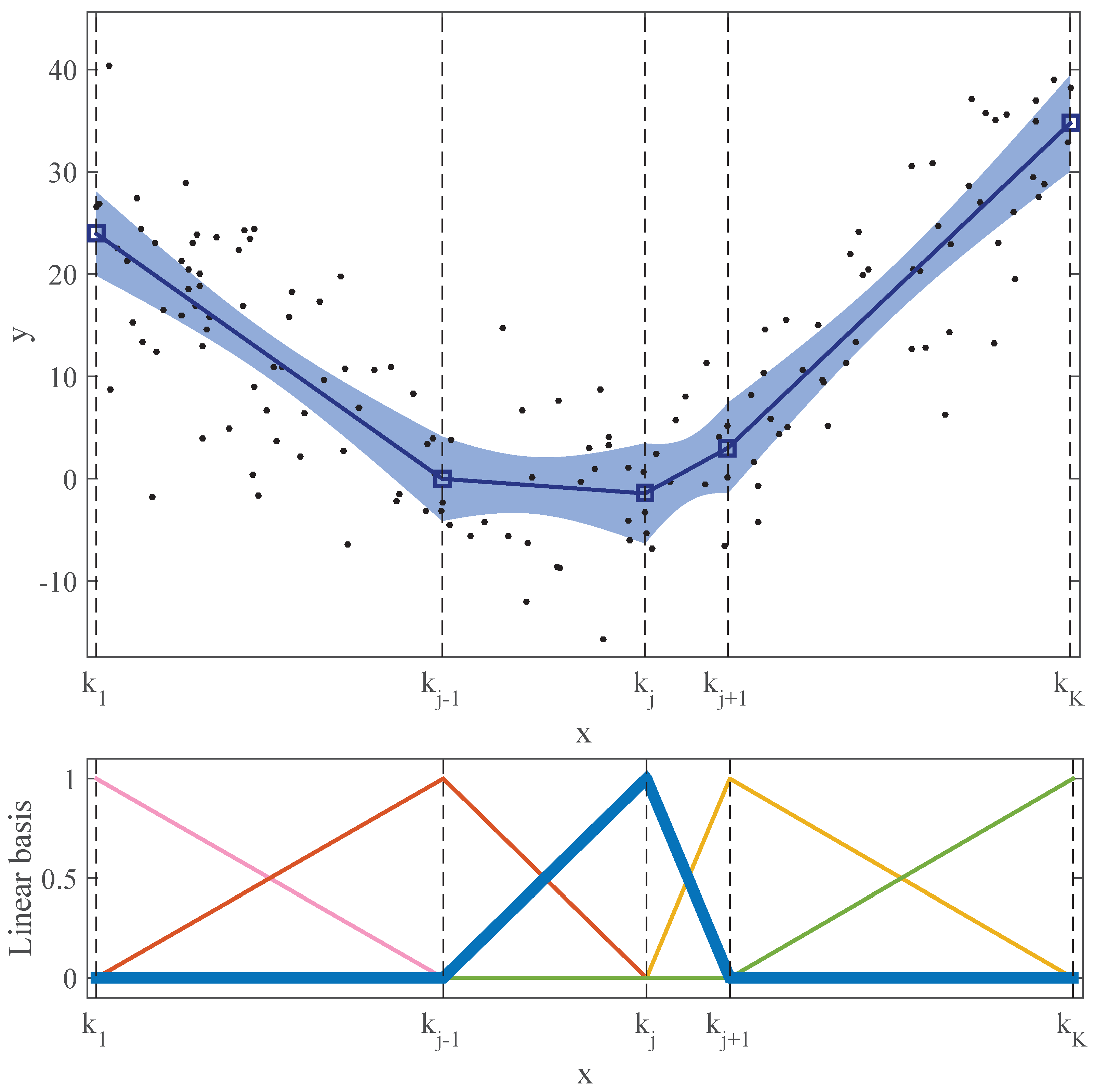
2. Continuous Piecewise Linear Regression

Continuous piecewise linear regression has been found to be helpful since it is a powerful and flexible modelling technique that allows for obtaining different functional forms. Its simplicity, together with its adaptability to any problem, have made it a very popular tool.
One-dimensional regression can be easily understood thinking about curve fitting from scatter plot data (e.g., see Figure 1, top). Consider a dataset of N points ( i = 1 , 2 , , N ) made by a one-dimensional input x and an output variable y. In addition, we will consider that each data point can have a weight w i , that is one in the standard case. The output variable is generated through the relationship (see, e.g., chapter 2 of [4])
y i = f ( x i ) + ϵ i ,
where f ( x ) is the true underlying function and ϵ i is normally distributed random noise with zero mean and constant variance σ 2 . The objective is to find a simple enough model f ^ ( x ) of the true function of Equation (1) by minimising the error, measured by the overall (weighted) mean squared error (MSE).
MSE = 1 i = 1 N w i i = 1 N w i [ y i f ^ ( x i ) ] 2 .

Model Definition

As shown at the top of Figure 1, this model can be defined as a continuous set of straight lines, linked in the knots. A model with K knots, will be made up of K 1 straight lines, with the knots being placed in the coordinates ( k j , h j ) .
These linear piecewise models can also be understood as linear B-splines and, therefore, expressed as a linear combination of triangular-shaped basis functions (see chapter 2 of [4]):
f ^ ( x i ) = j = 1 K h j B j ( x i ) ,
where each B j is a triangular basis function, possibly non-symmetric and non-zero, in the interval ( k j 1 , k j + 1 ). Therefore, the output is obtained by scaling these bases by different amounts h j , and adding them all up. Figure 1 shows a complete example of this. The continuous piecewise linear model at the top is completely defined by the combination of the set of basis functions shown at the bottom and the h j of each knot. Therefore, the model can be expressed as a set of 2 K parameters, the coordinates ( k j , h j ) of all the knots. Changing these 2 K parameters, many different shapes can be generated, with more or less flexibility depending on the value of K.

3. Parameter Estimation from Small Datasets

As already mentioned, the previous model is completely defined by the pairs of coordinates ( k j , h j ) of the knots. Hence, there are three main groups of parameters to fix: the number of knots (K), that will determine the complexity of the resulting model; their x-coordinates ( k j ), that will set the basis functions B j ; and their y-coordinates ( h j ).
In the simplest case, let us assume that the number and the x-positions of the knots are fixed, and the only parameters that must be estimated are the h j . Given the scattered data, this problem can be directly solved by using OLS, or in the more general case, when dealing with weighted input data, by applying weighted least squares (WLS). In matrix terms,
h = A 1 B T W y = ( B T W B ) 1 B T W y ,
where h = ( h 1 , h 2 , , h K ) T , B is an N × K matrix containing all the basis functions evaluated in every x-coordinate of the dataset, y = ( y 1 , y 2 , , y N ) T , and W is an N × N diagonal matrix with the weights of all the points.
Having estimated the parameters h by using Equation (4), their standard error can be also estimated as
se ( h ) = A 1 B T W σ y 2 W T B A 1 y ,
where σ y 2 is the variance of the output variable y.
In Figure 1, the confidence band around the piecewise linear model represents an estimated 99% pointwise standard error band, calculated in this way by applying Equation (5).
In the second case, when the number of knots (K) is given but their x-positions are unknown, there is no straightforward technique to fix them optimally. However, there are several different approaches in the literature, from the simplest ones, such as placing them uniformly in x or in its quantiles [10], to more sophisticated methods, such as [11,12].
Finally, the most complex case is the one in which both the complexity (K) of the model and x-position of the knots ( k j ) must be estimated. According to [4], this situation changes the regression problem from a straightforward linear problem, solved by standard least squares, to a combinatorially hard non-linear problem. In order to deal with it, greedy algorithms or two-stage processes are required.
This last case is addressed in [9], where the LHM is presented. The LHM is a continuous piecewise linear model, given by Equation (3), in which all the parameters are automatically estimated by applying a stage-wise greedy approach. A new version of its learning algorithm has been developed in this paper to be used as the fundamental piece of the models shown in the following sections. This new version follows the same strategy and steps as the former one, adding some performance improvements, but the major change that has been introduced is the possibility of using weighted data. In the Appendix A, a brief summary of the LHM’s learning algorithm is included, as well as some additional references.

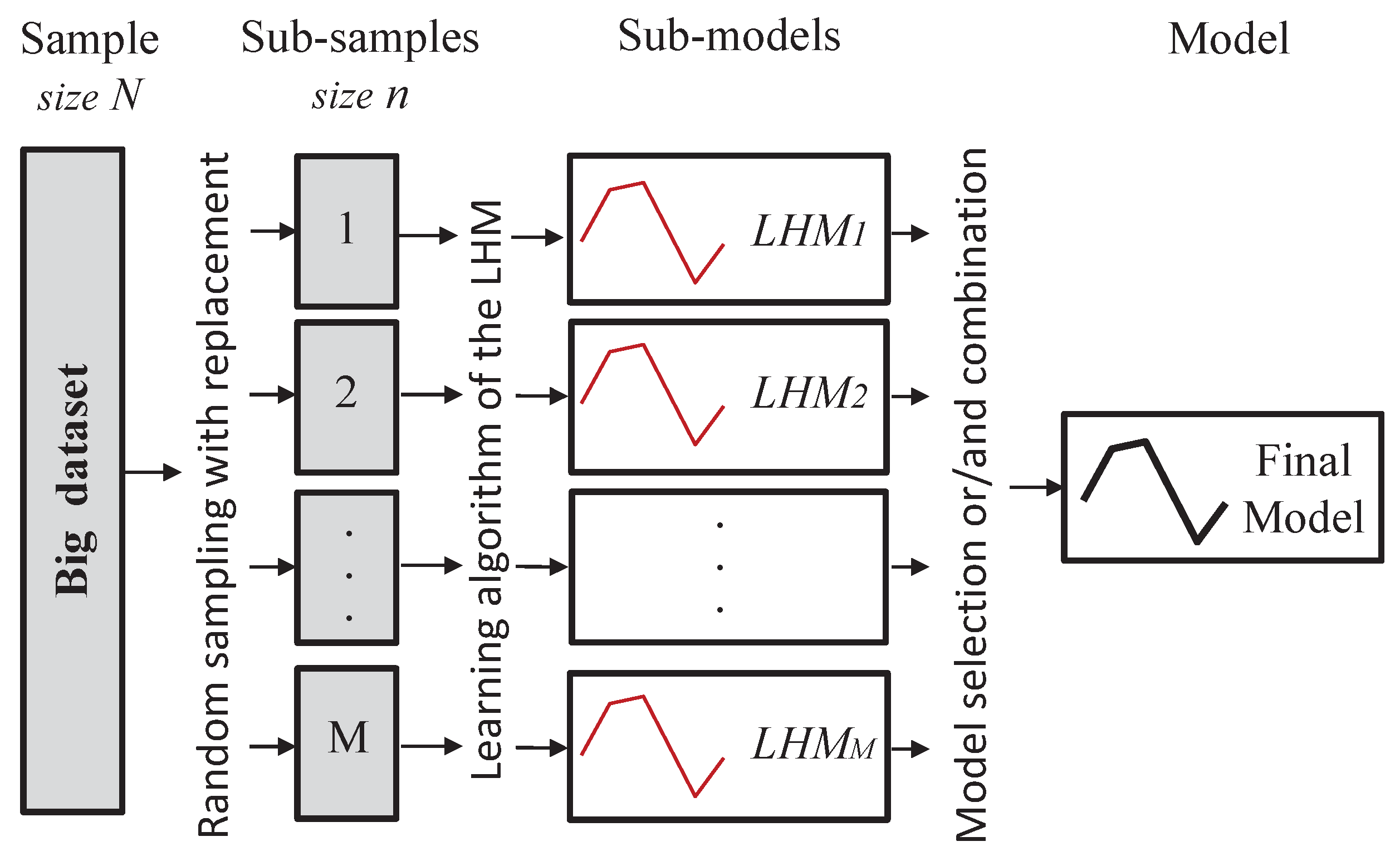
4. Parameter Estimation from Large-Scale Datasets

Previous approaches share a common practical constraint: all of them require that the entire dataset is allocated in the main memory (RAM). Thus, they are no longer valid when dealing with very large datasets. Several recent approaches can be found in the literature that adapt algorithms when data or even model parameters do not fit in the memory (see, e.g., [6,7,8]).
In the simplest case, when K and the x-position of all the knots are fixed, applying OLS or WLS would require performing operations with huge matrices. In this case, there is a large amount of straightforward solutions to scale up these matrix operations, as can be seen, for example, in [5] (chapter 5), [13,14,15,16]. Furthermore, some general-purpose mathematical programming languages and frameworks parallelise these matrix operations internally, without having to be aware of how to split them efficiently (e.g., see [17,18,19]).
However, when K and k j must also be estimated, how to scale up these methods is not so obvious. The iterative nature of the entire dataset of the algorithms that are usually applied makes them extremely difficult to parallelise and requires new approaches. For example, in [7], a new methodology for estimating a probability density function for large datasets, using adaptive partitioning and stitching is proposed. A scaling-up strategy is also required for the learning algorithm of the LHM.
There are several ways, from the most naïve to the most complex ones, to scale up the LHM learning algorithm to large-scale datasets. Among possible alternatives, in this paper, we focus on model selection and combination techniques. The first general approach would be using simple random sampling, where a (small) sample of size n < < N , constrained by the available memory, is used as input for the traditional algorithm. This solution would have the advantage of being the simplest and fastest one. However, it has an important drawback: it would not be taking advantage of the richness of the data. In the case of a problem with a very complex structure, or with a lot of noise, the sample size can be insufficient to determine K properly, and therefore, the final model can have a high generalisation error.
Model selection techniques aim at choosing a model from a set of candidates. Based on the previous approach, after taking several samples and estimating the parameters in each one, we could apply a selection technique, such as BIC [20], AIC [21], or cross-validation to decide the best model in terms of both complexity and accuracy. This option would be better than taking only one sample, but it shares with that approach the problem with complex underlying structures and noisy datasets.
Model combination consists of building a series of sub-models, each with a data partition, and finally combining them somehow. Model combination has been proven to be a good solution to deal with the uncertainty of model selection and has been demonstrated empirically to outperform it [22]. Applied to regression analysis, many combination methods, such as bagging or boosting, have been proposed. Bagging consists of combining by averaging several bootstrap samples (with replacement and of the same size as the input dataset), and its main goal is to reduce variance [23]. On the other hand, boosting [24] aims at iteratively improving a weak model to reduce bias and variance. These methods, initially designed to improve the accuracy of a model, are suitable tools when dealing with very large datasets of size N. They allow for taking advantage of the full dataset by improving the models that can be obtained from samples of size n < < N .

5. Proposed Methods

In this section, we present the proposed and tested approaches in order to obtain a piecewise linear regression model from a very large dataset using the learning algorithm of the LHM. All the implemented methods are based on the same idea (see Figure 2): take several sub-samples of the dataset, constrained by the available memory, fit an LHM to each one using the standard learning algorithm described in [9], and finally, collecting all the sub-models, build a unique model. Note that there is not a clear approach to obtain a final model from this set of sub-models. As mentioned in the previous section, we could simply choose one by applying a model selection technique or combine them in a more elaborate way. Furthermore, there are many different possibilities to combine these piecewise linear models. Figure 3 shows an illustrative example, where several sub-models have been built from sub-samples of n = 1000 data points. It can be seen that, in spite of the fact that all of them have similar shapes and are also similar to the true underlying function, there is a lot of uncertainty in the position of the knots.
Finally, a combination of these two approaches may be advantageous in some cases. For example, in [22], the authors discuss whether to use model selection or combination, and propose a combination method for linear regression models that incorporates an initial screening step to exclude very poor models from the subsequent combination.
In addition to selecting a proper way to obtain a model from these sub-models, there are two other important parameters that must be previously selected and also affect the final result. First, the sub-sample size n is decisive due to the fact that it can lead to poor sub-models when n is not large enough to be a representative sample. Second, the number of sub-samples is also relevant since increasing M will lead to more robust models.
In the following subsections, several approaches to model selection and combination are presented. Subsequently, Section 6 presents empirical results using these methods, as well as an analysis of the impact of changing M and n in the final result.

5.1. Model Selection (MS)

This approach can be considered the simplest one: the parameters of the resulting model will be fixed by the best model selected from the set of candidate sub-models, each one estimated using a different sub-sample. In order to select it, first an extra sample is reserved as test set (TS), and then, the Bayesian information criterion (BIC) [20] is used, because it provides a good compromise between error and complexity. The BIC is a statistical measure used for model selection that balances goodness of fit with model complexity, penalising overly complex models to prevent over-fitting. For each sub-model, it is defined as
BIC ( LHM s , TS ) = log ( MSE ( LHM s , TS ) ) + K s n log ( n ) ,
where MSE(LHMs,TS) is the MSE of sub-model s calculated by applying Equation (2) over the TS, and K s its complexity (number of knots). Applying this method, the BIC of each sub-model is calculated, and the one that presents the lowest value is finally selected.

5.2. Model Combination (MC)

In this subsection, the proposed combination methods are presented. In all of them, the sub-models have been considered equally relevant. According to Figure 2, once calculated, the M sub-models LHM1, LHM2, …, LHMM build a unique piecewise linear regression model by combining them somehow. Let us denote K s the complexity of the sub-model s, and let k s = ( k 1 s , k 2 s , , k K s s ) T and h s = ( h 1 s , h 2 s , , h K s s ) T be the x- and y-coordinates of its knots, respectively. The final model (LHM) will be defined by the sets of coordinates ( k , h ), having K knots.

5.2.1. Output Averaging (MC1)

This combination approach can be considered the naïve one since it consists of simply averaging all the set of sub-models in several points. As shown in Figure 3, once the M sub-models have been obtained there is a lot of uncertainty about the number and position of the knots. In this method, the knots are fixed to a predefined number of equally spaced points. In our simulations, a grid of 10,000 points has been used. Therefore, fixing the number (K) and x-positions ( k j ) of the knots of the final model, their y-positions can be calculated as
h j = 1 M s = 1 M LHM s ( k j ) ,
where LHM s ( k j ) is the output of sub-model s evaluated in the x-coordinate k j . Note that since the data noise has been previously filtered by applying the LHM to each sub-sample, this model will not have over-fitting, even when it is over-parameterised. It is also worth mentioning that this combination method produces non-structured models. Instead, a look-up table with the expected output at several values of x is given. Due to the high value of K, little effort has been made to remove useless knots. In fact, pruning them in a traditional greedy way would be computationally expensive.

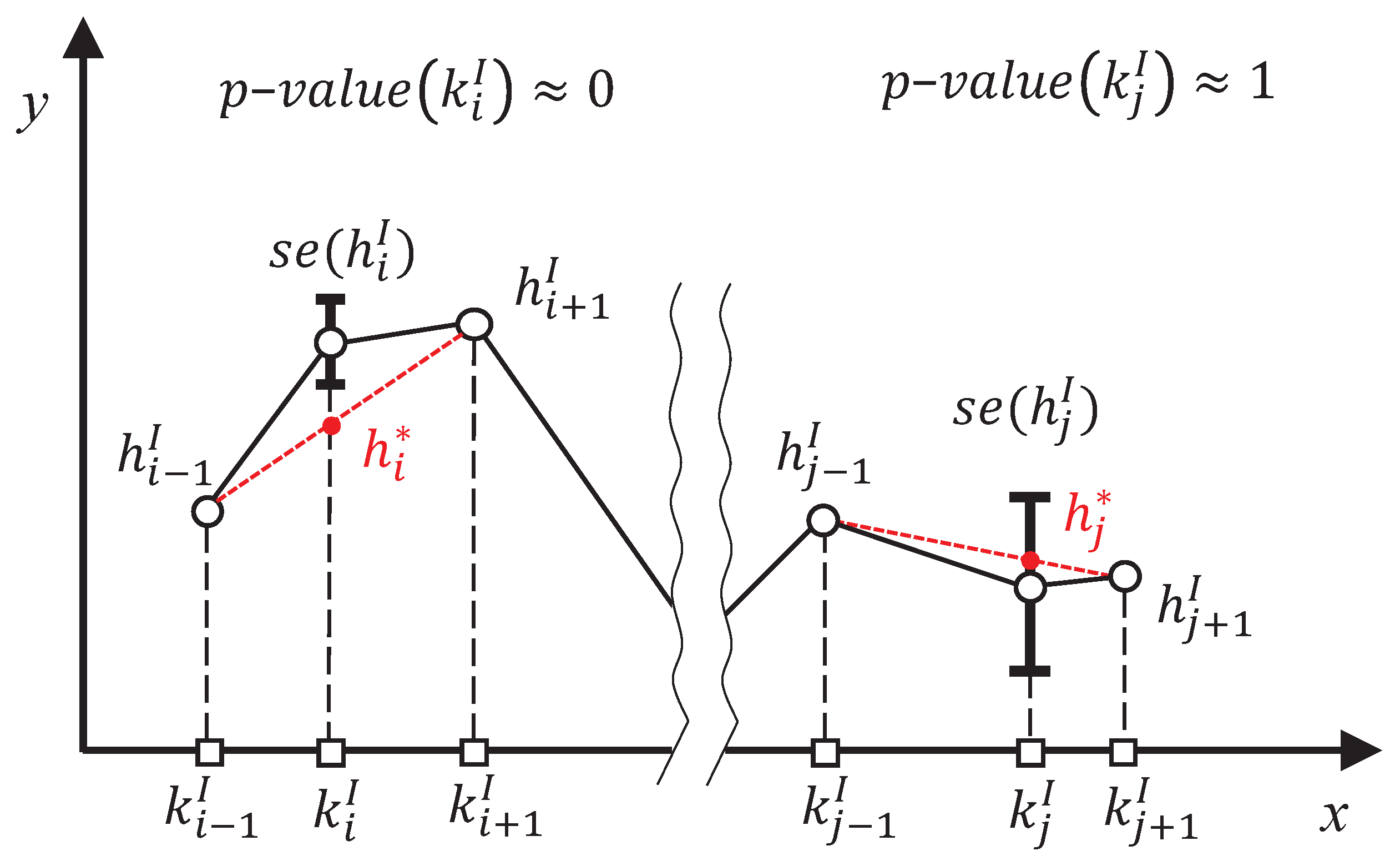
5.2.2. Model Averaging with Complexity Reduction and Refitting (MC2)

This approach, unlike the previous one, selects the number and position of the knots in a more clever way by taking into account the location of the knots of the M sub-models. In this way, the zones where f ( x ) changes more rapidly or has greater curvature will present a higher number of knots than those that can be easily represented by a reduced number of straight lines. The overall strategy resembles the original learning algorithm of the LHM, consisting of three consecutive stages. First, an initial model is built from the sub-models using a straightforward growing approach (based on model averaging). Then, the irrelevant knots are iteratively pruned, and at the end, the pruned model is refitted to obtain the final one.
In order to build the initial average model, an initial set of knots is fixed as
k I = ( k 1 k 2 k M ) = ( k 1 I , k 2 I , , k K I I ) T ,
where K I is the complexity of this initial model. Once the number of knots and their x-positions are fixed, their h j I are calculated by applying Equation (7) to each x-coordinate of k I . This model is usually over-parameterised and requires a pruning step. A new pruning algorithm has been developed in order to address this problem. The main idea of this approach is to reduce iteratively the complexity of the average model, taking into account the dispersion of the set of sub-models in each knot, estimated as
s e ( h j I ) = 1 M · ( M 1 ) s = 1 M ( h j I L H M s ( k j I ) ) 2 .
This pruning step aims at selecting a subset of the initial knots ( k I , h I ), taking into account the dispersion of the set of sub-models at each one. Thus, a pruning sequence of models of decreasing K is iteratively built, removing the less relevant knots one by one, and then, the best model of the sequence is selected according to the p-values of their knots. The general procedure of the pruning algorithm is described in Algorithm 1. Let us denote as h j * the y-coordinate obtained from evaluating the line that connects the points h j 1 I and h j + 1 I in k j I (see Figure 4). Assuming that the y-coordinate of each knot of the initial model follows a normal distribution of mean h j I and standard deviation s e ( h j I ) , the relevance of each knot is determined by the p-value of the point h j * given the previous normal distribution. In each iteration, the knot with the highest p-value calculated in that way is pruned. An example of one iteration of this method can be seen in Figure 4, where the knot ( k j I , h j I ) would be pruned due to the fact that the value of h j * is very close to h j I .
Algorithm 1 Pruning algorithm of MC2.
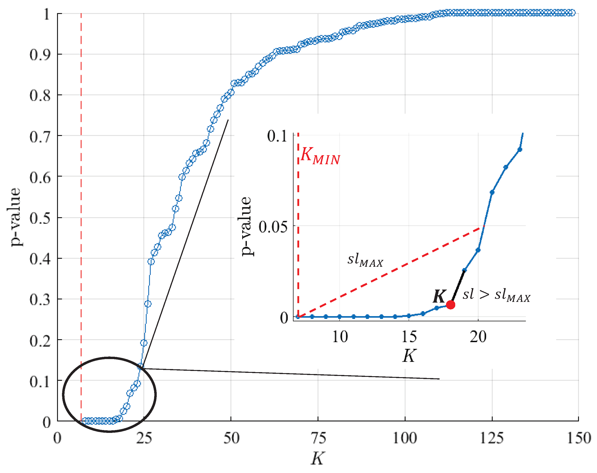
PART I: Generate the pruning sequence
(a) initialisation
k = k I , h = h I
P M m = K I = k , h , K m = K I = K I
for  m = ( K I 1 ) down to K m i n  do
    (b) calculate the p-value of each knot
    for  j = 2 to ( K m 1 ) do                  ▹ for all the internal knots
         h j * = k j k j 1 k j + 1 k j 1 · ( h j + 1 h j 1 ) + h j 1
         p j = p -value ( h j * ) with N ( h j , s e ( h j ) )
    end for
    (c) prune the knot with the highest p-value
     k = k k d , h = h h d where d = arg max j p j
     P M m = k , h
    (d) save the p-value of the pruned knot ( p m ) and K m
     K m = K m + 1 1 , p m = p d
    (e) calculate the slope of the p-value curve in m
     s l m = p m + 1 p m K m + 1 K m
end for
PART II: Select the final PM and K
(a) calculate the maximum slope that is allowed
s l m a x = 0.05 p K m i n K 0.05 K m i n
(b) find the elbow of the p-value curve
f = s l > s l m a x
(c) select the final K and P M
K = K f ( 1 ) , P M = P M f ( 1 )
Given the maximum complexity ( K I ) and fixing the minimum one to the lowest K s of the sub-models ( K m i n = m i n ( K 1 , K 2 , , K M ) ), the pruning sequence of the models is built by pruning the knots one by one in that way. In each iteration m, the pruned model ( PM m ) is saved, as well as its complexity K m , and the p-value of the last knot that has been pruned ( p m ). Therefore, once the pruning procedure has finished, a set of K I K m i n models is obtained, each one associated with the p-value of the knot that has been pruned in its iteration. Figure 5 shows the p-value sequence for each PM after the whole pruning process. It can be observed that, as expected, the p-value of the knots decreases during the process, pruning from the most irrelevant knots with p-values near 1 to some of them with p-values very close to 0.
Once the pruning sequence has been built, the final complexity K is selected by looking for the elbow of the p-value curve (see Figure 5). Specifically, the last point of the curve with a lower slope than the one given by the line that connects the end point of the pruning sequence and the point of p-value = 0.05 is chosen. The selected model after the pruning step is the PM of the sequence with that value of K.
Finally, a refitting step is carried out to improve the knots’ positions. For this, a new cloud of points is created, evaluating the sub-models in several x-coordinates. Constrained by the available memory, the number of points for this final step (Q) is fixed. In this paper, Q is fixed to 500 k. Then, each sub-model is evaluated in a random set of x-coordinates of size Q/M. These points are uniformly generated over the x-range to avoid repetition in different x-coordinates as much as possible. Once this new dataset is generated, the refitting step of the original LHM algorithm is executed (its details can be seen in [9]), fixing the final position of the knots of the model.

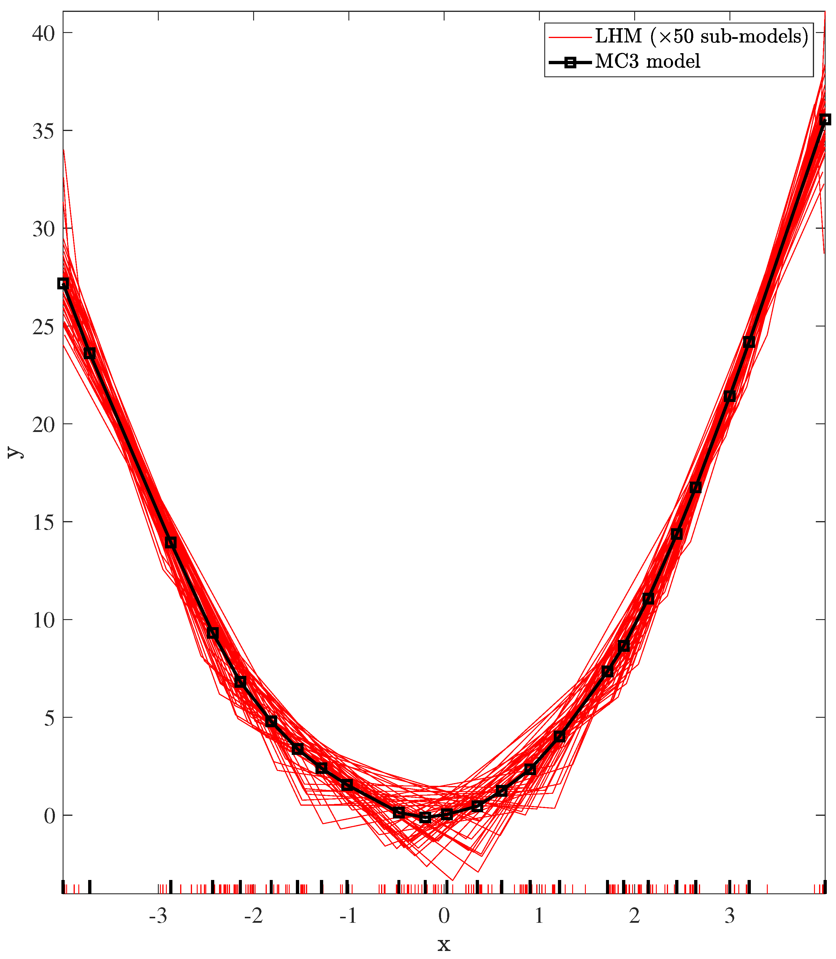
5.2.3. Applying the Learning Algorithm of the LHM to the Set of Sub-Models (MC3)

This combination approach is based on the reference algorithm and treats the sub-models as a new learning set. Using the new dataset of size Q described in the previous method, made by evaluating the M sub-models in random sets of x-coordinates of size Q/M, the reference algorithm is fitted to these data. Figure 6 shows an example of this: the 50 sub-models fitted with n = 1000, and shown in Figure 3, are used to build the new input dataset, and after applying the reference algorithm, the plotted piecewise linear model is obtained.

5.3. Improving MC by Means of OLS

In spite of the fact that all the proposed methods provide a continuous piecewise linear regression model that could be considered the final one, the position of their knots can be improved, due to the fact that a final OLS can be carried out. Note that this approach can produce better models only if the model is not over-parameterised, i.e., when the model’s flexibility has been explicitly limited by selecting the lowest complexity, providing an acceptable generalisation capability. Clearly, this is not the case of the output averaging method (MC1). Thus, the proposed MS, MC2, and MC3 can take advantage of this final optimisation. Once the basis functions B j have been fixed, using a model selection or combination method, their final h j can be estimated by using OLS (Equation (4)) with the full dataset, by applying efficient matrix decompositions. The next section presents a comparative analysis of all the proposed methods, where the effect of performing this final optimisation step is also tested.

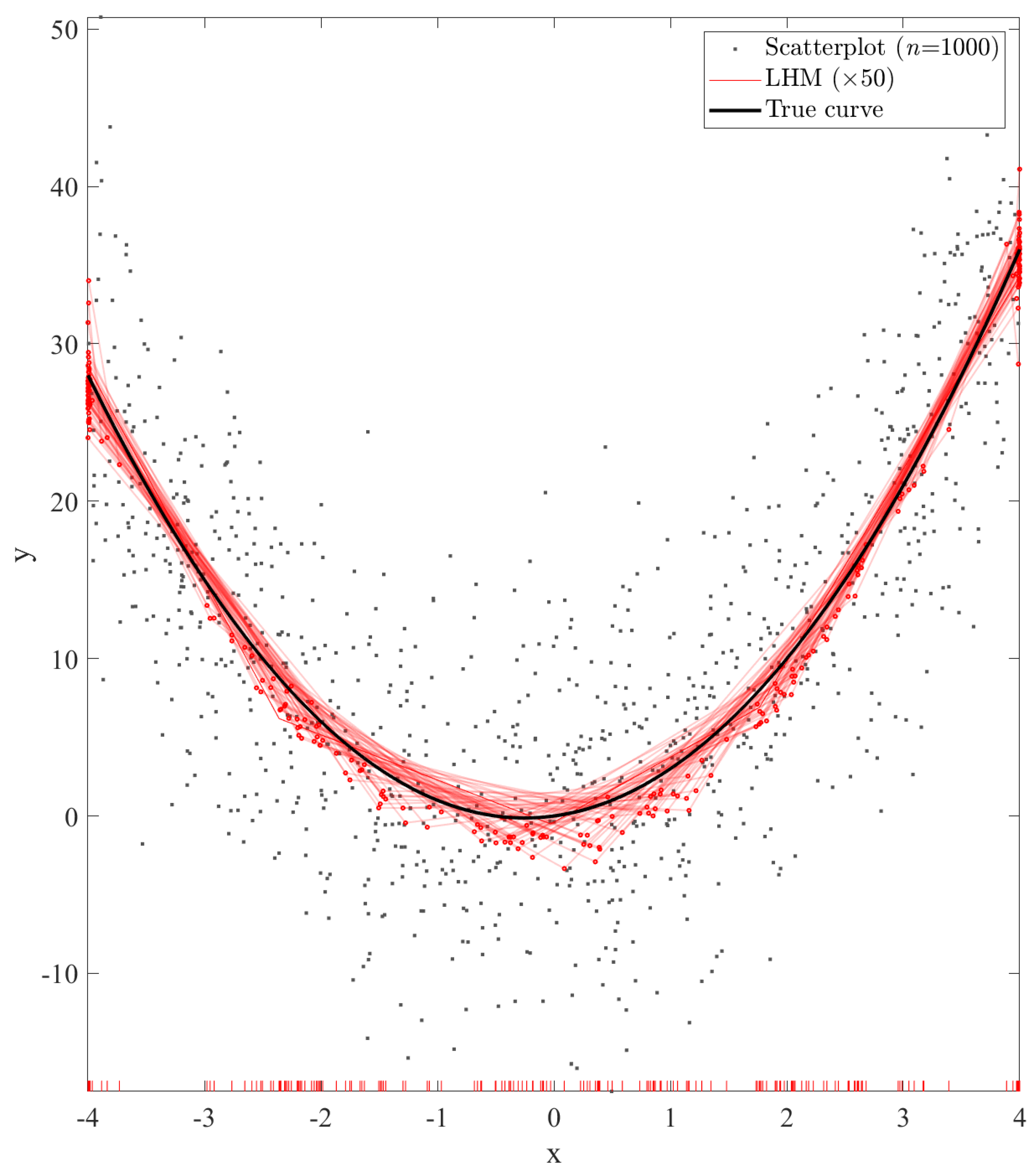
6. Empirical Results

In order to test all these different approaches, a Windows server with an Intel Xeon E5-2660 (2.6 GHz) processor (10 cores), 144 GB of RAM, and an SSD of 500 GB was used. All the implementation was carried out in Matlab R2022b, using the Parallel Computing Toolbox.
As shown in Table 1, four different problems with different sizes and complexities were used for testing. Following Equation (1), additive random error ( ϵ ) was generated according to a normal distribution of zero mean and standard deviation σ = 0.2 · range ( f ( x ) ) . Figure 7 shows an example of each problem. The empirical results of the proposed methods in all these problems are shown at the end of this section (see Section 6.5), but for simplicity, and in order to illustrate their behaviour, only the simplest (PR1) and the most complex one (PR4) are used in the other subsections.
For each problem, 30 independent datasets with 10 million instances were generated as scattered learning sets (SLSs), as well as an independent one of 500 k points for the scattered test set (STS). In addition, to measure the error with the true underlying function, a set of 50 k data without noise was used as the true test set (TTS). All this section’s quantitative results and graphs are calculated from these 30 replications.
In order to test the performance of all the proposed methods, their results are compared with the ones obtained with the reference algorithm (LHM) executed over the full datasets of 10 million data. The combination and selection methods are based on sub-samples of sizes (n) between 1 k and 1 M data, and different values of M.

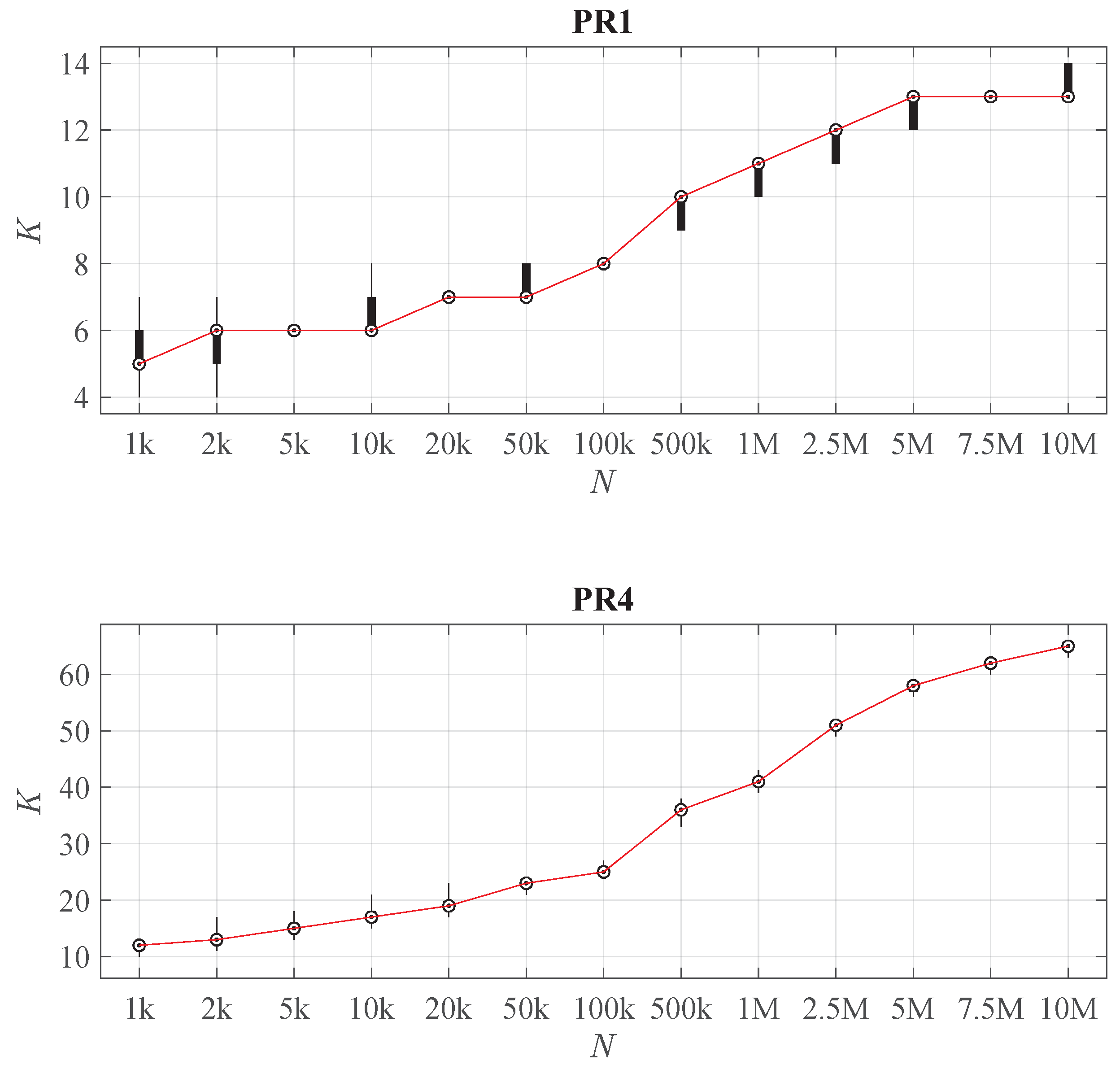
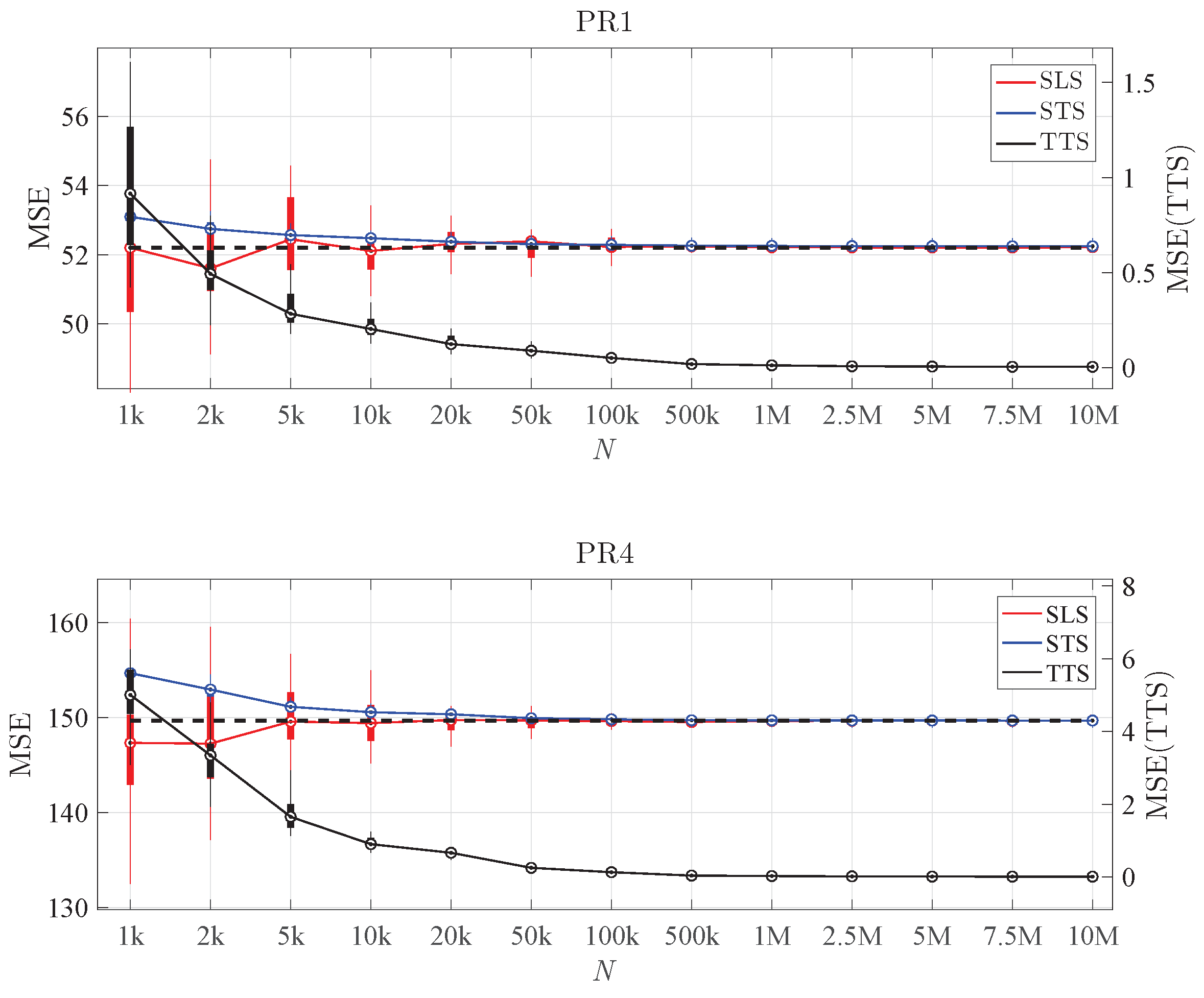
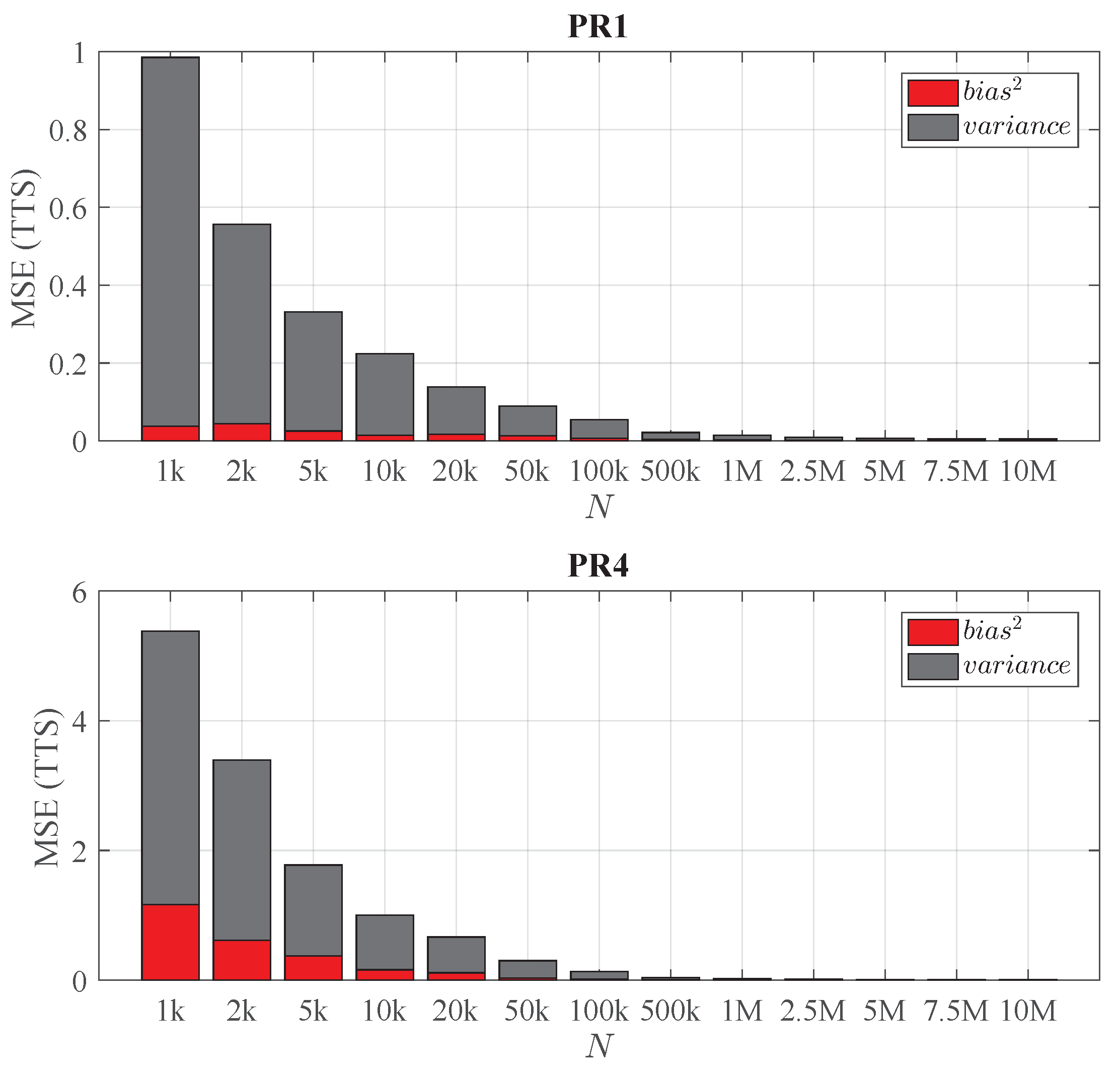
6.1. Performance of the Reference Algorithm

Since the selection of the size of each sub-sample is determinant in the final result, an initial analysis of the performance of the standard LHM learning algorithm when varying the number of points was carried out. It is clear that for the same noise level, the more input data we use as the training set, the lower error we achieve.
First, in order to illustrate the differences between the models obtained from different values of N, Figure 8 shows LHMs obtained from a small and a big sample size. It can be seen that by increasing N from 1 k to 100 k, we can reach a great improvement in the accuracy of the model. Using a small SLS, we obtain a ’weak’ model, whereas with N = 100 k both the accuracy and complexity (K) of the model increase.
This increasing complexity of the LHM with N is systematic in those problems. According to Figure 9, K continuously grows with N. Note that its growth ratio decreases with N, i.e., larger increments in N are required to produce an effective increase in K. Furthermore, for a given sample size, there is a small dispersion around the median value of K, so it can be concluded that the learning algorithm of the LHM estimates the complexity in a robust way.
Regarding the error of these models, Figure 10 shows their MSE over the different datasets. It can be seen that, as expected, the MSE(TTS) decreases with increasing N, and both MSE(SLS) and MSE(STS) stabilise around the variance of the noise. Despite having more and more knots when N increases, these models are not over-fitted, being more and more accurate. Therefore, we can conclude that the reference algorithm does a reasonable job by adapting the estimated model’s complexity to the underlying structure’s complexity and the amount of available data.
Finally, in order to achieve a deeper knowledge of the performance of the reference algorithm, the MSE can be broken down more finely. It is well known that the MSE over the TTS can be decomposed in two terms (see, e.g., [4]):
MSE ( TTS ) = b i a s 2 + v a r i a n c e .
The first term is the b i a s 2 , and it measures how closely the average model (given the set of models estimated from different samples of the same size) matches the true function. The second term represents the variance of those models from the average one, and it measures the certainty of the estimated models for a given sample size.
Figure 11 shows this decomposition of the MSE(TTS) of the LHMs when varying N. It can be seen that in both problems, most of the error is due to the variance, especially when the SLS is small. Furthermore, the bias and variance decrease rapidly when N increases. Comparing the results obtained from the different problems, it can be observed that the simplicity of PR1 results in a much lower error than the one obtained in PR4. In PR4, for very small sample sizes, a high bias is obtained due to the fact that the algorithm is not able to recover the most complex part of the underlying structure. However, in PR1 the bias obtained even with small values of n is quite small compared with the total error. This empirical evidence shows that, in terms of accuracy, there is room for improvement, especially by means of reducing the LHM variance. The proposed combination methods take advantage of this fact.

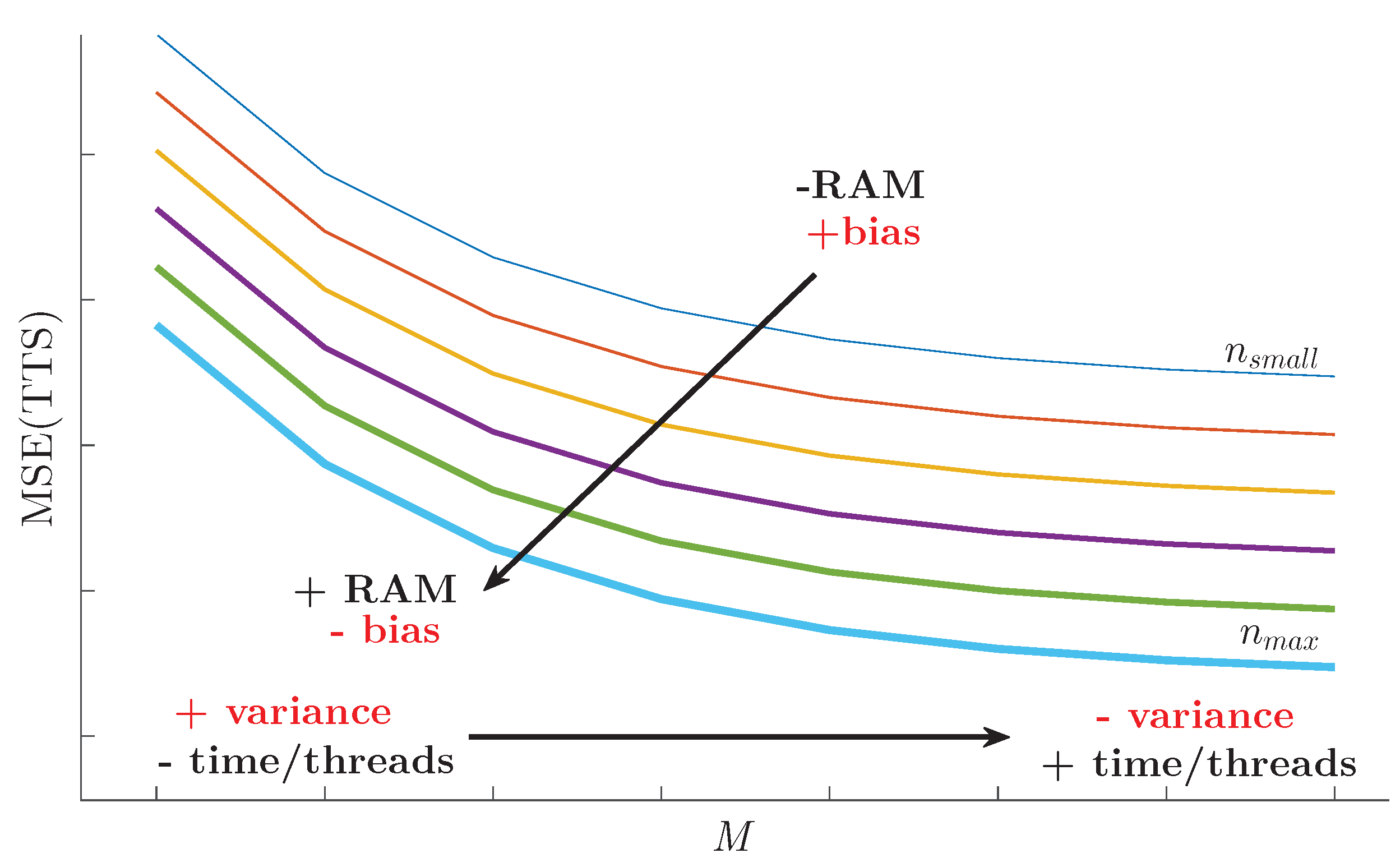
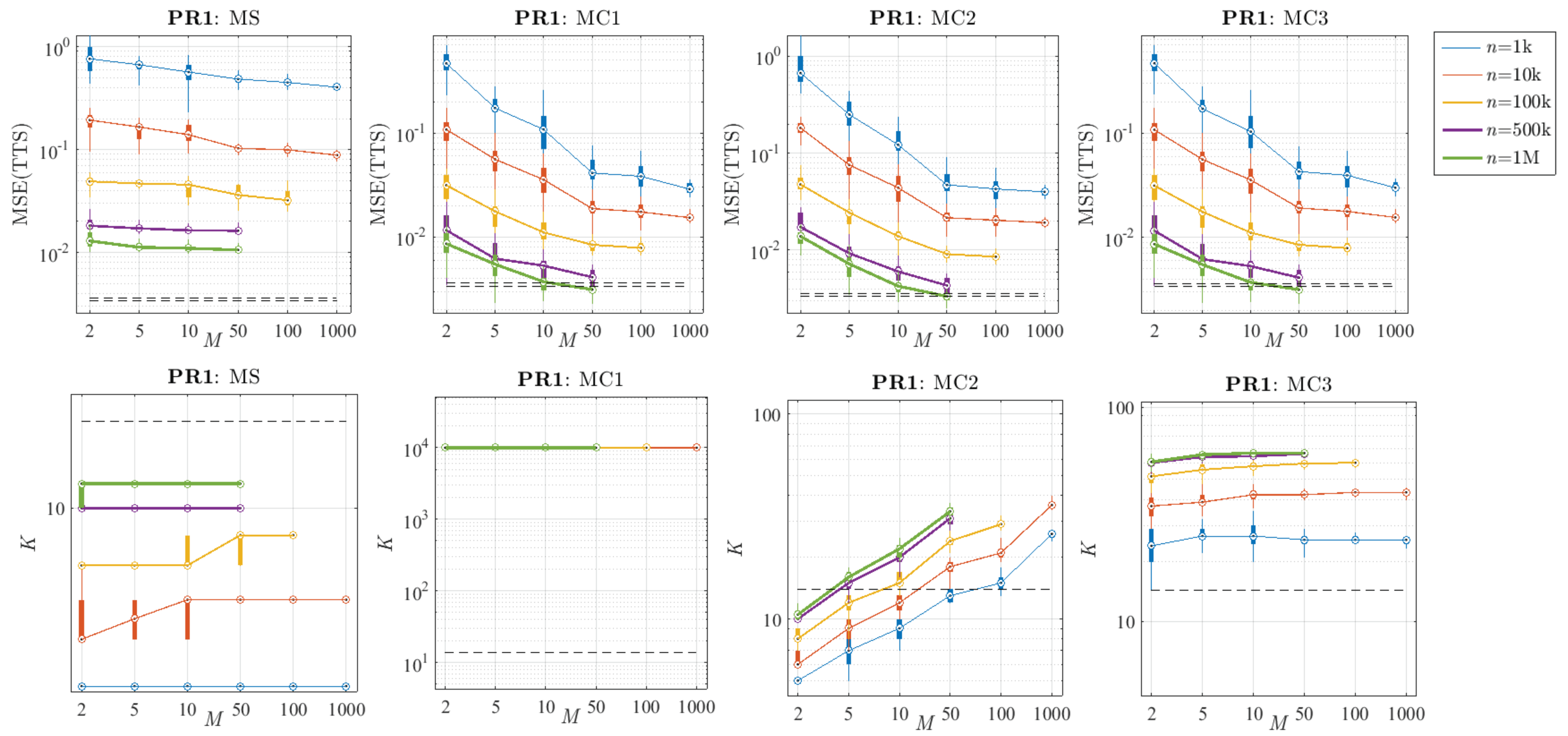
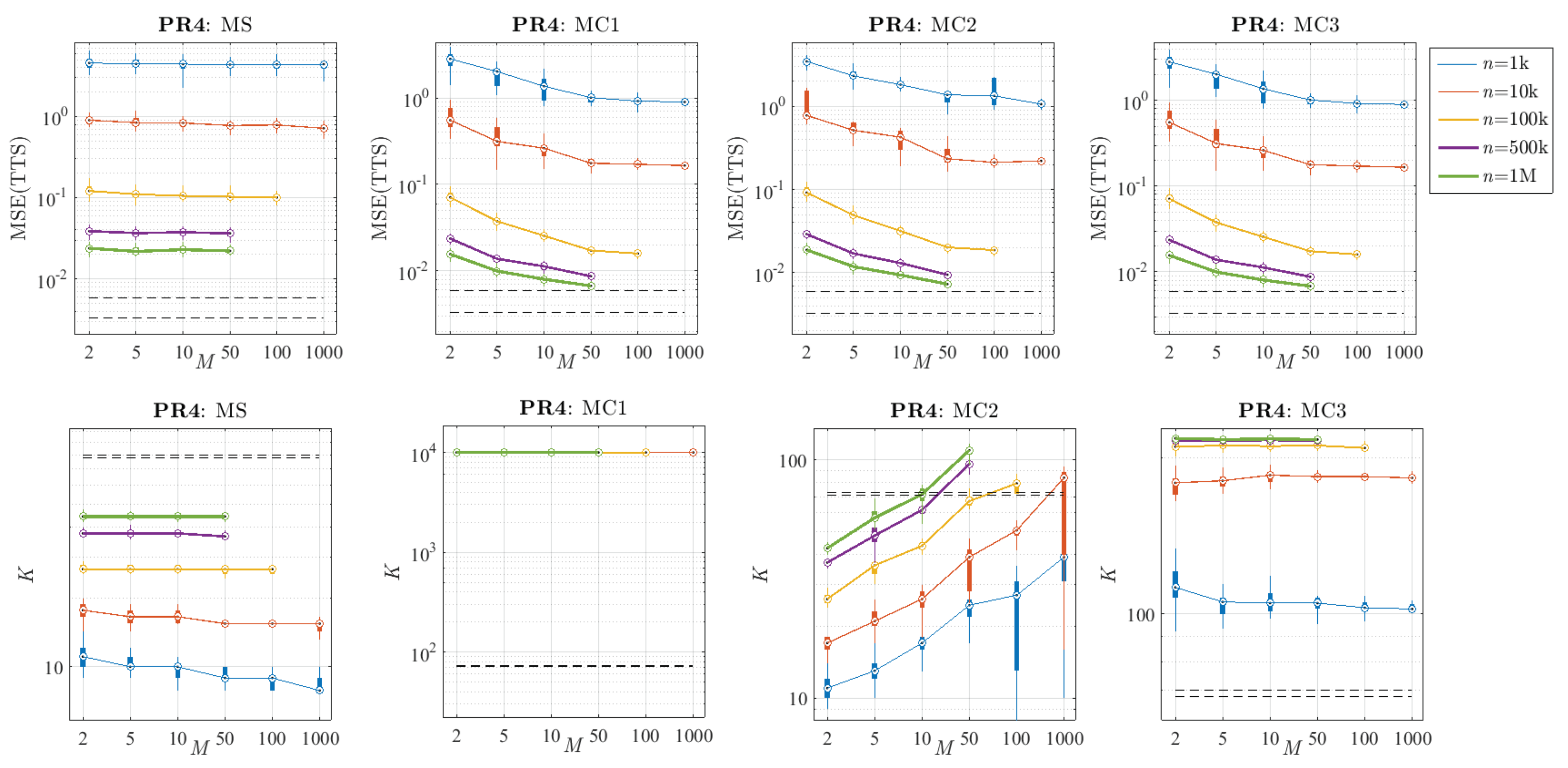
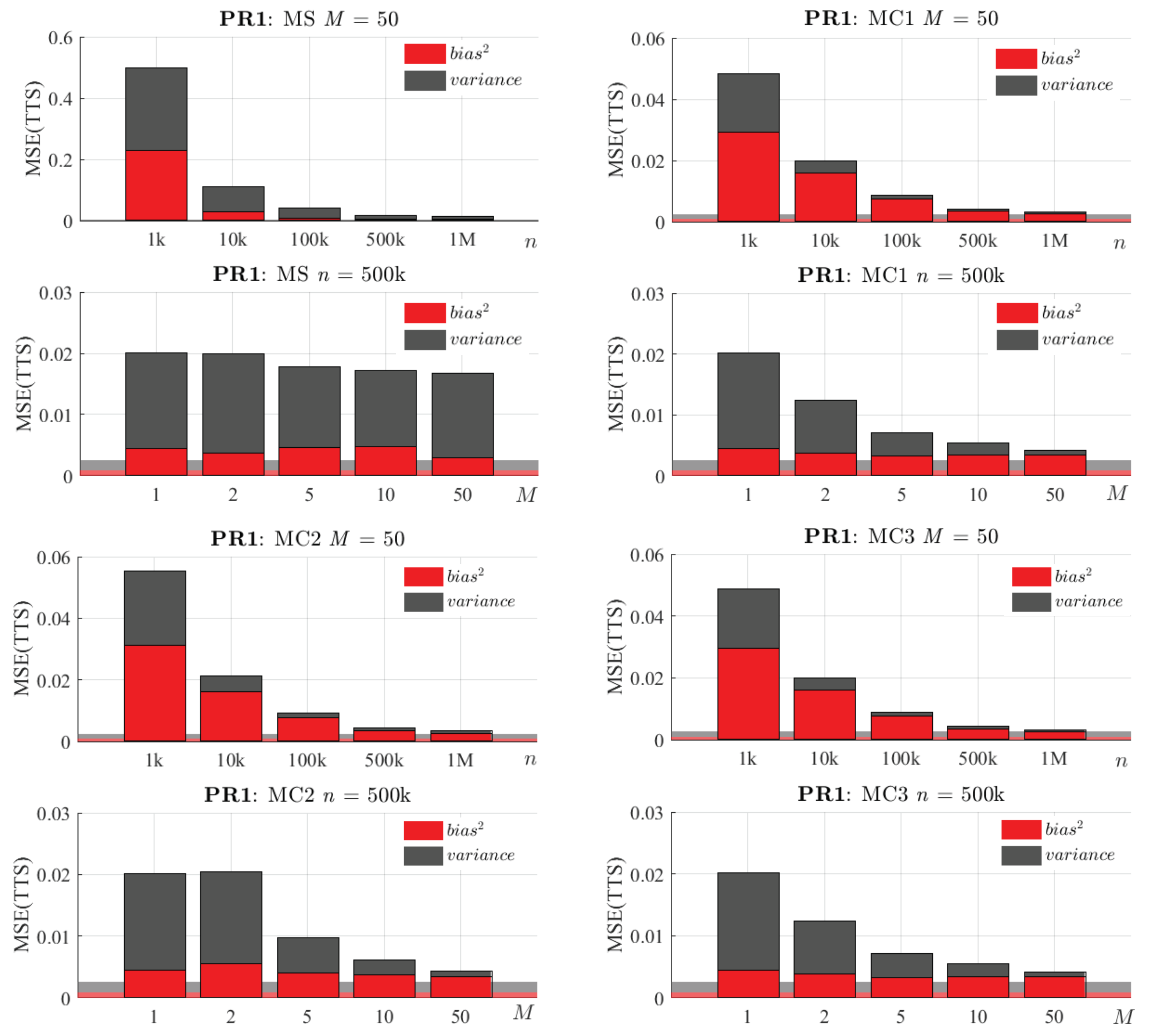
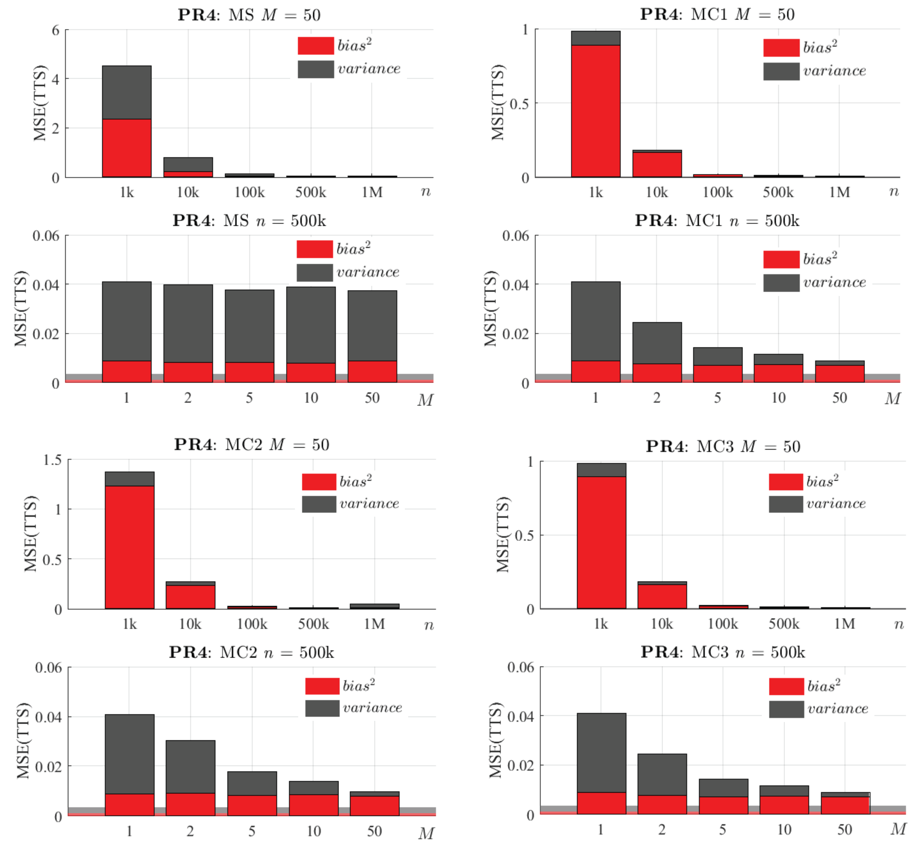
6.2. Selection of n and M

This section will focus on the behaviour of the different selection and combination methods varying n and M. As shown in the previous section, it is clear that the sample size is determinant in the accuracy and complexity of the LHM. Furthermore, different levels of noise and problem complexities will require different sample sizes in order to obtain models of the same quality. Since the LHM always improves its accuracy with increasing N, the sample size should be large enough to allow the learning algorithm to separate the noise from the underlying structure of the problem. On the other hand, for a fixed n, an increase in the number of sub-samples (M) also produces more and more accurate models.
Figure 12 summarises the performance of all the combination methods when changing the sub-sample size as well as the number of sub-samples. It can be seen that in order to reduce the bias an increase in n is required, always constrained by the available RAM. In addition, we can achieve a variance reduction by increasing the number of sub-samples. This would result in an increase in CPU-time or, since they are independent processes, the number of threads if concurrent execution is available.
In order to assess empirically the impact of these two parameters in the final model, the performance of all the methods was compared, varying n and M in each problem. For example, Figure 13 and Figure 14 show their systematic behaviour when changing these parameters. As expected, according to the results of the reference algorithm, higher values of n also bring better results in terms of accuracy when combining several LHMs. Furthermore, the method based on model selection (MS) always has flatter error curves than the ones based on combination. In spite of the fact that the bias is reduced by increasing n (in the same way as for the reference algorithm in Figure 10), the MS method does not reduce the variance in the reference algorithm since it is calculated in the same way. Regarding the combination methods, it can be observed that the shapes of their error curves are quite similar in every case.
Further insight about the origin of these reductions in the MSE can be found in its bias–variance decomposition. Following Equation (10), the MSE(TTS) was decomposed in these terms. Figure 15 and Figure 16 show that, as expected, an increase in n causes a decrease in both bias and variance. In addition, increasing M significantly reduces the variance, whereas the bias remains approximately constant.
Regarding the impact of n and M in the complexity of the final models, the bottom of Figure 13 and Figure 14 show the K curves when varying those parameters. As shown in Figure 9, the reference algorithm fixes higher and higher complexities when increasing the sample size. Therefore, a similar behaviour is expected from the methods MS, MC2, and MC3 (the number of knots of MC1 is always fixed). However, the effect of changing the number of samples is not so obvious a priori, with the exception of the method based on model selection: since the reference algorithm is robust in fixing K given n, having more candidate sub-models will not change the final K too much.
Comparing methods MC2 and MC3, it can be seen that they have a very different behaviour with n and M when deciding the number of knots. Method MC2 provides larger and larger values of K when increasing M, whereas MC3 has flatter complexity curves, being more stable in fixing the number of knots. Furthermore, note that MC2 requires a larger number of sub-samples to reach the complexity fixed by the reference algorithm and presents higher dispersion in its complexity curves (see Figure 14, bottom), so that it seems to be less robust when fixing K. On the other hand, MC3 systematically overcomes the complexity of the reference algorithm, even for small values of M. Due to the fact that, as is shown in Figure 2, these methods are not over-fitted even with higher complexities than the reference algorithm, obtaining larger values of K usually provides more accurate models. This confirms that we can obtain models with higher complexities than the reference algorithm, with even less generalisation error.

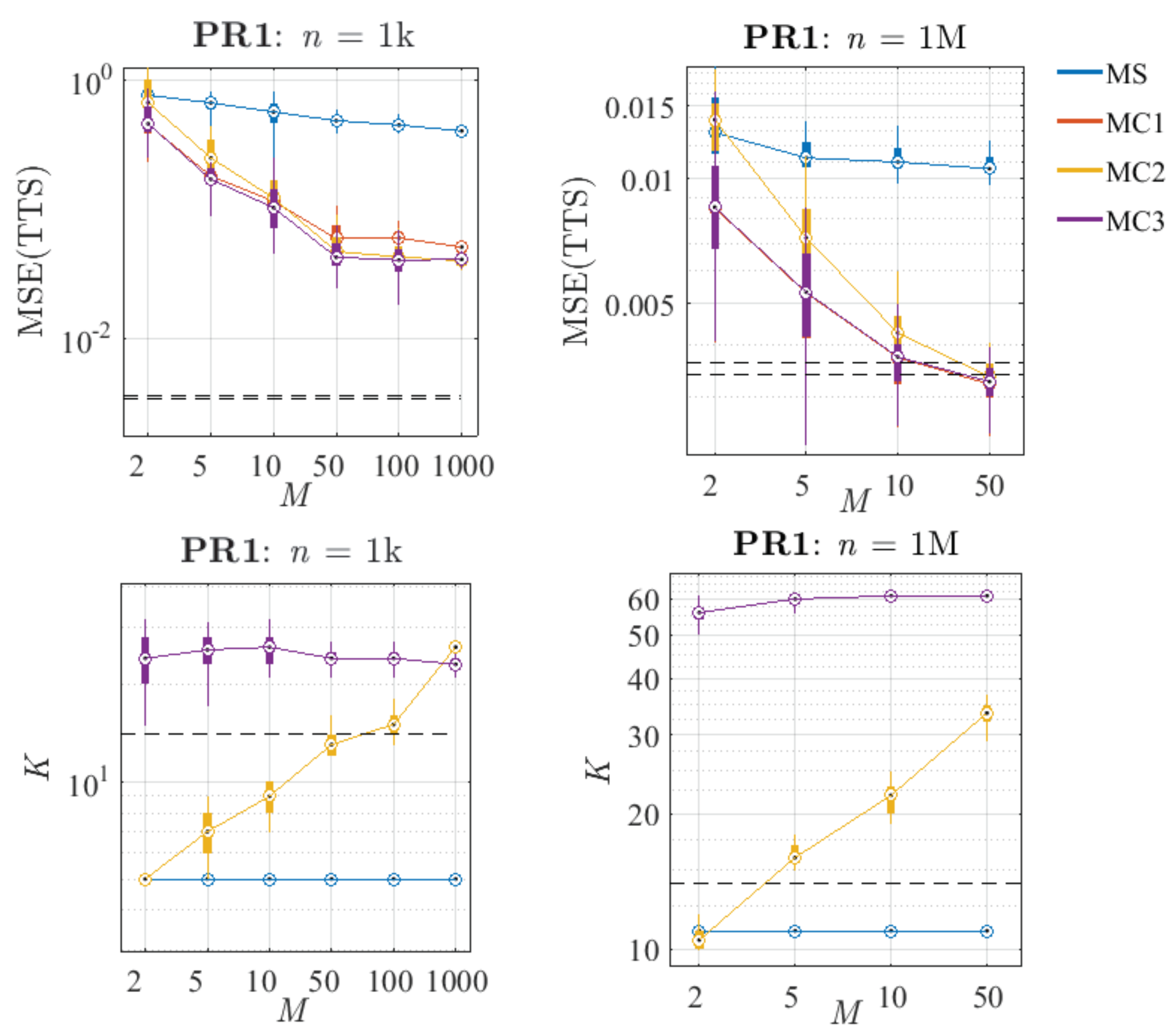
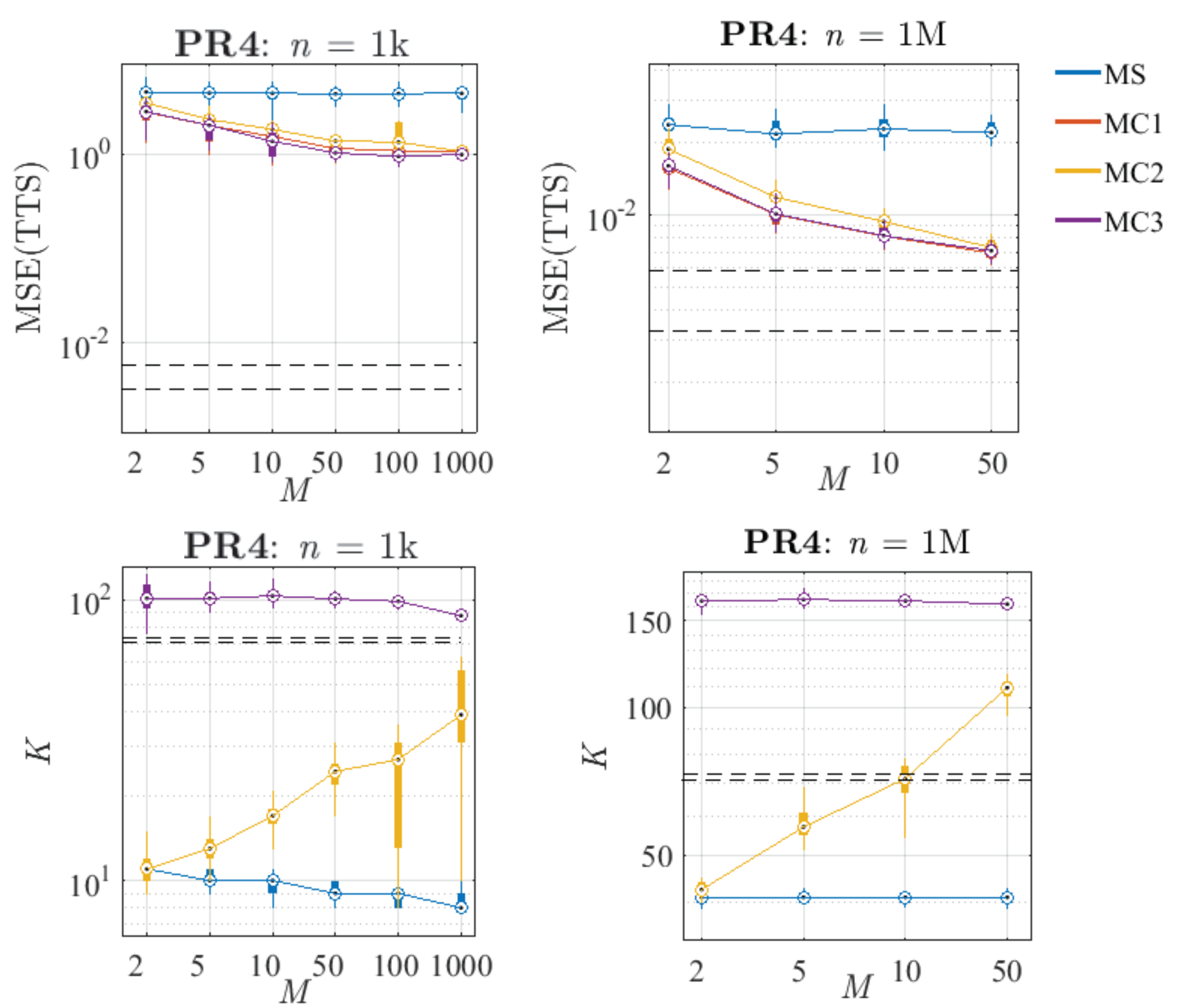
6.3. Comparative Analysis of the Proposed Methods

As summarised in Figure 12, all the tested combination approaches behave in the same way when increasing n and M: they improve in terms of bias and variance. The model selection, as expected, does not take advantage of increasing values of M to reduce variance, and it only improves with increasing n in the same way that the reference algorithm did.
This section aims at comparing the performance of the proposed methods. In particular, Figure 17 and Figure 18 present the error and complexity curves of the methods for a small and a large sub-sample size. Both figures clearly show that MS is always the worst option because it produces models with the highest generalisation error. Note that the complexity of these models is always lower than the K chosen by the reference algorithm because of the fact that BIC selects one model among under-parameterised LHMs.
Regarding the combination methods, it can be seen that when a small value of n is chosen, the MSE(TTS) stabilises for M 50 . Once the variance cannot be reduced much more by increasing M, almost all the MSE is due to the bias of the reference algorithm for that n. In the case of n = 1 M, for both problems, the error curves seem not to be stabilised yet, so combining a larger number of models could reduce the MSE in terms of variance even more. In the particular case of MC1, it can be seen that in terms of error, this method provides very low values of MSE due to its lack of compression, which allows its final model to have all the richness of the combined sub-models. Note that the complexity of this method has not been plotted because it is always fixed to 10 k.
Concerning method MC2, it can be observed that its K systematically increases with M (similar to the reference algorithm with increasing N), and its results in terms of error are more and more competitive at the same time. On the other hand, MC3 always fixes a quite stable complexity (larger than the K estimated by the reference algorithm) for any value of M, and in terms of error seems to be the best option in every case. Note that despite having many fewer knots than the models obtained with MC1, MC3 always produces equal or better results. Furthermore, comparing MC2 and MC3, it can be seen that for high values of M both have similar results in terms of MSE.

6.4. Impact of Carrying out a Final OLS

The models that have been presented in the last subsection could be perfectly considered the final result: they provide structured models with an MSE that in some cases (normally with large values of n and M) can even outperform the result of the reference algorithm executed over the whole dataset. As shown in Figure 15 and Figure 16, for a given value of n, these improvements in error are due to the decrease in variance that we achieve when combining more models. However, the bias of these models obtained by combination is comparable with that obtained with the reference algorithm executed over a sub-sample of size n (see Figure 15). Therefore, there is still room for improvement in terms of bias. As already mentioned, before applying OLS the complexity of the model must have been fixed to a reasonable number of knots. If the model is over-parameterised, since in this step the noisy input data are used again, its excess flexibility can lead to an over-fitted model. For that reason, in this section only the methods MS, MC2, and MC3 are analysed.
Figure 19 shows the results of these methods with and without a final OLS. First, it can be seen that the results of the MS method do not improve a lot after this optimisation. The fact of having estimated the complexity and x-positions of the knots with a small sub-sample leads to a too simple model that does not have enough flexibility to compete with the reference algorithm built with the full dataset. Method MC2 takes advantage of this final step, and it can be seen that, in both problems, it can progressively reduce the bias. However, MC3 produces the most striking results, having less bias than the reference algorithm in both problems and for any value of M.

6.5. CPU-Time versus Accuracy

The previous sections have discussed the impact of the parameters n and M in the final model, the differences between the proposed models, and the advantages of carrying out a final OLS to reduce the error. All these analyses have been focused on the accuracy of the resulting model but not on the required execution time of each method. This section aims to join these two dimensions of the problem, providing further information to quantitatively determine the best option.
In this point, it seems to be clear that the bigger the sub-sample size, the better, due to the fact that combining better sub-models provides a more accurate result. Therefore, for this final analysis n has been fixed to a big value, 1 M. The number of sub-samples has also been proved to be determinant in reducing variance. However, as shown in Figure 12, increasing M leads to an increase in execution time or (since the sub-models can be calculated concurrently) in threads. In order to measure simultaneously the influence of M in both accuracy and execution time, several values were tested.
The tables below show the results of all the methods in each problem, in comparison with the reference algorithm. Methods MS, MC2, and MC3 include a final OLS. In particular, Table 2 shows the errors that were obtained over the different datasets, complemented with Table 3, where the bias–variance decomposition of the MSE(TTS) in every case is shown. These tables perfectly match the CPU-times of Table 4. According to Table 2 none of the proposed methods suffer over-fitting, since the MSE obtained over the SLS and STS are similar in every case. Comparing the performance of the proposed methods, it can be seen that, as expected, MS is always the worst option in terms of MSE (both bias and variance) and never performs better than the reference algorithm. For method MC1, in spite of being a combination method with which we achieve a variance reduction from the reference algorithm, it only outperforms the original LHM in terms of MSE in the simplest problem (PR1), and with M 10 . This is due to the fact that it systematically presents a much greater bias.
In terms of accuracy, only MC2 and MC3 are competitive alternatives to the reference algorithm in all the problems, with MC3 always being the best option. It can be observed that MC2, for some different values of M, is able to outperform the reference algorithm in all the problems. Observing Table 3, it can be seen that these improvements are only due to a variance reduction since it always presents more bias than the RA. Furthermore, Table 2 and Table 3 confirm the lack of stability of MC2 (see, e.g., PR3). MC3 always has better results when combining only two sub-models, and regarding bias and variance, it also presents good results in the tested problems.
Regarding the CPU-time, Table 4 shows the results for every problem and method. To establish an upper bound, the columns t s u b represent the total calculation times of all the sub-models sequentially. Note that this time can be reduced by increasing the number of threads and fitting these models in parallel, with nearly linear speed-ups obtainable. It can be observed that those columns are equal in every method and problem, since all the sub-models are calculated for every method in the same way. Joining the results presented in this table with the previous error tables, the method MC2 was able to outperform the reference algorithm with different values of M depending on the problem. This means that choosing a high enough number of sub-samples, we can obtain accurate results. However, MC3 with only two sub-samples was able to overcome the RA results, and therefore, since the combination method itself is not very computationally expensive, we can obtain better results even in a lower time.

7. Conclusions and Future Work

In the current digital era, the exponential growth of data across various sectors presents unprecedented opportunities for insights and discoveries. However, handling large-scale datasets requires robust and scalable methods capable of fitting reliable models to extract meaningful knowledge. Traditional learning algorithms often struggle with large-scale data, as they are typically designed to run on single-core processors, accessing the entire input dataset.
In this paper, some ensemble methods have been tested to obtain a continuous piecewise linear regression model from very large datasets based on the learning algorithm of the LHM. Additionally, this paper features a thorough analysis of results, wherein the mean squared error (MSE) is decomposed into its constituent components of bias and variance. This analysis offers valuable insights into the performance of the proposed ensemble methods, shedding light on the impact of varying the number of sub-samples and sub-sample sizes on the final outcomes. Model selection techniques prove to be the worst option: since the set of candidate sub-models is calculated with samples of the input dataset, none of these models can improve the results of the original algorithm applied to the whole dataset.
Model combination is empirically proved to be a good alternative to scale up the problem, because this method can outperform the results of the reference algorithm. We have presented two novel combination methods that overcome the results of the reference algorithm in terms of variance. Furthermore, since we can apply ordinary least squares (OLS) using the whole dataset and efficient matrix decompositions, the models obtained by using model combination can be finally optimised, also improving in terms of bias.
The first proposed method (MC2), based on model averaging with a pruning and refitting step, usually requires combining a large number of samples to obtain similar or better results than the original LHM. However, the second one (MC3), based on applying again the reference algorithm to combine the set of sub-models, always provides better results, even when combining a small number of them.
The methods proposed offer a dual advantage: not only do they facilitate the application of the original LHM when the entire dataset exceeds memory capacity, but they also deliver substantial improvements in error reduction and execution time. Focusing on the best-performing model, MC3, we observed remarkable error reductions ranging from 20% to 61% with the combination of just two sub-samples. Furthermore, leveraging a larger number of sub-samples led to even more pronounced enhancements, with a maximum error reduction of 40% to 84% achievable when using 50 sub-samples compared to the original algorithm applied to the entire dataset. It is noteworthy that our proposed methods are designed for inherent parallelism, enabling not only reduced errors but also expedited execution times, contingent upon the available computing environment. Additionally, this paper presents an in-depth analysis of results, decomposing the error in terms of bias and variance, and analysing the impact of the number of sub-samples and sub-sample size on the final outcomes.
The findings and methods proposed in this paper have significant implications for real-world applications. The LHM, a versatile and general-purpose algorithm employed as the foundation of our ensemble methods, has demonstrated robust performance in diverse domains requiring precise one-dimensional curve fitting under stringent noise conditions. Applications such as electric load forecasting, temperature modelling, and environmental data analysis stand to benefit from the scalability and accuracy afforded by our proposed ensemble methods. By enabling the application of LHM to datasets that exceed memory capacity, our methods provide a practical solution for leveraging large-scale datasets in a wide range of applications, thereby facilitating better-informed decision making in different sectors.
Even though model combination has been proven to be a better solution than model selection, incorporating an additional model selection step to our combining procedures could improve the results. For that reason, future developments will incorporate weights (based on the errors of each model and its pointwise confidence bands) to highlight both the best sub-models and the zones where each one has less error.

Author Contributions

Conceptualisation, E.F.S.-Ú.; methodology, S.M.-C. and E.F.S.-Ú.; software, S.M.-C.; validation, S.M.-C. and E.F.S.-Ú.; formal analysis, S.M.-C.; data curation, S.M.-C.; writing–original draft preparation, S.M.-C.; writing–review and editing, S.M.-C. and E.F.S.-Ú.; visualisation, S.M.-C.; supervision, E.F.S.-Ú. All authors have read and agreed to the published version of the manuscript.

Funding

This research received no external funding.

Data Availability Statement

Data are contained within the article.

Conflicts of Interest

The authors declare no conflicts of interest.

Abbreviations

The following abbreviations are used in this manuscript:
AICAkaike information criterion
BICBayesian information criterion
LHMLinear Hinges Model
MSModel selection
MCModel combination
MSEMean squared error
OLSOrdinary least squares
PMPruned model
RAReference algorithm
SLSScattered learning set
STSScattered test set
TTSTrue test set
WLSWeighted least squares

Appendix A. Learning Algorithm of the LHM

The main goal of this learning algorithm is to estimate the number and horizontal positions of the knots of the linear B-splines, before applying OLS or WLS to determine the vertical coordinate of each knot. This learning algorithm combines a greedy divide-and-conquer strategy with computationally efficient pruning and special updating formulas. It consists of four main consecutive stages: smoothing, growing, pruning and refitting. The first three steps are used to automatically identify the complexity of the model, whereas the final refitting improves the accuracy of the estimation of the position of the basis functions.
The first step consists of scatter-plot smoothing, removing possible noise by applying the Supersmoother [25]. This smoother makes use of simple smoothers based on local linear regression with different span lengths, using cross-validation to automatically estimate the optimal span for each abscissa value.
After filtering the noise with the Supersmoother, the growing algorithm builds a large and accurate piecewise linear model, possibly over-fitted (with a high number of knots). It uses a top-down partitioning algorithm where the splitting process is repeated recursively until all points of the smoothed scatterplot are sufficiently well approximated by the resulting model. This step of the algorithm is based on the well known ’iterative end point fit’ or Ramer–Douglas–Peucker algorithm (see [26]), with some subtle differences: for example, its stopping criterion is a preset value of admissible MSE, instead of using a threshold distance. This growing algorithm explores many candidate splits to select the best ones until the termination criteria are reached.
Then, the large initial model is pruned by removing the irrelevant knots. The pruning procedure aims at selecting a subset of knots in order to reduce model complexity while preserving accuracy with respect to the original data. The pruning algorithm first generates a pruning sequence of models of decreasing complexity, then selects the best one of the sequence by choosing the one which achieves the best compromise between simplicity and accuracy. The criterion applied in this model selection step is the one-standard error rule, proposed in [27].
Once the proper complexity of the resulting model is determined, the final step of the learning algorithm is refitting the pruned model. During this stage, both coordinates of the knots are optimised by means of an iterative process where each knot is considered one by one, moving its position in order to minimise the error in the training set.
Further details about the LHM can be found in [9,28]. Practical applications of the LHM in a broad range of disciplines, such as engineering and medicine can be seen in [29,30,31,32,33,34,35,36].

References

  1. Hand, D.J. Statistics and computing: The genesis of data science. Stat. Comput. 2015, 25, 705–711. [Google Scholar] [CrossRef]
  2. Diaz, J.; Munoz-Caro, C.; Nino, A. A Survey of Parallel Programming Models and Tools in the Multi and Many-Core Era. IEEE Trans. Parallel Distrib. Syst. 2012, 23, 1369–1386. [Google Scholar] [CrossRef]
  3. James, G.; Witten, D.; Hastie, T.; Tibshirani, R.; Taylor, J. An Introduction to Statistical Learning: With Applications in Python; Springer International Publishing: Berlin/Heidelberg, Germany, 2023. [Google Scholar]
  4. Friedman, J.; Hastie, T.; Tibshirani, R. The Elements of Statistical Learning; Springer Series in Statistics; Springer: Berlin/Heidelberg, Germany, 2001; Volume 1. [Google Scholar]
  5. Bekkerman, R.; Bilenko, M.; Langford, J. Scaling Up Machine Learning: Parallel and Distributed Approaches; Cambridge University Press: Cambridge, UK, 2011. [Google Scholar]
  6. Xing, S.; Sun, J.Q. Separable Gaussian Neural Networks: Structure, Analysis, and Function Approximations. Algorithms 2023, 16, 453. [Google Scholar] [CrossRef]
  7. Merino, Z.D.; Farmer, J.; Jacobs, D.J. Probability Density Estimation through Nonparametric Adaptive Partitioning and Stitching. Algorithms 2023, 16, 310. [Google Scholar] [CrossRef]
  8. Wang, J.; Tong, W.; Zhi, X. Model Parallelism Optimization for CNN FPGA Accelerator. Algorithms 2023, 16, 110. [Google Scholar] [CrossRef]
  9. Sánchez-Úbeda, E.F.; Wehenkel, L. The Hinges model: A one-dimensional continuous piecewise polynomial model. In Proceedings of the Information Processing and Management of Uncertainty in Knowledge-Based Systems, IPMU, Milan, Italy, 11–15 July 1998; pp. 878–885. [Google Scholar]
  10. Koenker, R.; Ng, P.; Portnoy, S. Quantile smoothing splines. Biometrika 1994, 81, 673–680. [Google Scholar] [CrossRef]
  11. Eilers, P.H.C.; Marx, B.D. Flexible smoothing with B-splines and penalties. Statist. Sci. 1996, 11, 89–121. [Google Scholar] [CrossRef]
  12. Ruppert, D.; Carroll, R.J. Theory & Methods: Spatially-adaptive Penalties for Spline Fitting. Aust. New Zealand J. Stat. 2000, 42, 205–223. [Google Scholar]
  13. Rehab, M.A.; Boufares, F. Scalable Massively Parallel Learning of Multiple Linear Regression Algorithm with MapReduce. In Proceedings of the 2015 IEEE Trustcom/BigDataSE/ISPA, Helsinki, Finland, 20–22 August 2015; Volume 2, pp. 41–47. [Google Scholar] [CrossRef]
  14. Bell, N.; Garland, M. Efficient Sparse Matrix-Vector Multiplication on CUDA; Technical Report; Nvidia Technical Report NVR-2008-004; Nvidia Corporation: Santa Clara, CA, USA, 2008. [Google Scholar]
  15. Ezzatti, P.; Quintana-Orti, E.S.; Remon, A. High performance matrix inversion on a multi-core platform with several GPUs. In Proceedings of the Parallel, Distributed and Network-Based Processing (PDP), 2011 19th Euromicro International Conference, Ayia Napa, Cyprus, 9–11 February 2011; IEEE: Piscataway, NJ, USA, 2011; pp. 87–93. [Google Scholar]
  16. Golub, G.H.; Van Loan, C.F. Matrix computations; JHU Press: Baltimore, MD, USA, 2012; Volume 3. [Google Scholar]
  17. Sharma, G.; Martin, J. MATLAB®: A language for parallel computing. Int. J. Parallel Program. 2009, 37, 3–36. [Google Scholar] [CrossRef]
  18. Seo, S.; Yoon, E.J.; Kim, J.; Jin, S.; Kim, J.S.; Maeng, S. Hama: An efficient matrix computation with the mapreduce framework. In Proceedings of the Cloud Computing Technology and Science (CloudCom), 2010 IEEE Second International Conference, Indianapolis, IN, USA, 30 November–3 December 2010; IEEE: New York, NY, USA, 2010; pp. 721–726. [Google Scholar]
  19. Qian, Z.; Chen, X.; Kang, N.; Chen, M.; Yu, Y.; Moscibroda, T.; Zhang, Z. MadLINQ: Large-scale distributed matrix computation for the cloud. In Proceedings of the 7th ACM european conference on Computer Systems, Bern, Switzerland, 10–13 April 2012; ACM: New York, NY, USA, 2012; pp. 197–210. [Google Scholar]
  20. Schwarz, G. Estimating the dimension of a model. Ann. Stat. 1978, 6, 461–464. [Google Scholar] [CrossRef]
  21. Akaike, H. A Bayesian extension of the minimum AIC procedure of autoregressive model fitting. Biometrika 1979, 66, 237–242. [Google Scholar] [CrossRef]
  22. Yuan, Z.; Yang, Y. Combining Linear Regression Models. J. Am. Stat. Assoc. 2005, 100, 1202–1214. [Google Scholar] [CrossRef]
  23. Breiman, L. Bagging predictors. Mach. Learn. 1996, 24, 123–140. [Google Scholar] [CrossRef]
  24. Freund, Y.; Schapire, R.E. Experiments with a new boosting algorithm. In Proceedings of the ICML, Bari, Italy, 3–6 July 1996; Volume 96, pp. 148–156. [Google Scholar]
  25. Friedman, J.H. A Variable Span Smoother; Technical Report; DTIC Document: Fort Belvoir, VA, USA, 1984. [Google Scholar]
  26. Duda, R.O.; Hart, P.E. Pattern Classification and Scene Analysis; Wiley: New York, NY, USA, 1973; Volume 3. [Google Scholar]
  27. Breiman, L.; Friedman, J.; Stone, C.J.; Olshen, R.A. Classification and Regression Trees; CRC Press: Boca Raton, FL, USA, 1984. [Google Scholar]
  28. Sánchez-Úbeda, E.F. Models for Data Analysis: Contributions to Automatic Learning. Ph.D. Thesis, Universidad Pontificia Comillas, Madrid, Spain, 1999. [Google Scholar]
  29. Sánchez-Úbeda, E.F.; Wehenkel, L. Automatic fuzzy-rules induction by using the ORTHO model. In Proceedings of the Information Processing and Management of Uncertainty in Knowledge-based Systems (IPMU 2022), Milan, Italy, 11–15 July 2000; pp. 1652–1659. [Google Scholar]
  30. Sánchez-Úbeda, E.F.; Berzosa, A. Modeling and forecasting industrial end-use natural gas consumption. Energy Econ. 2007, 29, 710–742. [Google Scholar] [CrossRef]
  31. Sánchez-Úbeda, E.F.; Berzosa, A. Fuzzy Reference Model for Daily Outdoor Air Temperature; Proceedings of TAMIDA, Granada; Dialnet: Sioux Falls, SD, USA, 2005; pp. 271–278. [Google Scholar]
  32. de Andrade Vieira, R.J.; Sanz-Bobi, M.A.; Kato, S. Wind turbine condition assessment based on changes observed in its power curve. In Proceedings of the Renewable Energy Research and Applications (ICRERA), 2013 International Conference, Madrid, Spain, 20–23 October 2013; IEEE: New York, NY, USA, 2013; pp. 31–36. [Google Scholar]
  33. Gascón, A.; Sánchez-Úbeda, E.F. Automatic specification of piecewise linear additive models: Application to forecasting natural gas demand. Stat. Comput. 2018, 28, 201–217. [Google Scholar] [CrossRef]
  34. Moreno-Carbonell, S.; Sánchez-Úbeda, E.F.; Muñoz, A. Time Series Decomposition of the Daily Outdoor Air Temperature in Europe for Long-Term Energy Forecasting in the Context of Climate Change. Energies 2020, 13, 1569. [Google Scholar] [CrossRef]
  35. Sánchez-Úbeda, E.F.; Sánchez-Martín, P.; Torrego-Ellacuría, M.; Rey-Mejías, A.D.; Morales-Contreras, M.F.; Puerta, J.L. Flexibility and Bed Margins of the Community of Madrid’s Hospitals during the First Wave of the SARS-CoV-2 Pandemic. Int. J. Environ. Res. Public Health 2021, 18, 3510. [Google Scholar] [CrossRef] [PubMed]
  36. Mestre, G.; Sánchez-Úbeda, E.F.; Muñoz San Roque, A.; Alonso, E. The arithmetic of stepwise offer curves. Energy 2022, 239, 122444. [Google Scholar] [CrossRef]
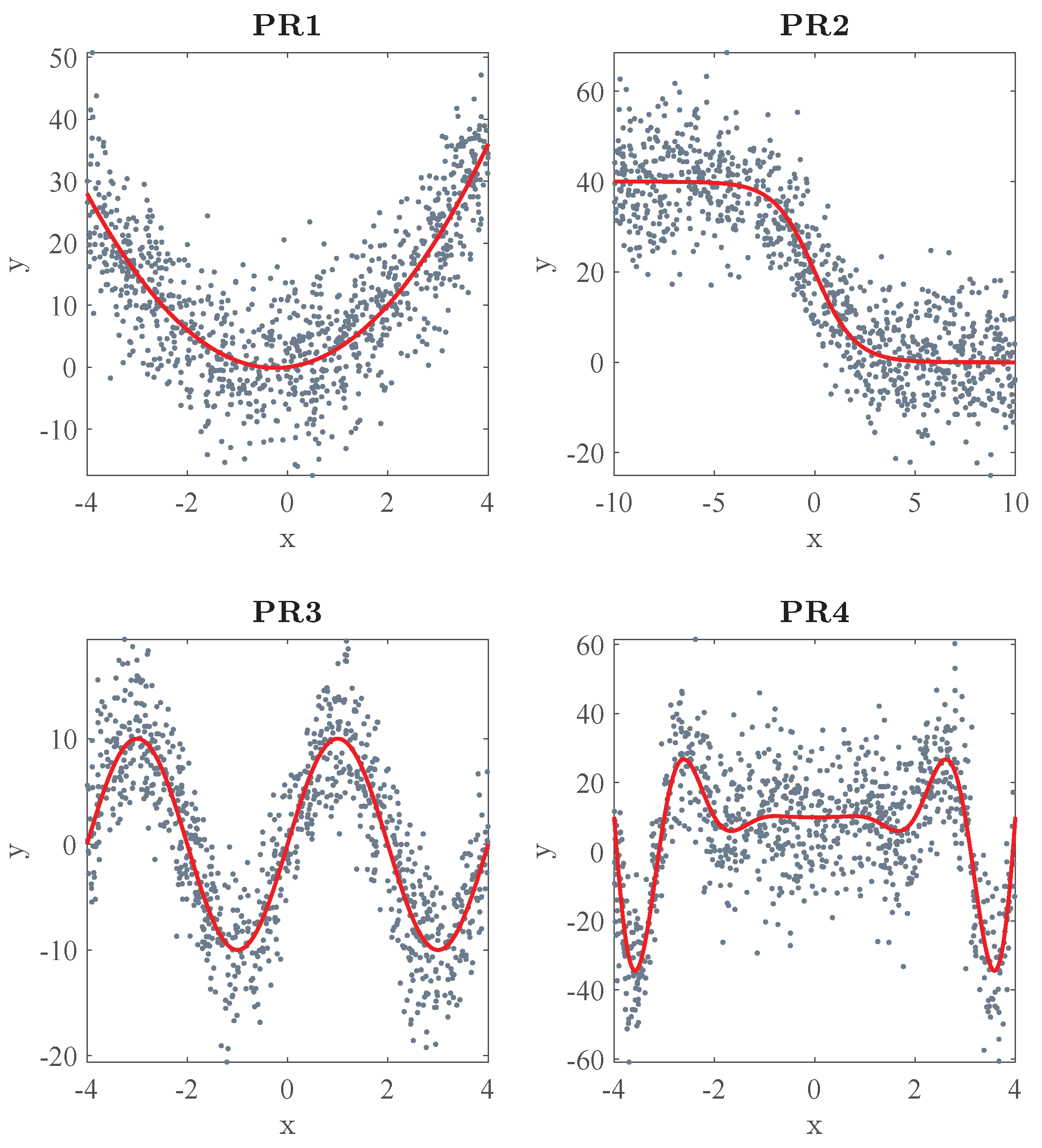
Figure 1. Continuous piecewise linear regression model. Top: Scattered data (N = 150 points) and fitted piecewise linear regression model, composed of K = 6 knots, plus and minus pointwise 99% standard error bands. Bottom: Set of six linear basis functions corresponding to the top model. The broken vertical lines indicate the x-positions of the knots.
Algorithms 17 00147 g001
Figure 2. Overall structure of all the considered methods.
Algorithms 17 00147 g002
Figure 3. Piecewise linear models: a set of 50 sub-models built with the LHM algorithm from 50 sub-samples (scattered data (n = 1000), representing one of them) and the true underlying function. The red ticks on the x-axis represent the positions of the knots.
Algorithms 17 00147 g003
Figure 4. Example of one iteration of the pruning algorithm: the p-value associated with each knot is calculated in this way, and the one with the highest value is removed. In this example, where only the standard error of two knots is plotted for simplicity, the knot j would be pruned.
Algorithms 17 00147 g004
Figure 5. Example of a complete pruning sequence of the method MC2. The zoom in the interest area shows how the elbow of the curve has been determined, and the selected K value.
Algorithms 17 00147 g005
Figure 6. Piecewise linear model obtained by combining the 50 sub-models (n = 1000) of Figure 3 using the MC3 method. The ticks on the x-axis represent the positions of the knots of all the sub-models (red) and the knots of the combined model (black), respectively.
Algorithms 17 00147 g006
Figure 7. Input datasets used in the simulations: scattered data (N = 1000) and true underlying functions of the problems shown in Table 1.
Algorithms 17 00147 g007
Figure 8. LHMs obtained in one replication using two different sample sizes: Problems PR1 (top) and PR4 (bottom), with datasets of N = 1 k (left) and N = 100 k (right). The black curve represents the true underlying function.
Algorithms 17 00147 g008
Figure 9. Distribution of K when varying the sample size N (calculated from 30 replications), for problems PR1 (top) and PR4 (bottom). For each N a compact boxplot shows the distribution of K. The red line connects their median values.
Algorithms 17 00147 g009
Figure 10. Distribution of the MSE when varying the sample size (calculated from 30 replications), for problems PR1 (top) and PR4 (bottom). For each N, three compact boxplots show the distribution of the MSE calculated over the SLS, STS, and TTS. A solid line shows the trend in each MSE. The black dashed line represents the true variance of the noise.
Algorithms 17 00147 g010
Figure 11. Bias–variance decomposition of the MSE(TTS) when varying the sample size N (calculated from 30 replications). Top: Problem PR1. Bottom: Problem PR4.
Algorithms 17 00147 g011
Figure 12. Impact of the parameters M and n on the accuracy of the combination models, and implications in terms of execution time and computing resources.
Algorithms 17 00147 g012
Figure 13. Comparison of the performance of the proposed methods when varying the sub-sample size (n) and the number of sub-samples (M) in the problem PR1 (calculated with 30 replications). Top: Distribution of the MSE over the TTS. Bottom: Distribution of the number of knots (K). The black dashed lines represent the 25th and 75th percentiles of the results obtained with the reference algorithm and a sample size of N = 10 M.
Algorithms 17 00147 g013
Figure 14. Comparison of the performance of the proposed methods varying the sub-sample size (n) and the number of sub-samples (M) in the problem PR4 (calculated with 30 replications). Top: Distribution of the MSE over the TTS. Bottom: Distribution of the number of knots (K). The black dashed lines represent the 25th and 75th percentiles of the results obtained with the reference algorithm and a sample size of N = 10 M.
Algorithms 17 00147 g014
Figure 15. Bias–variance decomposition of the MSE(TTS) of the proposed methods in the problem PR1. For each method: Top: Bias and variance varying n, with fixed M = 50. Bottom: Bias and variance varying M, with fixed n = 500 k. The background area represents the decomposition of the MSE(TTS) of the reference algorithm for this problem and a training dataset of N = 10 M.
Algorithms 17 00147 g015
Figure 16. Bias–variance decomposition of the MSE(TTS) of the proposed methods in problem PR4. For each method: Top: Bias and variance varying n, with fixed M = 50. Bottom: Bias and variance varying M, with fixed n = 500 k. The background area represents the decomposition of the MSE(TTS) of the reference algorithm for this problem and a training dataset of N = 10 M.
Algorithms 17 00147 g016
Figure 17. Comparison of the performance of the proposed methods in PR1, varying the number of sub-samples M (distributions calculated from 30 replications). Left: Small sub-sample size (n = 1 k). Right: Big sub-sample size (n = 1 M). Top: Distribution of the MSE over the TTS. Bottom: Distribution of the number of knots (K). The black dashed lines represent the 25th and 75th percentiles of the results obtained with the reference algorithm and a sample size of N = 10 M.
Algorithms 17 00147 g017
Figure 18. Comparison of the performance of the proposed methods in PR4, varying the number of sub-samples M (distributions calculated from 30 replications). Left: Small sub-sample size (n = 1 k). Right: Big sub-sample size (n = 1 M). Top: Distribution of the MSE over the TTS. Bottom: Distribution of the number of knots (K). The black dashed lines represent the 25th and 75th percentiles of the results obtained with the reference algorithm and a sample size of N = 10 M.
Algorithms 17 00147 g018
Figure 19. Bias–variance decomposition of the MSE(TTS) with and without a final OLS (calculated from 30 replications). The first two rows are related to PR1, and the other two are for PR4. Each column represents the results of a different method (MS, MC2, and MC3), with and without applying a final OLS. The background area represents the bias–variance decomposition of the MSE(TTS) obtained with the reference algorithm over a sample of size N = 10 M.
Algorithms 17 00147 g019
Table 1. Problem definition for testing the proposed methods.
ProblemTrue Function
PR1 f ( x ) = x + 2 x 2
PR2 f ( x ) = 40 / ( 1 + e x )
PR3 f ( x ) = 10 s i n ( ( π · x ) / 2 )
PR4 f ( x ) = 10 + x 3 · s i n ( π · x )
Table 2. Average MSE over the different datasets (SLS, STS, and TTS) in all the problems applying the proposed methods with different values of M and n = 1 M (calculated from 30 replications). Note that MS, MC2, and MC3 include a final OLS step. The last row represents the results of the reference algorithm (RA) using a sample of N = 10 M. The values with * represent the first value of M, for each problem and method, in which the error over the TTS is lower than the one obtained with RA. Values given in parentheses indicate the best method for each problem, obtained with minimum M.
PR1 (MSE)PR2 (MSE)PR3 (MSE)PR4 (MSE)
M SLS STS TTS SLS STS TTS SLS STS TTS SLS STS TTS
MS252.2252.27 1.31 × 10 2 63.9964.03 1.02 × 10 2 16.0016.00 3.31 × 10 3 149.71149.64 1.82 × 10 2
552.2252.27 1.11 × 10 2 63.9964.03 8.30 × 10 3 16.0016.00 3.28 × 10 3 149.71149.64 1.70 × 10 2
1052.2152.27 1.09 × 10 2 63.9964.03 7.77 × 10 3 16.0016.00 3.03 × 10 3 149.71149.64 1.73 × 10 2
2052.2252.27 1.10 × 10 2 63.9964.03 7.82 × 10 3 16.0016.00 3.04 × 10 3 149.71149.64 1.76 × 10 2
5052.2152.27 1.04 × 10 2 63.9964.03 7.09 × 10 3 16.0016.00 2.93 × 10 3 149.71149.63 1.72 × 10 2
MC1252.2152.27 9.02 × 10 3 63.9964.03 8.23 × 10 3 16.0016.00 2.74 × 10 3 149.70149.64 1.57 × 10 2
552.2152.26 5.41 × 10 3 63.9964.03 5.45 × 10 3 16.0016.00 1.98 × 10 3 149.70149.63 9.94 × 10 3
1052.2152.26 3.78 × 10 3 *63.9864.03 4.75 × 10 3 16.0016.00 1.73 × 10 3 149.70149.63 8.08 × 10 3
2052.2152.26 3.26 × 10 3 63.9864.03 4.24 × 10 3 16.0016.00 1.65 × 10 3 149.70149.63 7.29 × 10 3
5052.2152.26 3.09 × 10 3 63.9864.03 4.04 × 10 3 16.0016.00 1.56 × 10 3 149.70149.63 6.74 × 10 3
MC2252.2252.27 1.31 × 10 2 63.9964.03 1.23 × 10 2 16.0016.00 3.14 × 10 3 149.70149.64 1.53 × 10 2
552.2152.26 6.27 × 10 3 63.9864.03 5.14 × 10 3 16.0016.00 1.94 × 10 3 149.70149.63 9.55 × 10 3
1052.2152.26 3.13 × 10 3 *63.9864.02 3.60 × 10 3 16.0016.00 1.39 × 10 3 149.70149.63 7.84 × 10 3
2052.2152.26 1.84 × 10 3 63.9864.02 2.64 × 10 3 *16.0016.00 1.21 × 10 3 *149.70149.63 6.96 × 10 3 *
5052.2152.26 1.15 × 10 3 63.9864.02 1.73 × 10 3 16.0416.04 3.89 × 10 2 149.69149.63 5.77 × 10 3
MC3252.2152.26( 1.75 × 10 3 *)63.9864.02( 1.48 × 10 3 *)16.0016.00( 1.09 × 10 3 *)149.69149.63( 4.45 × 10 3 *)
552.2052.26 1.12 × 10 3 63.9864.02 1.06 × 10 3 16.0016.00 8.92 × 10 4 149.69149.63 4.89 × 10 3
1052.2052.26 9.26 × 10 4 63.9864.02 9.17 × 10 4 16.0016.00 7.97 × 10 4 149.69149.63 4.57 × 10 3
2052.2052.26 7.81 × 10 4 63.9864.02 8.46 × 10 4 16.0016.00 8.10 × 10 4 149.69149.63 4.23 × 10 3
5052.2052.26 7.09 × 10 4 63.9864.02 7.51 × 10 4 16.0016.00 7.21 × 10 4 149.69149.63 4.21 × 10 3
RA-52.2152.26 4.53 × 10 3 63.9864.02 2.86 × 10 3 16.0016.00 1.36 × 10 3 149.68149.63 7.06 × 10 3
Table 3. Bias–variance decomposition of the MSE(TTS) in all the problems applying the proposed methods with different values of M and n = 1 M (calculated from 30 replications). Note that MS, MC2, and MC3 include a final OLS step. The last row represents the results of the reference algorithm (RA) using a sample of N = 10 M.
PR1 (Bias–Var)PR2 (Bias–Var)PR3 (Bias–Var)PR4 (Bias–Var)
M Bias 2 Var Bias 2 Var Bias 2 Var Bias 2 Var
MS2 5.28 × 10 3 2.16 × 10 2 5.50 × 10 3 1.54 × 10 2 2.78 × 10 3 3.97 × 10 3 1.21 × 10 2 2.51 × 10 2
5 4.54 × 10 3 1.82 × 10 2 5.63 × 10 3 1.14 × 10 2 2.67 × 10 3 4.02 × 10 3 1.14 × 10 2 2.34 × 10 2
10 4.58 × 10 3 1.77 × 10 2 6.07 × 10 3 9.80 × 10 3 2.66 × 10 3 3.51 × 10 3 1.07 × 10 2 2.48 × 10 2
20 3.70 × 10 3 1.89 × 10 2 6.12 × 10 3 9.84 × 10 3 2.38 × 10 3 3.83 × 10 3 1.19 × 10 2 2.40 × 10 2
50 4.52 × 10 3 1.69 × 10 2 5.58 × 10 3 8.90 × 10 3 2.16 × 10 3 3.83 × 10 3 1.04 × 10 2 2.48 × 10 2
MC12 6.29 × 10 3 1.22 × 10 2 7.60 × 10 3 9.16 × 10 3 2.91 × 10 3 2.64 × 10 3 1.03 × 10 2 2.18 × 10 2
5 5.53 × 10 3 5.47 × 10 3 6.86 × 10 3 4.18 × 10 3 2.80 × 10 3 1.20 × 10 3 1.06 × 10 2 9.60 × 10 3
10 4.89 × 10 3 2.76 × 10 3 7.33 × 10 3 2.24 × 10 3 2.76 × 10 3 7.28 × 10 4 1.02 × 10 2 6.19 × 10 3
20 4.71 × 10 3 1.87 × 10 3 7.32 × 10 3 1.20 × 10 3 2.81 × 10 3 5.00 × 10 4 1.05 × 10 2 4.23 × 10 3
50 5.00 × 10 3 1.23 × 10 3 7.25 × 10 3 8.69 × 10 4 2.77 × 10 3 3.52 × 10 4 1.04 × 10 2 3.14 × 10 3
MC22 8.53 × 10 3 1.82 × 10 2 1.16 × 10 2 1.35 × 10 2 3.23 × 10 3 3.15 × 10 3 1.17 × 10 2 1.96 × 10 2
5 5.43 × 10 3 7.36 × 10 3 6.20 × 10 3 4.22 × 10 3 2.54 × 10 3 1.38 × 10 3 1.11 × 10 2 8.30 × 10 3
10 3.30 × 10 3 3.06 × 10 3 4.74 × 10 3 2.54 × 10 3 1.93 × 10 3 8.78 × 10 4 9.91 × 10 3 5.97 × 10 3
20 2.06 × 10 3 1.68 × 10 3 3.56 × 10 3 1.79 × 10 3 1.66 × 10 3 7.94 × 10 4 8.61 × 10 3 5.49 × 10 3
50 1.24 × 10 3 1.09 × 10 3 2.28 × 10 3 1.22 × 10 3 1.90 × 10 2 6.08 × 10 2 6.96 × 10 3 4.75 × 10 3
MC32 8.61 × 10 4 2.73 × 10 3 8.44 × 10 4 2.19 × 10 3 1.17 × 10 3 1.05 × 10 3 1.16 × 10 3 7.99 × 10 3
5 6.47 × 10 4 1.64 × 10 3 8.13 × 10 4 1.35 × 10 3 1.06 × 10 3 7.52 × 10 4 1.55 × 10 3 7.93 × 10 3
10 6.80 × 10 4 1.21 × 10 3 6.13 × 10 4 1.26 × 10 3 1.00 × 10 3 6.15 × 10 4 1.61 × 10 3 7.79 × 10 3
20 6.10 × 10 4 9.84 × 10 4 6.54 × 10 4 1.07 × 10 3 1.07 × 10 3 5.66 × 10 4 1.38 × 10 3 7.33 × 10 3
50 5.51 × 10 4 8.96 × 10 4 5.45 × 10 4 9.90 × 10 4 9.12 × 10 4 5.49 × 10 4 1.41 × 10 3 7.25 × 10 3
RA- 1.13 × 10 3 3.52 × 10 3 1.17 × 10 3 1.75 × 10 3 6.34 × 10 4 7.50 × 10 4 1.57 × 10 3 5.69 × 10 3
Table 4. Average CPU-time of the proposed methods with different values of M and n = 1 M, applied to all the problems (calculated from 30 replications). tsub represents the total calculation time of the sub-models. tsc represents the execution time of the model selection or combination method. This time includes a final OLS in the case of MS, MC2, and MC3. ttot shows the total execution time. The last row represents the results of the reference algorithm (RA) using a sample of N = 10 M.
PR1 (Time (s))PR2 (Time (s))PR3 (Time (s))PR4 (Time (s))
M t sub t sc t tot t sub t sc t tot t sub t sc t tot t sub t sc t tot
MS218.553.4421.9916.383.0919.4722.346.8329.1733.399.5642.95
554.873.5458.4146.873.1850.0561.546.8368.3795.329.57104.89
10138.563.55142.11117.973.16121.13151.436.82158.26224.609.51234.11
20283.713.58287.28245.993.18249.17311.646.74318.39455.199.42464.61
50788.093.58791.67662.483.23665.71797.616.79804.401156.449.521165.95
MC1218.550.0018.5516.380.0016.3822.340.0022.3433.390.0033.39
554.870.0054.8746.870.0046.8761.540.0061.5495.320.0095.32
10138.560.00138.57117.970.00117.97151.430.00151.44224.600.00224.60
20283.710.01283.72245.990.01246.00311.640.01311.65455.190.01455.20
50788.090.02788.11662.480.02662.49797.610.02797.621156.440.021156.45
MC2218.558.6127.1516.387.6724.0522.3417.2739.6133.3922.5555.94
554.8711.3066.1746.8710.4757.3561.5423.1984.7295.3228.90124.22
10138.5613.51152.07117.9711.79129.75151.4327.04178.47224.6031.94256.54
20283.7110.48294.19245.998.65254.64311.6421.24332.89455.1926.53481.72
50788.0918.35806.44662.4815.42677.90797.6133.59831.201156.4444.881201.32
MC3218.5529.1247.6616.3826.7943.1722.3453.2475.5833.3988.24121.63
554.8731.0385.9046.8727.4374.3061.5453.33114.8795.3288.01183.34
10138.5632.21170.77117.9727.64145.61151.4352.19203.62224.6084.47309.07
20283.7121.29304.99245.9917.24263.23311.6435.61347.26455.1960.57515.76
50788.0931.87819.96662.4827.52689.99797.6150.69848.301156.4482.851239.29
RA---114.87--83.82--147.19--180.37
Disclaimer/Publisher’s Note: The statements, opinions and data contained in all publications are solely those of the individual author(s) and contributor(s) and not of MDPI and/or the editor(s). MDPI and/or the editor(s) disclaim responsibility for any injury to people or property resulting from any ideas, methods, instructions or products referred to in the content.

