Abstract
Reinforcement learning is an important technique in various fields, particularly in automated machine learning for reinforcement learning (AutoRL). The integration of transfer learning (TL) with AutoRL in combinatorial optimization is an area that requires further research. This paper employs both AutoRL and TL to effectively tackle combinatorial optimization challenges, specifically the asymmetric traveling salesman problem (ATSP) and the sequential ordering problem (SOP). A statistical analysis was conducted to assess the impact of TL on the aforementioned problems. Furthermore, the Auto_TL_RL algorithm was introduced as a novel contribution, combining the AutoRL and TL methodologies. Empirical findings strongly support the effectiveness of this integration, resulting in solutions that were significantly more efficient than conventional techniques, with an 85.7% improvement in the preliminary analysis results. Additionally, the computational time was reduced in 13 instances (i.e., in 92.8% of the simulated problems). The TL-integrated model outperformed the optimal benchmarks, demonstrating its superior convergence. The Auto_TL_RL algorithm design allows for smooth transitions between the ATSP and SOP domains. In a comprehensive evaluation, Auto_TL_RL significantly outperformed traditional methodologies in 78% of the instances analyzed.
1. Introduction
Reinforcement learning (RL) brings together important machine learning (ML) methods [1,2,3,4,5,6,7,8,9]. With RL, an agent learns from interaction with the environment [3,4]. Also, RL is based on Markov decision processes (MDP), and the goal is to maximize the reward received over time [3,4].
A recent field of research studied in association with RL is automated machine learning (AutoML). When AutoML is applied to RL, the approach is called automated reinforcement learning (AutoRL) [10]. AutoRL is an intelligent system designed to select the appropriate conditions for reinforcement learning before learning begins [11]. The use of AutoRL aims to reduce the need for knowledge required by the user as well as reduce the computational cost required during learning [11,12]. These initial conditions can be defined through metalearning, in which the system will use its previous experiences to carry out future activities [12,13,14,15,16].
One way of improving AutoRL approaches is through the use of transfer learning (TL). TL aims to accelerate learning by providing autonomy to the system [17]. The purpose is to transfer knowledge between tasks in different domains and provide various benefits, such as improving the performance of the agent in the target task, improving the agent’s total reward and reducing the time needed to carry out the learning [17,18]. Along these lines, transfer reinforcement learning techniques have been applied in important domains, especially in the areas of robotics [19,20,21,22,23,24] and multiagent systems [25,26,27]. However, the literature has paid little attention to the transfer reinforcement learning for combinatorial optimization problems.
Indeed, the field of combinatorial optimization has several studies using RL [6,28,29,30,31,32,33,34]. Some domains with applications of RL techniques are the traveling salesman problem (TSP) [29,31], k-server problem [32,34], multidimensional knapsack problem [35], vehicle routing [36] and sequential ordering problem (SOP) [37].
The TSP [29,31,33] and the SOP [38,39,40,41] are problems that have great relevance in the literature, which has led to several studies on them. The TSP is a problem with numerous relevant applications, and as a result, several studies have been carried out to solve it [42,43,44,45]. The SOP, like the TSP, also has several important studies, including energy optimization in compilers [46], search optimization [39,47] and parallel machine scaling [48]. Moreover, the TSP and SOP are NP-hard combinatorial optimization problems; that is, in practice, it is necessary to adopt approximate algorithms in the search for better solutions [39]. However, the literature still lacks studies that address tranfer RL in these two problems.
Therefore, the goal of this work is to propose and analyze transfer reinforcement learning between these two relevant combinatorial optimization domains: the ATSP and SOP. For this purpose, instances of the TSPLIB library [49,50,51] and the state–action–reward–state–action (SARSA) algorithm [4] were used. The approach proposed in this work enables generation of a knowledge base in the source domain (ATSP) to transfer learning to the target domain (SOP). In addition to the extensive variety of studies on the ATSP and SOP, these domains were selected due to the similarities in the characteristics of these two combinatorial optimization problems. In this sense, in this paper, three criteria are proposed to be evaluated when carrying out transfer reinforcement learning across combinatorial optimization problems: (1) problems with the same objective function; (2) similar datasets; and (3) transfer from the simpler domain to the more complex domain.
The main contributions include the following:
- A transfer reinforcement learning approach between two classical combinatorial optimization problems. The asymmetric traveling salesman problem is the source domain, and the sequential ordering problem is the objective domain.
- Apply transfer learning to these problems and statistically analyze the results obtained with the transfer.
- Develop a new AutoRL algorithm, apply it to the problems studied and analyze its results.
The present paper is organized into six sections. Section 2 defines the theoretical aspects of the combinatorial optimization problems adopted, RL, AutoML and transfer learning. Section 3 and Section 4 present the methodology and results, respectively. Section 5 shows the comparison of this paper with other literature studies. Finally, Section 6 presents the conclusions of the work.
2. Background
This section will discuss the topics of reinforcement learning, combinatorial optimization, the traveling salesman problem, the SOP, automated machine learning and finally, the transfer learning technique.
2.1. Reinforcement Learning
Reinforcement learning is based on Markov decision processes [3,4]. An MDP is structured into a finite set of states (S), a finite set of actions (A), a finite set of reinforcements (R) and a state transition model (T) [3,4].
In RL, an agent learns through trial and error to make decisions in an environment. Basically, the learning agent performs a sequence of three steps in several repetitions:
- (i)
- Perceive the current state (s);
- (ii)
- Perform an action (a);
- (iii)
- Receive a reward ().
In addition, at each instant of time (t), a learning matrix (Q) is updated which stores the knowledge learned. This Q matrix has the dimension given by the number of states in relation to the number of actions in the model.
Equation (1) presents the method for updating the Q matrix using the SARSA algorithm [4]:
where s is the state, a the action at time t, is the reward for executing a in s, is the new state, is the new action selected, and are matrices at the current time and at , respectively, is the learning rate and is the discount factor.
Algorithm 1 represents the SARSA algorithm [4].
| Algorithm 1: SARSA algorithm | |
| 1 | Set the parameters: |
| 2 | In each s,a do Q(s,a) = 0 |
| 3 | Observe the state s |
| 4 | Select action a using policy -greedy |
| 5 | do |
| 6 | Run the action a |
| 7 | Receive the immediate reward r(s,a) |
| 8 | Observe the new state s′ |
| 9 | Select action a′ using policy -greedy |
| 10 | |
| 11 | s = s′ |
| 12 | a = a′ |
| 13 | while the stop criterion is satisfied; |
In Algorithm 1, the - [4] action selection policy is adopted. This method uses the parameter to control gluttony and randomness in decision making. For example, if , then the system will select random actions in of the cases and the best-estimated actions for each state in the learning matrix in of the situations.
2.2. Combinatorial Optimization
Combinatorial optimization problems aim to maximize or minimize an objective function defined in a certain finite domain that classifies the solution to the problem as optimal [52,53]. Briefly, these problems can be characterized as follows [53,54,55]:
- Decision variables are the criteria that will be manipulated in the search for the optimal solution.
- The objective function is the function that contains the decision variables that will be altered during the search for the best solution to the problem. It should be noted that every combinatorial optimization issue has at least one objective function.
- Restrictions are conditions imposed on the problem to ensure that the solution found is feasible. It is important to note that it is not mandatory for a problem to have constraints, in which case all solutions are considered feasible.
The literature contains various optimization problems, including the following [52,55,56]:
- The traveling salesman problem;
- The knapsack problem;
- The sequential ordering problem;
- The quadratic assignment problem.
2.3. Traveling Salesman Problem
The traveling salesman problem is one of the best-known combinatorial optimization problems [57]. This method aims to determine a Hamiltonian cycle that passes through all the vertices of a graph. In addition, the problem also aims for the Hamiltonian cycle found to be the one with the lowest cost [52,57,58].
The TSP is made up of a set of cities, where the cashier must visit all the cities in the set, and at the end of the journey, the cashier must return to the initial city. As a restriction, each city in the set must be visited only once, except for the final city, which must be the same as the starting city [57,58].
The TSP can be classified in various ways, including the symmetrical TSP and asymmetrical TSP. In the symmetrical TSP, the cost of moving from node A to node B is the same as the cost of moving from node B to node A. In the case of the asymmetric TSP, the cost varies according to the direction of travel adopted [57]. Thus, the symmetric TSP can be represented by a graph with bidirectional edges, while the asymmetric TSP can be represented by a graph with directional edges [57].
The traveling salesman problem has several applications, and the authors of [52,58] presented some of them:
- Task sequencing;
- Drilling printed circuit boards;
- Analysis of crystal structures;
- Handling of stock items;
- Optimizing the movement of cutting tools;
- Postal delivery routing.
Formulation
There are several possible formulations for the TSP, some of which are presented in [52,59]. The following formulation was presented in [59] in Equations (2)–(6):
subject to
The objective function of the TSP is represented by Equation (2), in which represents the cost between cities i and j, and represents whether the arc (i, j) is part of the solution to the problem. If is equal to one, then the arc is part of the solution. If equals zero, then the arc is not part of the solution. In addition, Equations (3) and (4) ensure that each city will only be visited once. Equation (5), on the other hand, represents the restriction that the value of will always be binary. Finally, Equation (6) guarantees that no sub-routes will be formed when solving the problem [58,59].
2.4. Sequential Ordering Problem
The sequential ordering problem is an NP-hard combinatorial optimization problem and a variation of the asymmetric traveling salesman problem (ATSP), with the addition of precedence constraints [39,47]. Thus, as with the asymmetric TSP, the SOP also aims to find a Hamiltonian cycle of a minimum cost in a directed graph [39]. Thus, the search for the optimal solution to this problem becomes impractical, resulting in the need to apply algorithms to find the best approximate solutions [39].
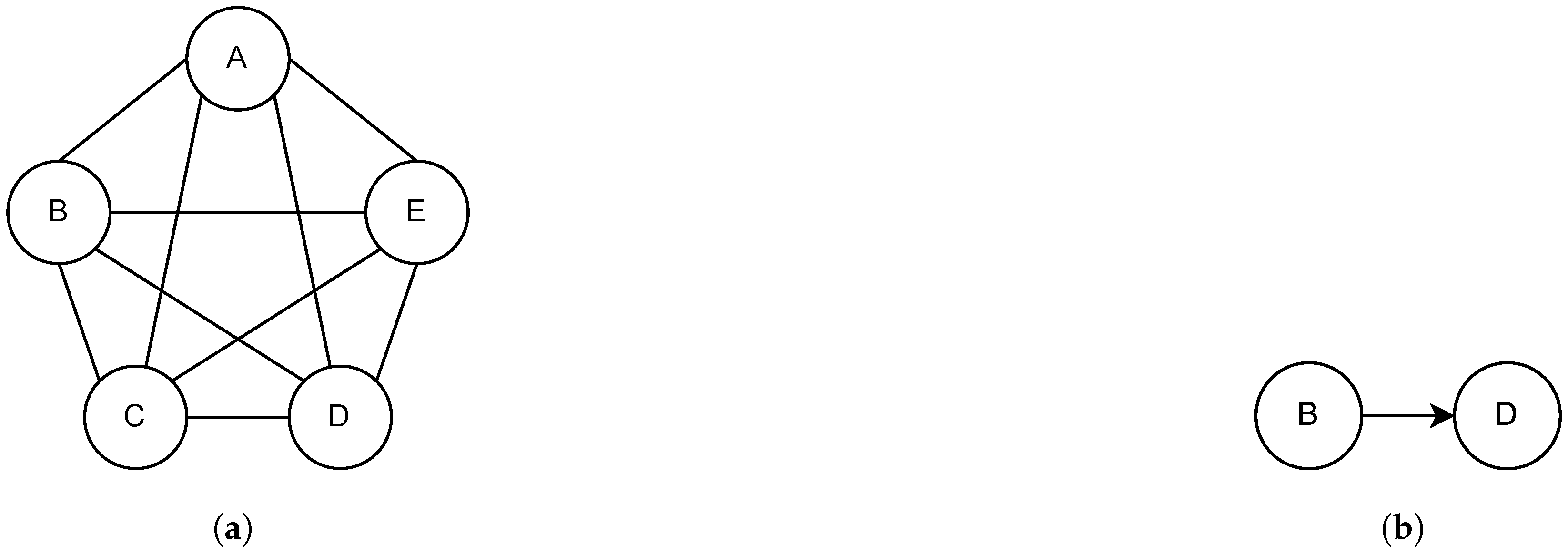
Consider that Figure 1 is a representation of an SOP problem. In this case, Figure 1a shows the graph that depicts this problem. Figure 1b shows the constraints of this problem. Assuming that the agent starts its trajectory at vertex A, according to the problem constraint, some valid routes are or . On the other hand, routes and are some invalid routes, as they do not respect the problem’s precedence restriction.
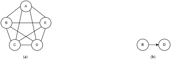
Figure 1.
Example of SOP problem representation and its constraint. (a) SOP problem diagram. (b) Problem precedence constraint.
In the SOP, also represents the cost of the arc. When , this value will represent the cost of moving from city i to city j. When , this value indicates that there is a precedence constraint. In this case, city j must precede city i [39].
In [37], the authors presented a formulation for the SOP based on the TSP formulation in [59]. This adds the following restriction to the TSP formulation presented previously, according to Equation (7):
This new constraint aims to satisfy the existing order of precedence restriction in the SOP.
2.5. Automated Machine Learning
Automated machine learning was developed with the main aim of reducing the human effort required when adjusting the learning settings [60,61]. Thus, AutoML is a technique used to define the parameters and algorithms that will be adopted during learning in order to obtain better results, given that the settings will be made according to the problem being studied [62,63].
In this context, due to the improvements observed through the use of AutoML and the growing need for increasingly robust learning systems, in order to cope with the abundance of data that is constantly emerging, this technique has also been used to automate other stages of the learning process [60,63,64].
Metalearning is one of the topics related to AutoML and refers to the system’s ability to learn how to learn [12,65,66]. In this sense, the goal of metalearning is to reuse previous experiences in tasks that will be performed in the future [12,13,65]. In this way, the system does not have to learn from scratch and can adapt to the current situation based on its previous experiences [67]. Therefore, there will be a reduction in the effort used to carry out the next tasks compared with the effort used to carry out the previous tasks [12,68]. It is worth noting that the greater the similarity between the tasks (the tasks already carried out and the tasks to be carried out), the greater the chances of obtaining good results by reusing knowledge obtained in previous tasks [14,68].
2.6. Transfer Learning
The main idea of transfer learning techniques is to use the knowledge that has already been acquired (tasks that have already been carried out) in related problems [17,26,69]. In this sense, some objectives of TL methods are to improve performance and reduce the time needed to learn a complex task [17].
For transfer learning, the knowledge base is first generated in a source domain and then applied to the target domain [17,18]. This approach is extremely beneficial in various situations, particularly when training for the target problem is complex [70]. By conducting experiments on a source problem, knowledge can be transferred to the target problem.
There are several possible applications for TL, some of which involve the following:
- Image analysis [71,72,73];
- Pattern recognition [74];
- Optimization problems [75].
One method for transfer reinforcement learning involves directly transferring the learning matrix Q as described in [18]. This method adopts the Q values from the source task as the starting point for the learning matrix in the objective domain. Equation (8) represents the direct transfer of RL between domains [18]:
3. Methodology
The transfer learning approach proposed in this paper aims to improve the performance of RL algorithms for solving combinatorial optimization problems. For this, concepts from the meta-learning research field were adopted [12]. Initially, the application of representational transfer stands out, which refers to the training of source and target models at different times; in other words, metaknowledge is transferred based on previous experience acquired. The second concept is the search for similarities in characteristics between datasets in order to improve the performance of learning algorithms. Thus, transfer of knowledge across tasks is an area of meta-learning that seeks to explore the experience obtained in previously learned datasets, domes or problems.
Following this line, this paper proposes three topics to be evaluated when performing transfer RL between combinatorial optimization problems:
- Problems with the same objective function: The objective function is a main characteristic of the mathematical modeling of a combinatorial optimization problem. This was a relevant criterion in deciding the two problems evaluated in this paper (the ATSP and SOP), considering that both aim to minimize the distance of a route.
- Similar datasets: The similarity between datasets can be assessed through the analysis of metafeatures, such as by performing descriptive statistics [12]. In this paper, the simulated domains have instances in the TSPLIB library. Furthermore, the instances selected for the target problem (SOP) originate from the source domain (ATSP), adding some variations such as precedence restrictions. These characteristics reinforce the similarities across the evaluated datasets.
- Transfer from the simpler domain to the more complex domain: This point reflects the relevance of decreasing the computational cost in the objective problem while promoting accelerated learning and advancing performance in the best solution. In this paper, the ATSP is the source domain (simplest), and the SOP is the objective domain (more complex), as the second problem adds precedence restrictions.
In sequence, this section describes in detail the methodology adopted to carry out this work. Initially, the dataset was built from the library TSPLIB (http://comopt.ifi.uni-heidelberg.de/software/TSPLIB95/, accessed on 1 December 2023). In this context, the specific problems to be investigated and their respective instances were selected. A model based on reinforcement learning was then developed, using the SARSA algorithm to tackle combinatorial optimization problems. As for the application of the transfer learning technique, the strategy was outlined in three phases: the construction of the knowledge base, the execution of the necessary experiments and the formulation of the methodology for analysis. Finally, an automated reinforcement transfer learning algorithm was created and structured in two stages: proposing an algorithm called Auto_TL_RL and carrying out practical experiments to validate and evaluate the algorithm.
3.1. Dataset
The TSPLIB [49] library is a data repository with instances for case studies of combinatorial optimization problems. TSPLIB is frequently adopted in the literature [30,31,37,39,41], and therefore, it was selected for this paper. Among the data available in the repository are data from problems such as the following [50]:
- The symmetric traveling salesman problem: the cost of traveling between two nodes is the same, regardless of the direction of travel;
- The asymmetric traveling salesman problem: the cost of traveling between two nodes depends on the direction of travel;
- The sequential ordering problem: this problem has precedence restrictions and also considers that the cost of traveling between two nodes depends on the direction adopted for travel.
The instances selected for use in the experiments are shown in Table 1 (ATSP) and Table 2 (SOP). These tables have three columns: problem, nodes and optimal:

Table 1.
ATSP instances.
Table 2.
SOP instances.
- Problem: instance name;
- Nodes: number of nodes in the problem;
- Best known solution: the best known value presented by TSPLIB.
To exemplify the data on the adopted instances, Table 3 and Table 4 present instances br17 (ATSP) and br17.12 (SOP), respectively.
Table 3.
Example of ATSP instance br17 (TSPLIB).
Table 4.
Example of SOP instance br17.12 (TSPLIB).
Table 3 and Table 4 reveal some characteristics of the data matrices adopted in this paper. Initially, it is worth highlighting that the values in the matrix cells represent the weights between vertices. For example, looking at the first row and second column of Table 3, is equal to three, as it represents the weight of traveling from to . It was also observed that the dimension of the matrix revealed the number of nodes in the instance. In this sense, br17 had a dimension of 17 (Table 3), while br17.12 had a dimension of 18 (Table 4). This relationship shows that the SOP instances had dimensions of in relation to the corresponding ATSP instances, where N is the dimension of the ATSP instance. Note also the changes made to Table 4 in relation to Table 4, where some data positions were replaced with the value “”, indicating the addition of a precedence constraint. For example, in the second row and fifth column in Table 3, the value is . On the other hand, in Table 4, this value was changed to “”, becoming an SOP precedence restriction.
3.2. Reinforcement Learning Model
The RL system developed was designed to apply the SARSA algorithm to experiments with combinatorial optimization problems: the ATSP and SOP. For this purpose, the model structure (actions, states and reinforcements) was adopted based on works in the literature [29,30,31,37,76]:
- States are the locations that must be visited to form the route. Thus, the number of states varies according to the number of nodes (N) in the instance.
- Actions represent the possible movements between locations (states). The initial number of actions is equivalent to the number of states in the model. However, the actions available for execution vary according to the cities already visited when developing the route.
- Reinforcements are the cost of travel () between the departure city (i) and the destination city (j), given as a function of the cost of travel (). The greater the distance between the nodes, the more negative the reinforcement will be, according to Equation (9):
Also, the RLSOP algorithm [37] was adopted to deal with the precedence restrictions of the SOP. The RLSOP (Algorithm 2) checks whether the actions (arrival location) selected by the - method have precedence restrictions. If this is the case, then another destination is selected and checked again.
| Algorithm 2: Algorithm for analyzing precedence restrictions in the selection of actions from RL to SOP (RLSOP) [37] | |
| 1 | a_t = e-greedy(); |
| 2 | cont = 0; |
| 3 | while cont == 0 do |
| 4 | if there are precedence restrictions for the selected action then |
| 5 | if at least one action corresponding to the precedence constraints of a_t has not yet been selected then |
| 6 | cont = 0; |
| 7 | else |
| 8 | cont = 1; |
| 9 | end |
| 10 | end |
| 11 | if cont == 0 then |
| 12 | remove the action a_t from the list of available actions at time t; |
| 13 | a_t = e-greedy(); |
| 14 | end |
| 15 | end |
| 16 | Return to_t; |
3.3. Transfer Learning Approach
To implement the transfer learning technique, it is necessary to follow three steps:
- Generation of the knowledge base;
- Experiments for transfer learning;
- Elaboration of the methodology for analysis.
3.3.1. Generation of the Knowledge Base
The knowledge base generation stage was conducted through experiments with TSPLIB instances of the asymmetric traveling salesman problem. Among the instances shown in Table 1, the following ATSP instances were selected for use in this approach: br17, p43, ft53 and kro124p. SOP instances derived from the selected ATSP instances were also used (Table 2).
The experiments with each of the four ATSP instances were configured with 10,000 episodes, where one episode is equivalent to a complete route between the nodes. The learning matrix in these simulations was initialized with zeros. In addition, the parameters were set to , and , based on the results in [37,76].
At the end of each simulation, the final learning matrix (QATSP) was stored. In this sense, four QATSP matrices were generated, with one per ATSP instance (br17, p43, ft53 and kro124p). This knowledge base was adopted in the transfer learning experiments for the SOP domain, which are explained in the next subsection.
3.3.2. Experiments for Transfer Learning
In this phase, experiments were carried out to assess the influence of knowledge transfer between the ATSP (source) and SOP (goal) domains. Table 5 shows the 14 SOP instances adopted in this stage, as well as their respective optimal values, number of nodes and precedence restrictions.
Table 5.
SOP problems adopted and respective numbers of nodes, precedence constraints and best known solution values according to TSPLIB. The number of constraints refers to the number of values of in the instance.
Experiments were carried out using two initial conditions for the learning matrix (Q):
- Q0, meaning without transfer learning. The learning matrix was initialized with all null values.
- The QATSP, adopting the knowledge base generated from the experiments with the source domain (ATSP).
In order to use the knowledge base (QATSP), adjustments had to be made to the original learning matrices (experiments with the ATSP). The reason for this is that the state spaces of the ATSP and SOP domains are different. For example, the kro124p instance (ATSP source) has 100 nodes, while the equivalent SOP problems contain locations: kro124.p1, kro124.p2, kro124.p3 and kro124.p4. Thus, a row and a column (with zeros) were added to the QATSP knowledge base matrices for use by the SOP domain.
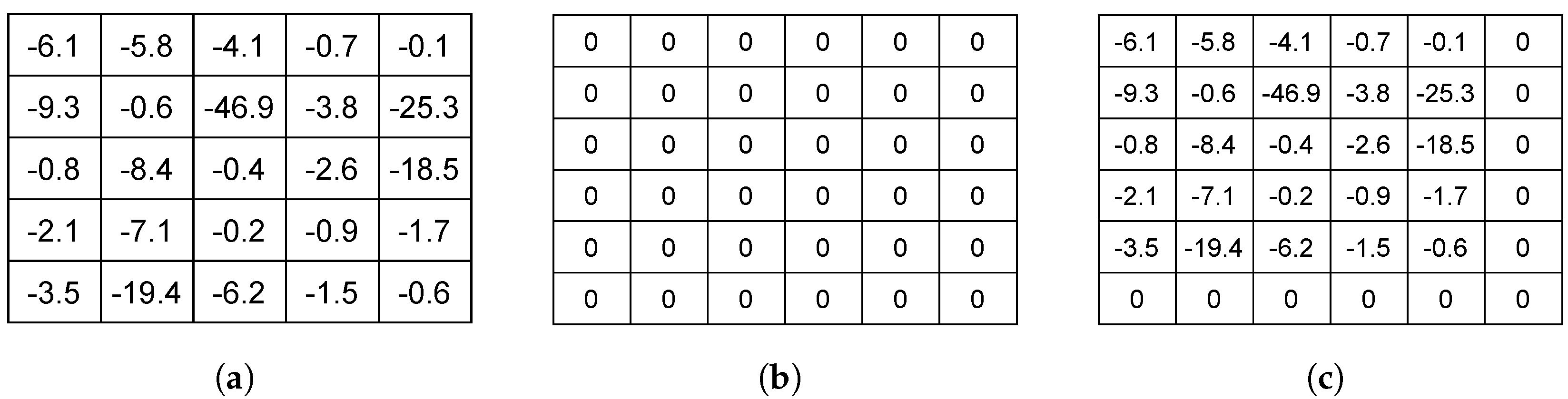
Figure 2 illustrates how the transfer RL process takes place. Normally, during experiments, the learning matrix is initialized with zeros (Figure 2b). Assuming that Figure 2a shows the learning matrix of an ATSP instance at the end of the experiment, with the proposed learning transfer approach, the experiment learning matrix of an SOP instance would initially be filled in as shown in Figure 2c.
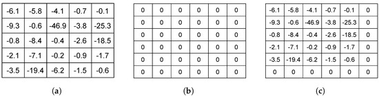
Figure 2.
Example of the transfer RL process. (a) ATSP instance learning matrix. (b) SOP instance learning matrix without transfer learning. (c) SOP instance learning matrix with transfer learning.
The experiments with each of the SOP problems and initial conditions (Q0 and QATSP) were run with 100 episodes in 10 epochs (repetitions). It is worth noting that only 100 episodes were used in this stage, as the goal was to analyze the adoption of transfer learning as a method to accelerate RL in the objective domain [17]. In this way, the aim was to assess whether the adoption of the knowledge base (QATSP) reproduced good results in a few episodes of SOP simulation.
The parameters for this stage were defined in the same way as in the previous section: , and .
3.3.3. Analysis Methodology
The analysis methodology proposed in this paper has three stages. This methodology was based on metrics found in the literature [17,26]:
- (i)
- Preliminary analysis;
- (ii)
- Computational time analysis;
- (iii)
- Results visualization and interpretation.
The preliminary analysis compares the average results achieved in the SOP instances with and without transfer learning from the source domain (ATSP). This metric is similar to the “total reward” [17], which adopts the total reinforcement received by the agent during learning.
The second stage aims to evaluate the differences between the computational times of the simulations with Q0 and the QATSP. According to [17], one possible goal of transferring knowledge between domains is to reduce the time it takes to learn a complex task.
In these first two steps, the t test is used to compare the means of two independent samples. This statistical method assesses whether two population means ( and ) are statistically equal or different [77] through the following hypotheses:
Adopting a significance level of 5%, the decision rule is as follows. If , then the means are considered to be statistically equal. On the other hand, when , the means are concluded to be statistically different. To validate the results, it is necessary to test the normality assumption for each of the independent samples. In this study, the Kolmogorov–Smirnov (KS) test was adopted [78], where the normality assumption was satisfied as long as the p value of this test was greater than 5%. Thus, after verifying that the assumptions were guaranteed by the KS test for all the samples, the t test was applied to compare the average results for the distance on the route (preliminary analysis) and computational time for each of the 14 simulated instances.
Finally, results visualization and interpretation evaluates the learning curves of the following SOP instances: krop124p.1, krop124p.2, krop124p.3 and krop124p.4. Three metrics were analyzed: the distance calculated in the first episode (), the distance in the last episode () and the smallest solution found (). Evaluating the solution of the first (“jump start”) and last (“asymptotic performance”) episodes was important for seeing the difference in the results of Q0 and the QATSP in these situations [17]. The value of , on the other hand, allowed us to compare whether adopting a knowledge base (QATSP) led to better solutions.
3.4. Automated Transfer Reinforcement Learning Method
This section introduces the automated reinforcement learning transfer method, which aims to automate the transfer of reinforcement learning between the ATSP and SOP problems. The method consists of two stages:
- A new automated transfer reinforcement learning algorithm (Auto_TL_RL).
- Automated transfer reinforcement learning experiments.
3.4.1. Automated Transfer Reinforcement Learning Algorithm (Auto_TL_RL)
The flowchart depicted in Figure 3 illustrates the proposed automated transfer reinforcement learning algorithm flow, which has been named Auto_TL_RL. Initially, an SOP instance is selected, and if a knowledge base already exists for the selected SOP instance, then the problem is executed directly. Otherwise, the knowledge base is generated from an ATSP instance, this database is then stored, and finally the SOP is executed.
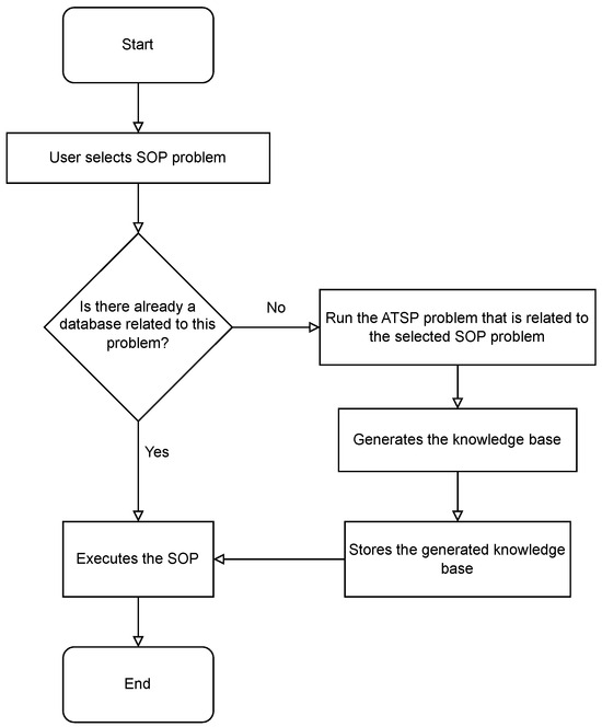
Figure 3.
Flowchart showing how the proposed Auto_TL_RL algorithm works.
Algorithm 3 represents the proposed Auto_TL_RL algorithm procedurally, which was developed using the R language. It is worth noting that the proposed algorithm uses the SARSA algorithm to perform the ATSP and SOP.
| Algorithm 3: Auto_TL_RL Algorithm | |
| 1 | Specify the SOP instance to be executed |
| 2 | Extract the size of the SOP instance |
| 3 | Set the parameter: |
| 4 | Set the number of episodes: 1000 |
| Stage 1 | |
| 5 | Checking the existence of the knowledge base |
| Stage 2 | |
| 6 | Specify the ATSP instance that will be executed |
| 7 | Extract the size of the ATSP instance |
| 8 | Set the parameters: and |
| 9 | Set the number of epochs: 5 |
| 10 | foreach ∈ do |
| 11 | foreach ∈ do |
| 12 | for epoch to numberEpochs do |
| 13 | SARSA(, , sizeOfInstance) |
| 14 | end |
| 15 | end |
| 16 | end |
| 17 | Stores the database generated |
| Stage 3 | |
| 18 | Set the parameters: and |
| 19 | Set the number of epochs: 10 |
| 20 | for epoch to numberEpochs do |
| 21 | SARSA(, , sizeOfInstance) |
| 22 | end |
Initially, the user must select the instance of the SOP to execute (line 1), and from this, the size of the instance is extracted (line 2). Next, the value of the -greedy parameter and the number of episodes that will be executed during learning must be defined (lines 3 and 4). Next, the execution of the algorithm is divided into three stages. The first stage checks for the existence of the database related to the selected problem (line 5). To check for the existence of the knowledge base, a document is used that records the name of the instance, the dimension, the status of the knowledge base (whether it exists or not) and the name of the file that stores the knowledge base corresponding to the instance analyzed.
The second path is taken if there is no pre-existing knowledge base for the selected SOP instance. It defines an ATSP instance and extracts its dimension (lines 6 and 7). Furthermore, the values for the learning rate, the discount factor and the number of epochs are defined (lines 8 and 9). In this sense, with the learning rate and discount factor values defined, different parameter combinations are performed. For each simulated parameter combination, the selected ATSP instance is executed for the defined number of epochs (lines 10–16). At the end of the execution, the knowledge base that resulted in the shortest route distance in the ATSP instance used is stored among all generated databases (line 17), allowing it to be reused in future applications. Finally, in the third step, the SOP is executed (lines 18–22) using the knowledge base generated in the previous step.
The second path is adopted when there is no pre-existing knowledge base for the selected SOP instance. Thus, an ATSP instance is defined, and its dimension is extracted (lines 6 and 7). Furthermore, the values for the learning rate, discount factor and number of epochs are defined (lines 8 and 9). In this sense, with the learning rate and discount factor values established, various combinations of parameters are performed. For each simulated parameter combination, the selected ATSP instance is executed for the defined number of epochs (lines 10–16). At the end of the execution, the knowledge base that resulted in the shortest route distance in the ATSP instance used is stored among all generated databases (line 17), allowing it to be reused in future applications. Finally, the third stage is where the SOP is executed (lines 18–22) using the knowledge base generated in the previous step.
The Auto_TL_RL algorithm in R language has been made available in an open repository to provide detailed visualization of the technical aspects of the code and to ensure its reproducibility (https://github.com/KellyBarbosa/auto_tl_rl, accessed on 12 February 2024).
3.4.2. Automated Transfer Reinforcement Learning Experiments
Automated transfer reinforcement learning experiments were also performed using SOP and ATSP instances provided by the TSPLIB library. The selected ATSP and SOP instances are shown in Table 1 and Table 2, respectively. In this approach, the following ATSP instances were selected: br17, p43, ry48p, ft53 and ft70. In addition to the ATSP problems, the SOP instances that were derived from the selected ATSP instances were also selected.
The parameters, number of epochs and number of episodes to be used in the proposed Auto_TL_RL algorithm (Algorithm 3) during the experiments were also defined. The configurations for the second stage were the same as those presented in [79], and they can be seen in Table 6. The learning conditions for the final stage followed the same structure. However, some adaptations were made to better suit the experimental scenarios, as shown in Table 7.
Table 6.
Configurations used during the second stage of the experiment.
Table 7.
Configurations used during the third stage of the experiment.
4. Results
This section presents the results of the preliminary analysis and the automated transfer learning experiments.
4.1. Results of Preliminary Analysis
For a more comprehensive understanding, the results of the preliminary analysis are presented and detailed in three separate sections: Preliminary Analysis, Computational Time Analysis, Results Visualization and Interpretation.
4.1.1. Preliminary Analysis
The preliminary analysis compares the solutions (distance on the route) according to the initial learning condition adopted (Q0 or the QATSP). For each instance, the average solution of the 10 simulated repetitions was calculated. Table 8 shows the results of this stage.
Table 8.
Average solution (distance) over the course of learning to solve the SOP, percentage difference (D) between the results of Q0 and the QATSP and results of the t test. There was a significant difference between the mean solutions of Q0 and the QATSP if .
Table 8 shows that the more negative the percentage difference between the results, the greater the efficiency of adopting the knowledge base (QATSP) compared with Q0. It can be seen that the experiments with the QATSP had a lower solution (shorter path) in 12 SOP problems () out of 14 instances in total.
Regarding the results of the t test, in 13 SOP instances, there was a significant difference () between the average route distances. More specifically, of the 13 instances where there were differences, 12 of them showed better results with the use of the knowledge base (QATSP). Only one instance, br17.10, showed a disadvantage when adopting transfer learning.
4.1.2. Computational Time Analysis
Table 9 shows the average computational times of the simulations of the SOP problems according to the initial learning matrix (Q0 or the QATSP), the respective percentage difference and the results of the t test. Again, as described in Table 8, the more negative the percentage value of the difference between the simulation computational times, the more efficient the adoption of the knowledge base (QATSP) with respect to Q0 was.
Table 9.
Average computational times (in seconds) for solving the SOP, percentage difference (D) between the results of Q0 and the QATSP and the results of the t test. There was a significant difference between the mean computational times for Q0 and the QATSP if .
According to the t test, in 13 instances (of the 14 analyzed)—that is, in of the simulated problems—the average execution time was lower when adopting the knowledge base ().
4.1.3. Results Visualization and Interpretation
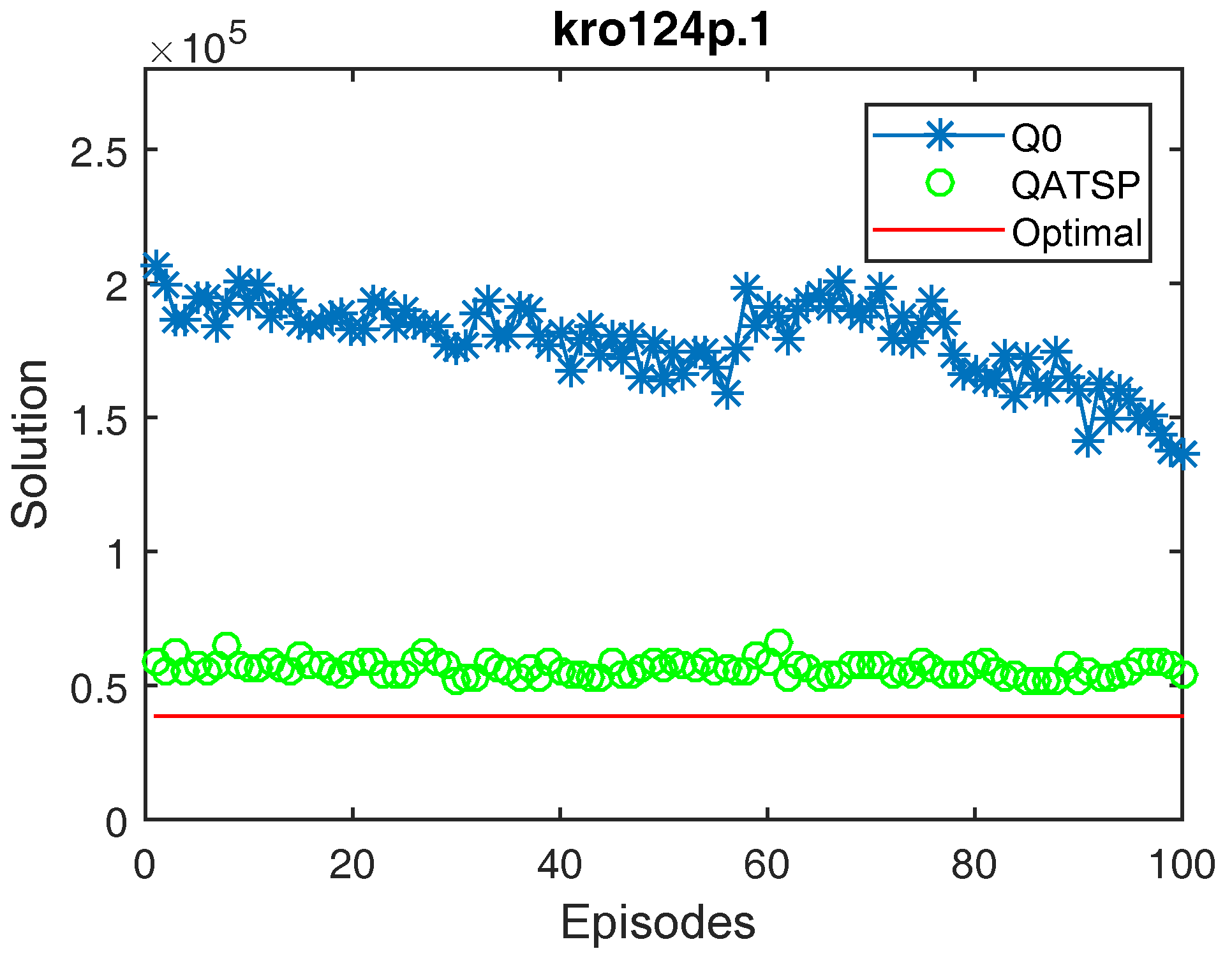
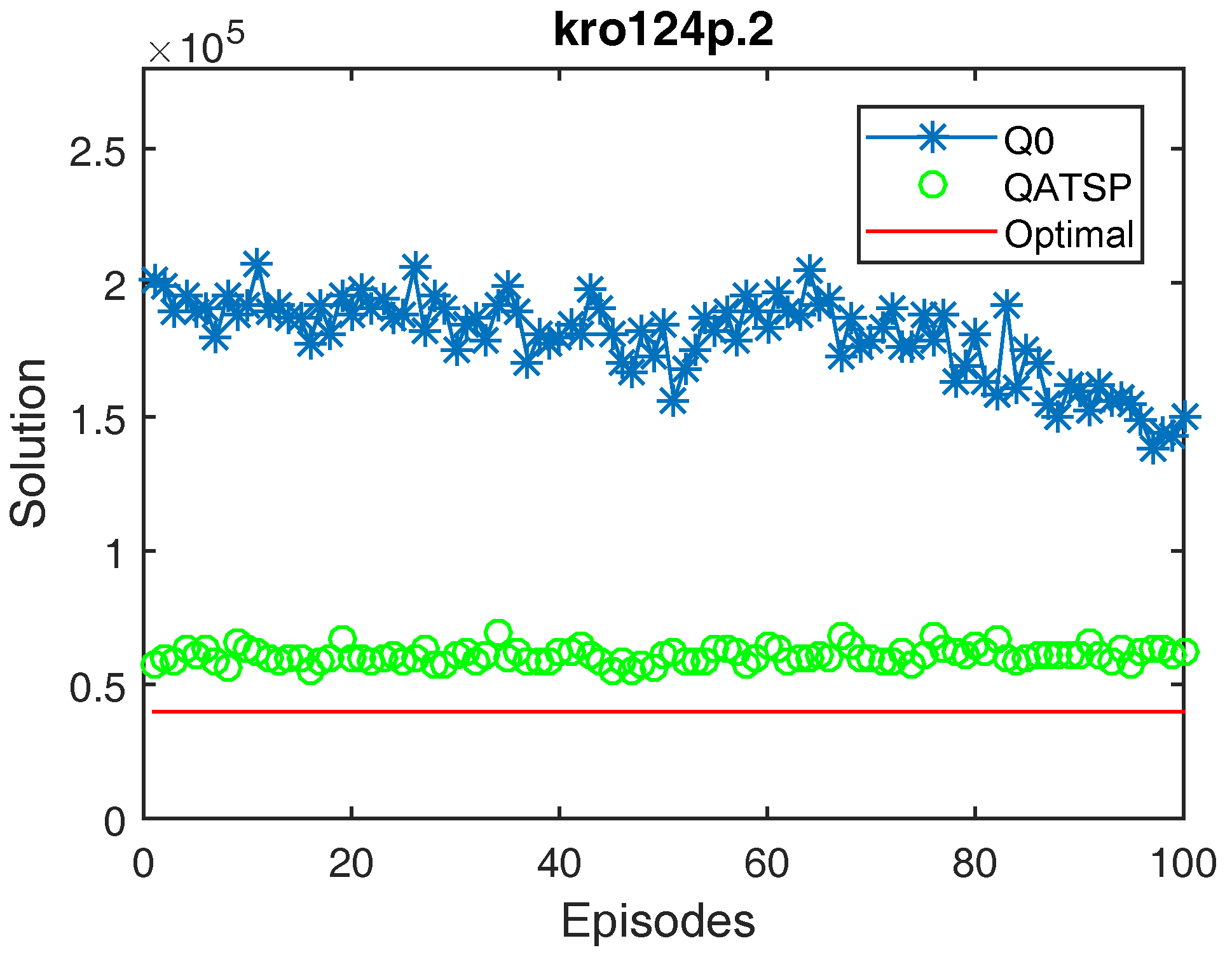
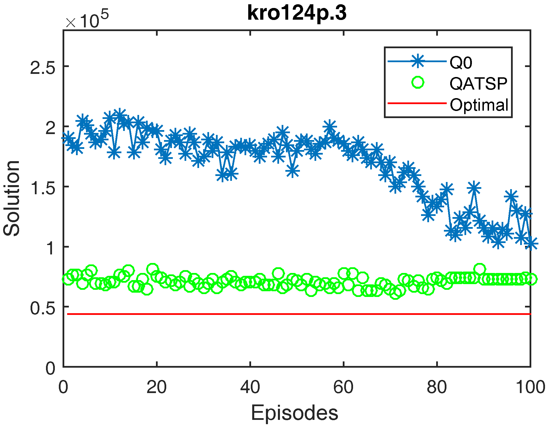
In this stage, the learning evolution graphs (distance calculated over the episodes) are analyzed for the following SOP problems: kro124p.1, kro124p.2, kro124p.3 and kro124p.4. These four problems are based on kro124p (ATSP), and the data between these instances vary depending on the number and arrangement of precedence constraints between the nodes (see Table 1 and Table 5).
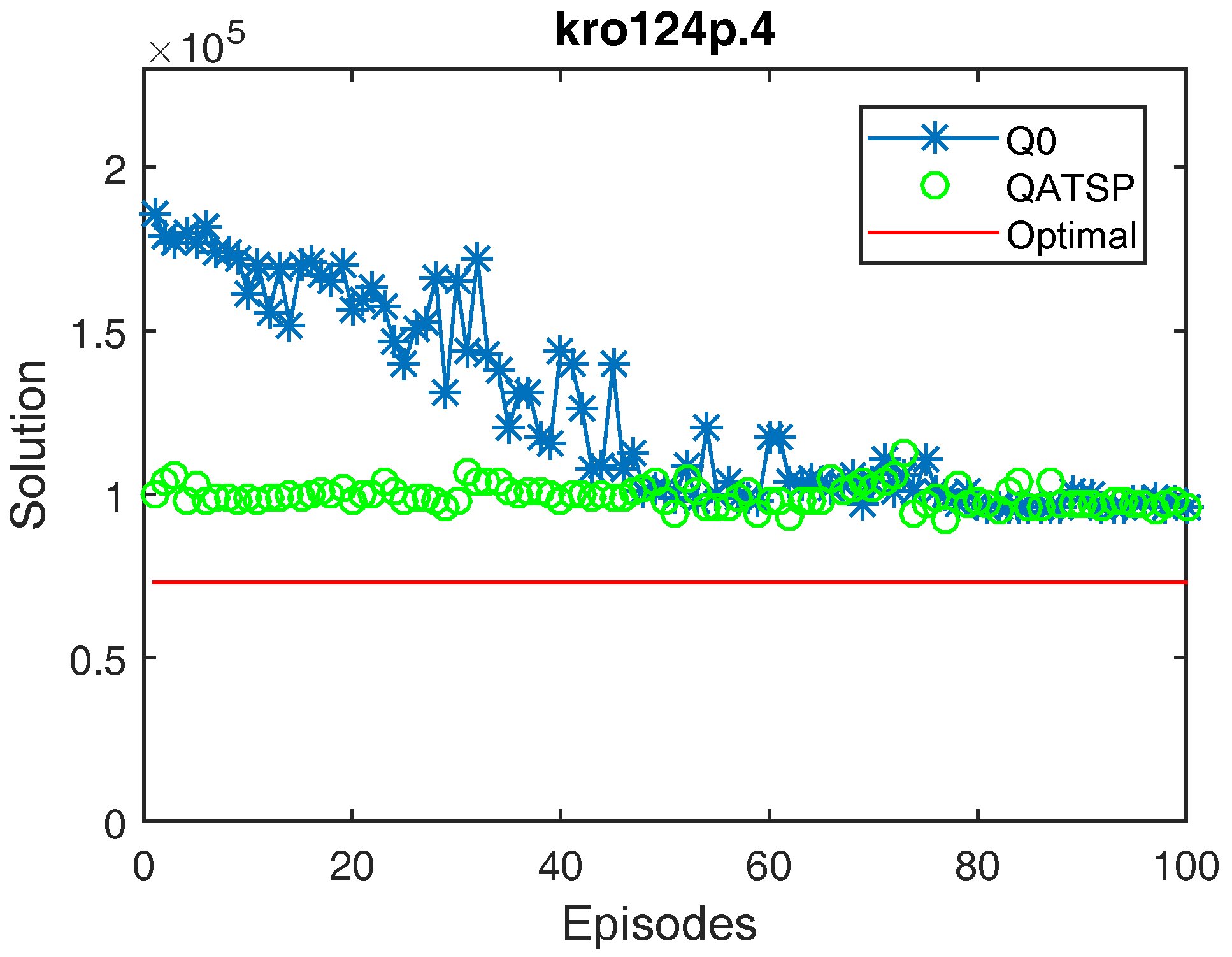
Figure 4, Figure 5, Figure 6 and Figure 7 show that the QATSP learning curves started the episodes closer to the optimal value of the instance than the simulations with Q0. This is most evident when comparing the values. In all the graphs shown, the difference between the solution in the initial episode of the QATSP and Q0 was greater than (80,000) distance units. This highlights the importance of transferring knowledge between the ATSP and SOP domains in the initial episodes, favoring the acceleration of learning.
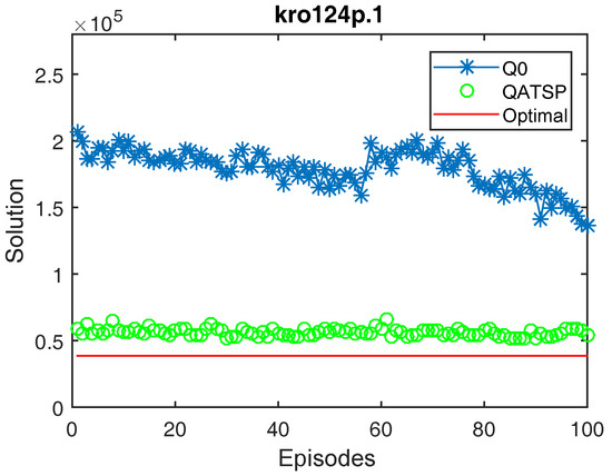
Figure 4.
Learning curves for the kro124p.1 instance (without learning transfer (QO) and with learning transfer (QATSP)) and TSPLIB’s optimal value line (38,762). Performance measures for Q0 ( = 206,824, = 136,261 and = 136,261) and QATSP ( = 58,497, = 54,649 and = 52,029).
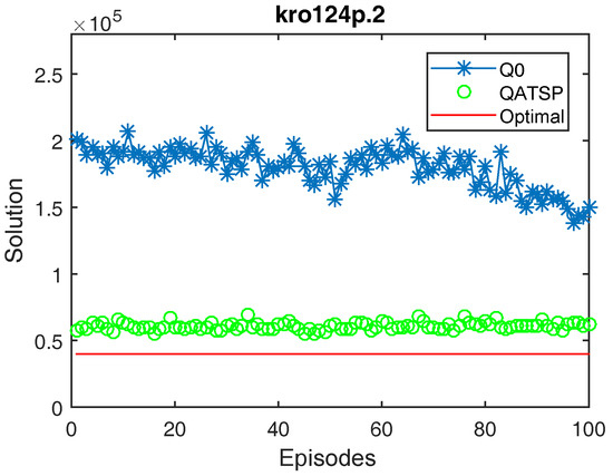
Figure 5.
Learning curves for the kro124p.2 instance (without learning transfer (QO) and with learning transfer (QATSP)) and TSPLIB’s optimal value line (39,841). Performance measures for Q0 ( = 201,214, = 150,206 and = 138,704) and QATSP ( = 57,230, = 62,778 and = 55,334).
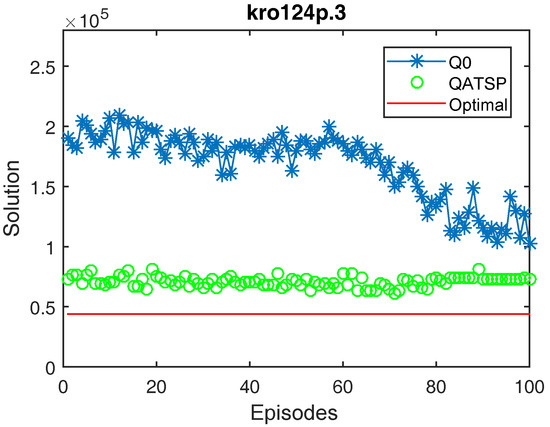
Figure 6.
Learning curves for the kro124p.3 instance (without learning transfer (QO) and with learning transfer (QATSP)) and TSPLIB’s optimal value line (43,904). Performance measures for Q0 ( = 190,308, = 102,856 and = 102,856) and QATSP ( = 73,178, = 73,407 and = 61,146).
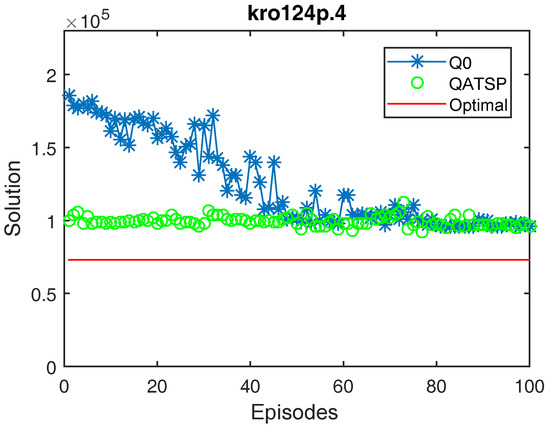
Figure 7.
Learning curves for the kro124p.4 instance (without learning transfer (QO) and with learning transfer (QATSP)) and TSPLIB’s optimal value line (73,021). Performance measures for Q0 ( = 186,028, = 96,283 and = 96,139) and QATSP ( = 99,903, = 95,602 and = 92,542).
In addition, the graphs in Figure 4, Figure 5 and Figure 6 also show the differences between the values for Q0 and the QATSP. For instances kro124p.1, kro124p.2 and kro124p.3, adopting transfer learning resulted in better results in the last episode of the simulation. In the worst case (experiments on problem kro124p.4), the Q0 learning curve still needed around 50 episodes to achieve results close to those presented by the simulations using the ATSP knowledge base.
Finally, it is worth highlighting that for the graphs presented in Figure 4, Figure 5, Figure 6 and Figure 7, employing transfer learning between the ATSP and SOP domains resulted in calculating better solutions during learning. For example, for the kro124p.1 instance, = 52,029 when adopting the QATSP, while for learning without prior knowledge, the result was = 136,261.
4.2. Results of Automated Transfer Learning
First, for comparison purposes, the selected SOP instances were run without using transfer learning. Next, the knowledge bases were generated using the ATSP instances at the time of execution of problems br17.10, p43.1, ry48p.1, ft53.1 and ft70.1. Thus, at the time of execution of these instances, all the stages of the proposed algorithm were executed.
For the remaining instances, as there was already a pre-existing knowledge base, only the first and third stages of the algorithm were run. Table 10 shows all the results obtained during the execution of the experiments.
Table 10.
Results of running SOP instances without the Auto_TL_RL algorithm and with the Auto_TL_RL algorithm, with the asymmetric traveling salesman problem (ATSP); sequential ordering problem (SOP); best known solution value presented by TSPLIB; and the proposed algorithm (Auto_TL_RL).
Based on the results shown in Table 10, it can be seen that the final distance achieved by the proposed transfer learning system showed better results in several of the instances tested, more precisely in 14 of the 18 instances (i.e., in approximately of the simulated SOP problems). Among these results, the final distance values obtained in instances ft70.4, ft70.1, ft53.4 and ry48p.4 stand out. In these four instances, there was a difference of more than 500 units in the values obtained when learning with the Auto_TL_RL system and without the Auto_TL_RL system. Consequently, it can be seen that by using the proposed Auto_TL_RL system, it was possible to obtain final distance values closer to those presented as the best known solution by TSPLIB compared with the results obtained when the Auto_TL_RL system was not used.
5. Comparison with Other Studies
This section presents a comparison of this proposal with other literature studies. For this, three papers that applied AI algorithms to solve the SOP were selected [37,39,80]. Table 11 shows a summary of this analysis.
Table 11.
Comparison of this proposal with different studies that applied algorithms for the sequential ordering problem’s solution.
The first point to emphasize is the relevance of the dataset used in this paper. In this sense, TSPLIB is frequently adopted in the literature when applying methods to combinatorial optimization problems, especially those related to the TSP and SOP.
The second criterion to be observed in Table 11 is the algorithm adopted to resolve SOP instances. Several traditional optimization techniques have already been used, such as the ant colony system [39] and particle swarm optimization [80]. It is noteworthy that the authors of [39,80] achieved important results in solving several TSPLIB instances, finding the best known solution in several simulated situations, thus showing great potential in these methods for solving combinatorial optimization problems based on the ATSP and SOP.
However, this paper did not aim to make a direct comparison with these conventional methods from the literature. The objective was to investigate and propose advances in reinforcement learning algorithms for solving combinatorial optimization problems. In this sense, it is noteworthy that, due to the best knowledge of these authors, this work is only the second paper that addresses reinforcement learning methods for solving the SOP.
For this aspect, the work in [37] made important advances in the application of RL and hyperparameter tuning for the SOP. For example, the work in [37] assessed that, in general, the SARSA algorithm outperforms the Q-learning method in the search for better SOP solutions. Following this line, this paper continued to investigate the possibilities for improving RL techniques for combinatorial optimization problems. The main advance of this paper in relation to the literature is the proposal of a transfer learning approach between the ATSP and SOP, providing a reduction in computational cost and optimization of the solution with RL algorithms. Furthermore, this paper innovated by proposing a new AutoML method, which is responsible for applying meta-learning and automatic TL between simulated combinatorial optimization problems.
6. Conclusions
The main objective of this work was to propose and evaluate the efficiency of a methodology for transfer RL between two combinatorial optimization domains: the ATSP and SOP. For this purpose, two approaches were taken. The first approach involved a general analysis of the transfer of learning. The second addressed the use of AutoML for transfer learning.
Based on the analysis performed, this work highlights certain aspects:
- Results visualization and interpretation of the impact on the final route distance results obtained with the transfer of learning between classical combinatorial optimization problems;
- Statistical analysis of the impact on the computational time and route distance results obtained by applying learning transfer between combinatorial optimization problems;
- Development of a methodology for learning transfer from the source domain (ATSP) to the target domain (SOP);
- Proposal of a methodology to perform learning transfer in an automated way;
- Proposal of an AutoML algorithm for transfer learning applied to combinatorial optimization problems with reinforcement learning.
In terms of analysis, the effects of using the knowledge base (QATSP) in the objective domain (SOP) were evaluated. The results obtained from the statistical tests show that, overall, adopting transfer learning led to the calculation of shorter routes in the SOP problems (TSPLIB). Furthermore, in 13 of the 14 instances simulated (), the average computational time was lower in the experiments using the QATSP base. Results visualization made it possible to evaluate the differences in the behavior of the learning curves when the RL transfer matrix was used or not used.
The AutoML approach involved the development of the Auto_TL_RL algorithm. The Auto_TL_RL algorithm has a feature that makes it possible to identify the presence or absence of a knowledge base for a given problem. When the knowledge base already exists, the issue is executed directly. However, when a previous knowledge base is not available, a knowledge base is generated and stored for possible reuse in future situations. To accomplish this, concepts discussed in [79] were used, such as transfer learning and automated learning.
The transfer learning performed by the Auto_TL_RL algorithm produced better results in 14 of the 18 TSPLIB instances analyzed (approximately ). This demonstrates its efficiency and importance compared with traditional learning methods. It is also important to highlight the importance of automated transfer, since all the human and computational effort required to carry out this study was reduced by using an automated learning system.
In future work, it is expected to apply the proposed approach to other combinatorial optimization problems. For this aspect, it is important to observe the three criteria presented when carrying out transfer reinforcement learning across combinatorial optimization problems: (1) problems with the same objective function; (2) similar datasets; and (3) transfer from the simple domain to the more complex domain. Moreover, a forthcoming paper will analyze the transfer of hyperparameter tuning between the domains: , , and the reinforcement function [12,37,68,76]. Moreover, the aim is to conduct the experiment with different instances. It is also intended to improve the Auto_TL_RL system in order to make it possible to apply the parameters used during the knowledge base generation stage, which showed the best results. Furthermore, future work will analyze the energy efficiency of the AUTO_TL_RL algorithm and its CO2 emissions, since the computational time can hide particularities in energy consumption.
Author Contributions
Methodology, G.K.B.S. and A.L.C.O.; software, G.K.B.S. and A.L.C.O.; validation, M.S.O. and D.C.R.O.; formal analysis, M.S.O. and D.C.R.O.; writing—original draft, G.K.B.S. and S.O.S.S.; writing—review and editing, S.O.S.S., A.L.C.O. and E.G.N.; supervision, E.G.N. All authors have read and agreed to the published version of the manuscript.
Funding
This publication has emanated from research supported in part by a grant from Science Foundation Ireland under Grant number 18/CRT/6049 (Author: Samara O. S. Santos). For the purpose of Open Access, the author (Samara O. S. Santos) has applied a CC BY public copyright licence to any Author Accepted Manuscript version arising from this submission. Erivelton G. Nepomuceno was supported by Brazilian Research Agencies: CNPq/INERGE (Grant No. 465704/2014-0), CNPq (Grant No. 425509/2018-4) and FAPEMIG (Grant No. APQ-00870-17). This publication has emanated from research conducted with the financial support of Science Foundation Ireland under Grant number 21/FFP-P/10065.
Data Availability Statement
The dataset analyzed during the current study is available from the TSPLIB repository (http://comopt.ifi.uni-heidelberg.de/software/TSPLIB95/, accessed on 1 December 2023).
Acknowledgments
The authors are grateful to UFRB, Maynooth University, UFSJ, FAPEMIG, CNPq/INERGE and Science Foundation Ireland.
Conflicts of Interest
The authors declare no conflicts of interest.
Abbreviations
The following abbreviations are used in this manuscript:
| Reinforcement learning | |
| Machine learning | |
| Automated machine learning | |
| Automated reinforcement learning | |
| Transfer learning | |
| Traveling salesman problem | |
| Asymmetric traveling salesman problem | |
| Sequential ordering problem | |
| Traveling Salesman Problem Library | |
| automated transfer reinforcement learning algorithm | |
| Markov decision processes | |
| S | State |
| s | Current state |
| New state | |
| A | Action |
| a | Current action |
| New action | |
| R | Reinforcements |
| T | State transition model |
| t | Statistical test |
| Q | Learning matrix |
| Learning matrix at the current time | |
| Learning matrix at a future time | |
| Distance calculated in the initial episode | |
| Distance in the final episode | |
| Smallest solution found | |
| Matrix started with null values | |
| Matrix from ATSP instance | |
| Cost between cities i and j | |
| State–action–reward–state–action | |
| N | Number of nodes |
| Kolmogorov–Smirnov |
References
- Ghanem, M.C.; Chen, T.M.; Nepomuceno, E.G. Hierarchical reinforcement learning for efficient and effective automated penetration testing of large networks. J. Intell. Inf. Syst. 2023, 60, 281–303. [Google Scholar] [CrossRef]
- Watkins, C.J.; Dayan, P. Technical note Q-learning. Mach. Learn. 1992, 8, 279–292. [Google Scholar] [CrossRef]
- Russell, S.J.; Norving, P. Artificial Intelligence, 3rd ed.; Pearson: Upper Saddle River, NJ, USA, 2013. [Google Scholar]
- Sutton, R.; Barto, A. Reinforcement Learning: An Introduction, 2nd ed.; MIT Press: Cambridge, MA, USA, 2018. [Google Scholar]
- Vazquez-Canteli, J.R.; Nagy, Z. Reinforcement learning for demand response: A review of algorithms and modeling techniques. Appl. Energy 2019, 235, 1072–1089. [Google Scholar] [CrossRef]
- Mazyavkina, N.; Sviridov, S.; Ivanov, S.; Burnaev, E. Reinforcement learning for combinatorial optimization: A survey. Comput. Oper. Res. 2021, 134, 105400. [Google Scholar] [CrossRef]
- Ruiz-Serra, J.; Harré, M.S. Inverse Reinforcement Learning as the Algorithmic Basis for Theory of Mind: Current Methods and Open Problems. Algorithms 2023, 16, 68. [Google Scholar] [CrossRef]
- Deák, S.; Levine, P.; Pearlman, J.; Yang, B. Reinforcement Learning in a New Keynesian Model. Algorithms 2023, 16, 280. [Google Scholar] [CrossRef]
- Engelhardt, R.C.; Oedingen, M.; Lange, M.; Wiskott, L.; Konen, W. Iterative Oblique Decision Trees Deliver Explainable RL Models. Algorithms 2023, 16, 282. [Google Scholar] [CrossRef]
- Parker-Holder, J.; Rajan, R.; Song, X.; Biedenkapp, A.; Miao, Y.; Eimer, T.; Zhang, B.; Nguyen, V.; Calandra, R.; Faust, A.; et al. Automated Reinforcement Learning (AutoRL): A Survey and Open Problems. J. Artif. Intell. Res. 2022, 74, 517–568. [Google Scholar] [CrossRef]
- Afshar, R.R.; Zhang, Y.; Vanschoren, J.; Kaymak, U. Automated Reinforcement Learning: An Overview. arXiv 2022, arXiv:2201.05000. [Google Scholar]
- Brazdil, P.; van Rijn, J.N.; Soares, C.; Vanschoren, J. Metalearning: Applications to Automated Machine Learning and Data Mining; Springer Nature: Berlin/Heidelberg, Germany, 2022. [Google Scholar]
- Feurer, M.; Klein, A.; Eggensperger, K.; Springenberg, J.; Blum, M.; Hutter, F. Efficient and Robust Automated Machine Learning. In Advances in Neural Information Processing Systems; Cortes, C., Lawrence, N., Lee, D., Sugiyama, M., Garnett, R., Eds.; Curran Associates, Inc.: Red Hook, NY, USA, 2015; Volume 28, pp. 2962–2970. [Google Scholar]
- Tuggener, L.; Amirian, M.; Rombach, K.; Lorwald, S.; Varlet, A.; Westermann, C.; Stadelmann, T. Automated Machine Learning in Practice: State of the Art and Recent Results. In Proceedings of the 2019 6th Swiss Conference on Data Science (SDS), Bern, Switzerland, 14 June 2019; pp. 31–36. [Google Scholar] [CrossRef]
- Chen, L.; Hu, B.; Guan, Z.H.; Zhao, L.; Shen, X. Multiagent Meta-Reinforcement Learning for Adaptive Multipath Routing Optimization. IEEE Trans. Neural Netw. Learn. Syst. 2022, 33, 5374–5386. [Google Scholar] [CrossRef] [PubMed]
- Dai, H.; Chen, P.; Yang, H. Metalearning-Based Fault-Tolerant Control for Skid Steering Vehicles under Actuator Fault Conditions. Sensors 2022, 22, 845. [Google Scholar] [CrossRef]
- Taylor, M.E.; Stone, P. Transfer Learning for Reinforcement Learning Domains: A Survey. J. Mach. Learn. Res. 2009, 10, 1633–1685. [Google Scholar]
- Carroll, J.L.; Peterson, T. Fixed vs. Dynamic Sub-Transfer in Reinforcement Learning. In Proceedings of the International Conference on Machine Learning and Applications, Las Vegas, NV, USA, 24–27 June 2002; pp. 3–8. [Google Scholar]
- Cao, Z.; Kwon, M.; Sadigh, D. Transfer Reinforcement Learning Across Homotopy Classes. IEEE Robot. Autom. Lett. 2021, 6, 2706–2713. [Google Scholar] [CrossRef]
- Peterson, T.S.; Owens, N.E.; Carroll, J.L. Towards automatic shaping in robot navigation. In Proceedings of the 2001 ICRA. IEEE International Conference on Robotics and Automation (Cat. No.01CH37164), Seoul, Republic of Korea, 21–26 May 2001; Volume 1, pp. 517–522. [Google Scholar]
- Wang, H.; Fan, S.; Song, J.; Gao, Y.; Chen, X. Reinforcement learning transfer based on subgoal discovery and subtask similarity. IEEE/CAA J. Autom. Sin. 2014, 1, 257–266. [Google Scholar]
- Tommasino, P.; Caligiore, D.; Mirolli, M.; Baldassarre, G. A Reinforcement Learning Architecture That Transfers Knowledge Between Skills When Solving Multiple Tasks. IEEE Trans. Cogn. Dev. Syst. 2019, 11, 292–317. [Google Scholar]
- Arnekvist, I.; Kragic, D.; Stork, J.A. VPE: Variational Policy Embedding for Transfer Reinforcement Learning. In Proceedings of the 2019 International Conference on Robotics and Automation (ICRA), Montreal, QC, Canada, 20–24 May 2019; pp. 36–42. [Google Scholar]
- Gao, D.; Wang, S.; Yang, Y.; Zhang, H.; Chen, H.; Mei, X.; Chen, S.; Qiu, J. An Intelligent Control Method for Servo Motor Based on Reinforcement Learning. Algorithms 2024, 17, 14. [Google Scholar] [CrossRef]
- Hou, Y.; Ong, Y.S.; Feng, L.; Zurada, J.M. An Evolutionary Transfer Reinforcement Learning Framework for Multiagent Systems. IEEE Trans. Evol. Comput. 2017, 21, 601–615. [Google Scholar] [CrossRef]
- Da Silva, F.; Reali Costa, A. A survey on transfer learning for multiagent reinforcement learning systems. J. Artif. Intell. Res. 2019, 64, 645–703. [Google Scholar] [CrossRef]
- Cai, L.; Sun, Q.; Xu, T.; Ma, Y.; Chen, Z. Multi-AUV Collaborative Target Recognition Based on Transfer-Reinforcement Learning. IEEE Access 2020, 8, 39273–39284. [Google Scholar] [CrossRef]
- Ottoni, A.L.; Nepomuceno, E.G.; Oliveira, M.S.d.; Oliveira, D.C.d. Reinforcement learning for the traveling salesman problem with refueling. Complex Intell. Syst. 2022, 8, 2001–2015. [Google Scholar] [CrossRef]
- Gambardella, L.M.; Dorigo, M. Ant-Q: A reinforcement learning approach to the traveling salesman problem. In Proceedings of the 12th International Conference on Machine Learning, Tahoe, CA, USA, 9–12 July 1995; pp. 252–260. [Google Scholar]
- Bianchi, R.A.C.; Ribeiro, C.H.C.; Costa, A.H.R. On the relation between Ant Colony Optimization and Heuristically Accelerated Reinforcement Learning. In Proceedings of the 1st International Workshop on Hybrid Control of Autonomous System, Pasadena, CA, USA, 13 July 2009; pp. 49–55. [Google Scholar]
- Júnior, F.C.D.L.; Neto, A.D.D.; De Melo, J.D. Hybrid metaheuristics using reinforcement learning applied to salesman traveling problem. In Traveling Salesman Problem, Theory and Applications; IntechOpen: London, UK, 2010. [Google Scholar]
- Costa, M.L.; Padilha, C.A.A.; Melo, J.D.; Neto, A.D.D. Hierarchical Reinforcement Learning and Parallel Computing Applied to the k-server Problem. IEEE Lat. Am. Trans. 2016, 14, 4351–4357. [Google Scholar] [CrossRef]
- Alipour, M.M.; Razavi, S.N.; Feizi Derakhshi, M.R.; Balafar, M.A. A Hybrid Algorithm Using a Genetic Algorithm and Multiagent Reinforcement Learning Heuristic to Solve the Traveling Salesman Problem. Neural Comput. Appl. 2018, 30, 2935–2951. [Google Scholar] [CrossRef]
- Lins, R.A.S.; Dória, A.D.N.; de Melo, J.D. Deep reinforcement learning applied to the k-server problem. Expert Syst. Appl. 2019, 135, 212–218. [Google Scholar] [CrossRef]
- Carvalho Ottoni, A.L.; Geraldo Nepomuceno, E.; Santos de Oliveira, M. Development of a Pedagogical Graphical Interface for the Reinforcement Learning. IEEE Lat. Am. Trans. 2020, 18, 92–101. [Google Scholar] [CrossRef]
- Silva, M.A.L.; de Souza, S.R.; Souza, M.J.F.; Bazzan, A.L.C. A reinforcement learning-based multi-agent framework applied for solving routing and scheduling problems. Expert Syst. Appl. 2019, 131, 148–171. [Google Scholar] [CrossRef]
- Ottoni, A.L.C.; Nepomuceno, E.G.; de Oliveira, M.S.; de Oliveira, D.C.R. Tuning of Reinforcement Learning Parameters Applied to SOP Using the Scott–Knott Method. Soft Comput. 2020, 24, 4441–4453. [Google Scholar] [CrossRef]
- Escudero, L. An inexact algorithm for the sequential ordering problem. Eur. J. Oper. Res. 1988, 37, 236–249. [Google Scholar] [CrossRef]
- Gambardella, L.M.; Dorigo, M. An Ant Colony System Hybridized with a New Local Search for the Sequential Ordering Problem. Informs J. Comput. 2000, 12, 237–255. [Google Scholar] [CrossRef]
- Letchford, A.N.; Salazar-González, J.J. Stronger multi-commodity flow formulations of the (capacitated) sequential ordering problem. Eur. J. Oper. Res. 2016, 251, 74–84. [Google Scholar] [CrossRef]
- Skinderowicz, R. An improved Ant Colony System for the Sequential Ordering Problem. Comput. Oper. Res. 2017, 86, 1–17. [Google Scholar] [CrossRef]
- Hopfield, J.; Tank, D. “Neural” computation of decisions in optimization problems. Biol. Cybern. 1985, 52, 141–152. [Google Scholar] [CrossRef]
- Jäger, G.; Molitor, P. Algorithms and experimental study for the traveling salesman problem of second order. In Proceedings of the Second International Conference, COCOA 2008, St. John’s, NL, Canada, 21–24 August 2008; Lecture Notes in Computer Science (including subseries Lecture Notes in Artificial Intelligence and Lecture Notes in Bioinformatics); 5165 LNCS. pp. 211–224. [Google Scholar] [CrossRef]
- Takashima, Y.; Nakamura, Y. Theoretical and Experimental Analysis of Traveling Salesman Walk Problem. In Proceedings of the 2021 IEEE Asia Pacific Conference on Circuit and Systems (APCCAS), Penang, Malaysia, 22–26 November 2021; pp. 241–244. [Google Scholar]
- Alhenawi, E.; Khurma, R.A.; Damaševičius, R.; Hussien, A.G. Solving Traveling Salesman Problem Using Parallel River Formation Dynamics Optimization Algorithm on Multi-core Architecture Using Apache Spark. Int. J. Comput. Intell. Syst. 2024, 17, 4. [Google Scholar] [CrossRef]
- Shobaki, G.; Jamal, J. An exact algorithm for the sequential ordering problem and its application to switching energy minimization in compilers. Comput. Optim. Appl. 2015, 61, 343–372. [Google Scholar] [CrossRef]
- Libralesso, L.; Bouhassoun, A.; Cambazard, H.; Jost, V. Tree search algorithms for the Sequential Ordering Problem. arXiv 2019, arXiv:abs/1911.12427. [Google Scholar]
- Tavares Neto, R.F.; Godinho Filho, M.; Da Silva, F.M. An ant colony optimization approach for the parallel machine scheduling problem with outsourcing allowed. J. Intell. Manuf. 2015, 26, 527–538. [Google Scholar] [CrossRef]
- Reinelt, G. TSPLIB—A Traveling Salesman Problem Library. ORSA J. Comput. 1991, 3, 376–384. [Google Scholar] [CrossRef]
- Reinelt, G. Tsplib95; University Heidelberg: Heidelberg, Germany, 1995. [Google Scholar]
- Liu, Y.; Cao, B.; Li, H. Improving ant colony optimization algorithm with epsilon greedy and Levy flight. Complex Intell. Syst. 2021, 7, 1711–1722. [Google Scholar] [CrossRef]
- Goldbarg, M.C.; Luna, H. Combinatorial Optimization and Linear Programming: Models and Algorithms; Elsevier Publishing House: Rio de Janeiro, Brazil, 2015. [Google Scholar]
- Queiroz dos Santos, J.P.; de Melo, J.D.; Duarte Neto, A.D.; Aloise, D. Reactive Search strategies using Reinforcement Learning, local search algorithms and Variable Neighborhood Search. Expert Syst. Appl. 2014, 41, 4939–4949. [Google Scholar] [CrossRef]
- Almeida, C.P.d.; Gonçalves, R.A.; Goldbarg, E.F.; Goldbarg, M.C.; Delgado, M.R. Transgenetic Algorithms for the Multi-objective Quadratic Assignment Problem. In Proceedings of the 2014 Brazilian Conference on Intelligent Systems, Sao Paulo, Brazil, 18–22 October 2014; pp. 312–317. [Google Scholar] [CrossRef]
- Bengio, Y.; Lodi, A.; Prouvost, A. Machine Learning for Combinatorial Optimization: A Methodological Tour d’Horizon. arXiv 2018, arXiv:1811.06128. [Google Scholar] [CrossRef]
- Bianchi, R.A.; Celiberto, L.A., Jr.; Santos, P.E.; Matsuura, J.P.; De Mantaras, R.L. Transferring knowledge as heuristics in reinforcement learning: A case-based approach. Artif. Intell. 2015, 226, 102–121. [Google Scholar] [CrossRef]
- Pedro, O.; Saldanha, R.; Camargo, R. A tabu search approach for the prize collecting traveling salesman problem. Electron. Notes Discret. Math. 2013, 41, 261–268. [Google Scholar] [CrossRef]
- Montemanni, R.; Dell’Amico, M. Solving the Parallel Drone Scheduling Traveling Salesman Problem via Constraint Programming. Algorithms 2023, 16, 40. [Google Scholar] [CrossRef]
- Bodin, L.; Golden, B.; Assad, A.; Ball, M. Routing and Scheduling of Vehicles and Crews—The State of the Art. Comput. Oper. Res. 1983, 10, 63–211. [Google Scholar]
- Majidi, F.; Openja, M.; Khomh, F.; Li, H. An Empirical Study on the Usage of Automated Machine Learning Tools. In Proceedings of the 2022 IEEE International Conference on Software Maintenance and Evolution (ICSME), Limassol, Cyprus, 2–7 October 2022; pp. 59–70. [Google Scholar]
- Ottoni, A.L.C.; Souza, A.M.; Novo, M.S. Automated hyperparameter tuning for crack image classification with deep learning. Soft Comput. 2023, 27, 18383–18402. [Google Scholar] [CrossRef]
- Barreto, C.A.d.S.; Canuto, A.M.d.P.; Xavier-Júnior, J.C.; Feitosa-Neto, A.; Lima, D.F.A.; Costa, R.R.F.d. PBIL AutoEns: An Automated Machine Learning Tool integrated to the Weka ML Platform. Braz. J. Dev. 2019, 5, 29226–29242. [Google Scholar] [CrossRef]
- Chauhan, K.; Jani, S.; Thakkar, D.; Dave, R.; Bhatia, J.; Tanwar, S.; Obaidat, M.S. Automated Machine Learning: The New Wave of Machine Learning. In Proceedings of the 2020 2nd International Conference on Innovative Mechanisms for Industry Applications (ICIMIA), Bangalore, India, 5–7 March 2020; pp. 205–212. [Google Scholar] [CrossRef]
- Olson, R.S.; Moore, J.H. TPOT: A tree-based pipeline optimization tool for automating machine learning. In Proceedings of the Workshop on Automatic Machine Learning, New York, NY, USA, 24 June 2016; pp. 66–74. [Google Scholar]
- Li, Y.; Wu, J.; Deng, T. Meta-GNAS: Meta-reinforcement learning for graph neural architecture search. Eng. Appl. Artif. Intell. 2023, 123, 106300. [Google Scholar] [CrossRef]
- Ottoni, L.T.C.; Ottoni, A.L.C.; Cerqueira, J.d.J.F. A Deep Learning Approach for Speech Emotion Recognition Optimization Using Meta-Learning. Electronics 2023, 12, 4859. [Google Scholar] [CrossRef]
- Mantovani, R.G.; Rossi, A.L.D.; Alcobaça, E.; Vanschoren, J.; de Carvalho, A.C.P.L.F. A meta-learning recommender system for hyperparameter tuning: Predicting when tuning improves SVM classifiers. Inf. Sci. 2019, 501, 193–221. [Google Scholar] [CrossRef]
- Hutter, F.; Kotthoff, L.; Vanschoren, J. (Eds.) Automated Machine Learning: Methods, Systems, Challenges; Springer: Berlin/Heidelberg, Germany, 2019; in press; Available online: http://automl.org/book (accessed on 1 December 2023).
- Fernández, F.; Veloso, M. Probabilistic policy reuse in a reinforcement learning agent. In Proceedings of the Fifth International Joint Conference on Autonomous Agents and Multiagent Systems, Hakodate, Japan, 8–12 May 2006; pp. 720–727. [Google Scholar]
- Feng, Y.; Wang, G.; Liu, Z.; Feng, R.; Chen, X.; Tai, N. An Unknown Radar Emitter Identification Method Based on Semi-Supervised and Transfer Learning. Algorithms 2019, 12, 271. [Google Scholar] [CrossRef]
- Pavlyuk, D. Transfer Learning: Video Prediction and Spatiotemporal Urban Traffic Forecasting. Algorithms 2020, 13, 39. [Google Scholar] [CrossRef]
- Islam, M.M.; Hossain, M.B.; Akhtar, M.N.; Moni, M.A.; Hasan, K.F. CNN Based on Transfer Learning Models Using Data Augmentation and Transformation for Detection of Concrete Crack. Algorithms 2022, 15, 287. [Google Scholar] [CrossRef]
- Surendran, R.; Chihi, I.; Anitha, J.; Hemanth, D.J. Indoor Scene Recognition: An Attention-Based Approach Using Feature Selection-Based Transfer Learning and Deep Liquid State Machine. Algorithms 2023, 16, 430. [Google Scholar] [CrossRef]
- Pavliuk, O.; Mishchuk, M.; Strauss, C. Transfer Learning Approach for Human Activity Recognition Based on Continuous Wavelet Transform. Algorithms 2023, 16, 77. [Google Scholar] [CrossRef]
- Durgut, R.; Aydin, M.E.; Rakib, A. Transfer Learning for Operator Selection: A Reinforcement Learning Approach. Algorithms 2022, 15, 24. [Google Scholar] [CrossRef]
- Ottoni, A.L.C.; Nepomuceno, E.G.; de Oliveira, M.S. A Response Surface Model Approach to Parameter Estimation of Reinforcement Learning for the Travelling Salesman Problem. J. Control. Autom. Electr. Syst. 2018, 29, 350–359. [Google Scholar] [CrossRef]
- Montgomery, D.C. Design and Analysis of Experiments, 9th ed.; John Wiley & Sons.: New York, NY, USA, 2017. [Google Scholar]
- Lopes, R.H. Kolmogorov-Smirnov Test. Int. Encycl. Stat. Sci. 2011, 1, 718–720. [Google Scholar]
- Souza, G.K.B.; Ottoni, A.L.C. AutoRL-TSP-RSM: Automated reinforcement learning system with response surface methodology for the traveling salesman problem. Braz. J. Appl. Comput. 2021, 13, 86–100. [Google Scholar] [CrossRef]
- Anghinolfi, D.; Montemanni, R.; Paolucci, M.; Gambardella, L.M. A hybrid particle swarm optimization approach for the sequential ordering problem. Comput. Oper. Res. 2011, 38, 1076–1085. [Google Scholar] [CrossRef]

Disclaimer/Publisher’s Note: The statements, opinions and data contained in all publications are solely those of the individual author(s) and contributor(s) and not of MDPI and/or the editor(s). MDPI and/or the editor(s) disclaim responsibility for any injury to people or property resulting from any ideas, methods, instructions or products referred to in the content. |
© 2024 by the authors. Licensee MDPI, Basel, Switzerland. This article is an open access article distributed under the terms and conditions of the Creative Commons Attribution (CC BY) license (https://creativecommons.org/licenses/by/4.0/).