A Novel Higher-Order Numerical Scheme for System of Nonlinear Load Flow Equations

Abstract

Power flow problems can be solved in a variety of ways by using the Newton–Raphson approach. The nonlinear power flow equations depend upon voltages $\left|V_i\right|$ and phase angle $\delta$. An electrical power system is obtained by taking the partial derivatives of load flow equations which contain active and reactive powers. In this paper, we present an efficient seventh-order iterative scheme to obtain the solutions of nonlinear system of equations, with only three steps in its formulation. Then, we illustrate the computational cost for different operations such as matrix–matrix multiplication, matrix–vector multiplication, and LU-decomposition, which is then used to calculate the cost of our proposed method and is compared with the cost of already seventh-order methods. Furthermore, we elucidate the applicability of our newly developed scheme in an electrical power system. The two-bus, three-bus, and four-bus power flow problems are then solved by using load flow equations that describe the applicability of the new schemes.

1. Introduction

In numerical analysis, we investigate, develop, and analyze numerous methods and algorithms for numerically solving real-life problems in the diverse domains of science such as physics, chemistry, mechanical engineering, chemical engineering, electrical engineering, and other applied sciences. Various kinds of efficient iterative methods are constructed to approximate the roots of system of nonlinear equations of the form

$$F\left(X\right)=0,$$

(1)

where $F:\mathbb{D}\subseteq {\mathbb{R}}^m\to {\mathbb{R}}^m$ with $m>1$ for multivariate function. One of the powerful and simplest root finding methods to solve the system of nonlinear equations is Newton–Raphson technique, expressed as

$$X^{(k+1)}=X^{\left(k\right)}-F^{\prime }{\left(X^{\left(k\right)}\right)}^{-1}F\left(X^{\left(k\right)}\right),$$

(2)

where $\left[F^{\prime }\left(X^{\left(k\right)}\right)\right]$ is the Jacobian matrix evaluated in the iterate $X^{\left(k\right)}$. This involves one function and one Jacobian evaluation at each step. Over the passage of time, the higher-order and computationally efficient variants are developed to solve the large-scale real-world problems.

Many researchers have introduced multipoint iterative schemes as a solution to the limitations of one-point iterative approaches. For example, in 1969, Jarratt [1] developed a fourth-order two-step optimal method. Some researchers have also developed fifth- and sixth-order techniques in an effort to obtain faster algorithms, as seen, for instance, in [2,3,4]. However, there are only a few Jarratt-type seventh-order iterative schemes for solving nonlinear systems [5,6] that have less computational cost. Another line of research is based on Steffensen’s method for solving nonlinear systems, following which some seventh-order derivative-free schemes were designed [7,8,9,10,11]. It is evident that while efforts are being made by the researchers to enhance the order of convergence of an iterative approach, most of the time, this results in an increase in the computational cost per iteration, for example, the seventh- and eighth-order methods developed recently [12,13,14,15,16]. Therefore, even when we create new iterative techniques, we ought to make an effort to minimize the computing expense.

Highly convergent multipoint iterative schemes can be categorized in two different ways: first, by developing a new scheme for scalar equations and then extending the same scheme for multidimensional cases with the same convergence order as that for the scalar equations; and second, developing the iterative schemes for system of equations with the help of different approaches like divided difference approach, quadratic formula, etc. Optimal Jarratt fourth-order two-step method and schemes by Abad et al. [5], Yaseen et al. [6], Behl et al. [2], and Lee and Kim [4] are extendable for a multidimensional case in a way that is described in the first category. On the other hand, Hueso et al. [3] proposed the fourth-order method for multivariate case and Sharma et al. [17] developed some fourth- and sixth-order schemes by using the weight function approach. It seems like the first technique is an easy way to develop some multidimensional iterative methods, but this is not the case. The key objective is to retain the order of convergence of the described scheme while extending it to the multidimensional case.

Nonlinear systems of equations are commonly used to describe scientific and engineering challenges. There are more and more applications for these systems, and the majority of the techniques, now in use, have limitations and drawbacks. Thus, it is crucial to create novel numerical techniques that are computationally efficient, fast and reliable. Among the problems of electrical engineering, load flow studies are important in planning and designing the future expansion of power systems [18,19,20,21]. Planning the expansion of power systems and figuring out how to operate the current systems most effectively require a load-flow study. Additionally, it serves as the foundation for a number of studies that demand quick processing times, such as those on online applications, optimal power flow, and continuation power flow. Energy passes from the generator to the load in a power system through numerous networks. The flow of active power P and reactive power Q is referred to as the load flow. In a steady-state analysis of a power system, power flow analysis is an effective approach, and many iterative strategies for solving power flow equations were developed by researchers; in 1956, the first automated digital solution to the power flow problem was given by Ward and Hale [22]. The study of power flow analysis gives different techniques for determining various bus components such as active power, reactive power, voltage magnitude $\left|V\right|$, and phase angle $\delta$ in a power grid. The resulting equations are known as power flow equations. A power flow study’s goal is to determine the voltages (magnitude and angle) for a specific load, generation, and network state. Line flows and losses can be computed after the voltages for each bus are known. Determining the known and unknown factors in the system is the first step towards solving power flow issues.

Table 1. Classification of buses.

Types of Bus	Specified Quantities	Unspecified Quantities
Slack bus	$\left|V\right|,\delta$	$P,Q$
Generator/$PV$ bus	$P,\left|V\right|$	$Q,\delta$
Load/$PQ$ bus	$P,Q$	$\left|V\right|,\delta$

illustrates the three categories of buses that are created based on these variables: reference/slack/swing bus, generator/$PV$ bus, and load/$PQ$ bus. Each bus specifies active and reactive power in a three-phase system. To solve the power flow equations, each bus consists of two defined and two unidentified variables.

To provide the mismatch between scheduled generation, total system load (including losses), and total generation, the slack bus is necessary. Each generator bus has a predetermined value of real power P excluding a slack bus. As a result of the specification of both voltage magnitude and angles, the slack bus, also known as the swing bus, is sometimes regarded as the reference bus. Because the net real power is specified and the voltage magnitude is regulated, the remaining generator buses are referred to as regulated or PV buses. Practical power systems have many load buses. Due to the specification of both net real and reactive power loads, load buses are also known as PQ buses. For PQ buses, both voltage magnitudes and angles are unknown, whereas for PV buses, only the voltage angle is unknown. For slack bus, voltage magnitude and angles are already known so there are no variables that are unknown. In a system with n buses and g generators, there are $2(n-1)-(g-1)$ unknowns. To solve these unknowns, real and reactive power balance equations are used. To obtain these equations, the transmission network is modeled using the admittance matrix (Y-bus). Under certain conditions, the magnitude of voltage V and phase angle at each bus in a power flow problems are calculated by using different iterative techniques.

Nodal power balancing equations must be solved in order to conduct power flow analysis. Due to the nonlinear nature of these equations, iterative approaches like the Newton–Raphson, Gauss–Seidel, fast-decoupled, modified Newton, DC load flow methods, and sparse matrix techniques are frequently employed to resolve this issue. The following are the advantages and disadvantages of these techniques:

• Gauss–Seidel Method:
  • Advantages: Simple implementation, low memory requirement, suitable for small to medium-sized systems.
  • Disadvantages: Slow convergence for large and highly nonlinear systems, may not converge for certain network configurations, sensitive to initial guesses.
• Newton–Raphson Method:
  • Advantages: Faster convergence compared to Gauss–Seidel, suitable for large and highly nonlinear systems, allows for simultaneous solution of multiple equations.
  • Disadvantages: Higher computational complexity, requires initial estimates for all variables, may encounter convergence issues for ill-conditioned systems. Moreover, it starts to lose its ability to converge fast with the increasing system size.
• Fast Decoupled Method:
  • Advantages: Improves convergence speed compared to Newton–Raphson, less computational burden, suitable for medium to large systems with moderate nonlinearity.
  • Disadvantages: Less accurate than Newton–Raphson, may not converge for highly nonlinear systems, requires assumptions to decouple real and reactive power calculations.
• Modified Newton Method:
  • Advantages: Combines advantages of Newton–Raphson and fast decoupled methods, faster convergence than traditional Newton–Raphson.
  • Disadvantages: May require more computational resources than fast decoupled method, convergence issues still possible for highly nonlinear systems.
• DC Load Flow Method:
  • Advantages: Extremely fast convergence, suitable for initial approximations or preliminary studies, computationally efficient.
  • Disadvantages: Limited accuracy due to linearization of power flow equations, not suitable for highly nonlinear systems or systems with voltage deviations.
• Sparse Matrix Techniques:
  • Advantages: Memory-efficient for large systems, reduces computational burden by exploiting network sparsity.
  • Disadvantages: Requires additional implementation complexity, may not significantly improve computational speed for small to medium-sized systems.

Each technique has its own trade-offs in terms of convergence speed, accuracy, computational complexity, and suitability for different system sizes and nonlinearities. The choice of method depends on the specific requirements and characteristics of the power system being analyzed. Thus, development of new algorithms is required to meet the needs, including those related to speed, storage, dependability, calculation time, convergence characteristics, etc. On the other hand, Newton–Raphson and its higher-order variants are reliable and give robust solutions. Higher-order Jarratt methods offer several merits for solving load flow equations in power system analysis. These methods exhibit faster convergence compared to traditional methods like Gauss–Seidel or Newton–Raphson, especially for power systems with highly nonlinear characteristics, improved stability properties, making them more robust in handling systems with large mismatches between generation and consumption or systems with voltage stability issues, enhanced robustness against initial guess selection and system parameter variations, reducing the likelihood of convergence failures and improving overall solution reliability. Higher-order Jarratt methods offer higher-order accuracy in approximating the solutions to load flow equations, leading to more accurate results compared to lower-order methods. Jarratt methods, particularly higher-order variants, are efficient for solving load flow equations in large-scale power systems, where traditional methods may suffer from slow convergence or computational inefficiencies. These methods typically require fewer iterations to converge compared to lower-order methods, resulting in reduced computational burden and faster solution times, which is crucial for real-time and large-scale power system analysis. With the increasing complexity and nonlinearity of modern power systems, higher-order Jarratt methods offer a viable solution approach that can effectively handle the intricacies of these systems, ensuring accurate and efficient load flow analysis.

The nonlinear power flow equations are influenced by voltages $\left|V\right|$ and phase angle $\delta$. Newton–Raphson type methods are widely used for the power flow analysis which comprises the bus admittance matrix. In order to solve the power system, the derivative of a function is expressed by a matrix, and the Jacobian is computed. Furthermore, we obtain the partial derivatives of power flow equations containing active and reactive powers. The basic procedure to address the power flow problem is described as follows:

• Constructing a mathematical model that illustrates the relationship between voltages $\left|V\right|$ and powers in an interconnected system.
• Specifying the voltage and power conditions for each network bus.
• Calculating the voltage magnitude $\left|V\right|$ and phase angle $\delta$ at each bus in a power system under some balanced steady-state conditions

Each power system has one slack bus containing two known quantities, voltage magnitude and phase angle. The power station in a power system refers to the generator bus, sometimes known as the $PV$ bus or generation bus. In the $PV$ bus, the known quantities are voltage magnitude $\left|V\right|$ and active power P. The load bus, also known as the $PQ$ bus, is a type of bus in the network that holds both active and reactive power.

The main purpose of this paper is to develop and examine a new Jarratt-type method with higher convergence order in order to solve the systems of nonlinear equations, so that we can achieve higher convergence order as well as better computational efficiency for solving the load flow problem. The outline is as follows. Section 2 consists of the development of an efficient seventh-order method in order to solve the system of nonlinear equations. The structure and various cases of the weight functions are also introduced in this section. The computational cost for various operations is also calculated such as matrix–vector multiplication, matrix–matrix multiplication, and LU decomposition. Then, the total computational cost for our newly developed three-step seventh-order method is calculated and compared with the cost of some existing methods. Furthermore, in Section 3, the power flow equations in an electrical power systems are described and converted into systems of nonlinear equations by using our newly introduced family of seventh-order method. For this, power flow problems are considered and the results are compared with a seventh-order method proposed by Yaseen et al. [6]. Conclusions are given in Section 4.

2. Development of Seventh-Order Method and Convergence Analysis

For a multidimensional scheme, let us first define the divided difference as follows:

$$\begin{array}{cc}\hfill {[y,x;F]}_{ji}& =(F_j[y_1,y_2,\dots ,y_{i-1},y_i,x_{i+1},\dots ,x_k]-\hfill \\ \hfill & F_j[y_1,y_2,\dots ,y_{i-1},x_i,x_{i+1},\dots ,x_k])/(y_i-x_i),\hfill \\ \hfill 1& \le j,i\le m,\hfill \end{array}$$

where the index j indicates the $j$th function and the index i denotes the nodes.

We propose the following three-step seventh-order iterative scheme as

$$\begin{array}{ccc}\hfill y_k& =& x_k-\frac{f\left(x_k\right)}{f^{\prime }\left(x_k\right)},\hfill \\ \hfill z_k& =& y_k-G\left(t_k\right)\frac{f\left(y_k\right)}{f^{\prime }\left(x_k\right)},\hfill \\ \hfill x_{k+1}& =& z_k-H\left(t_k\right)V\left(u_k\right)\frac{f\left(z_k\right)}{f^{\prime }\left(x_k\right)},\hfill \end{array}$$

(3)

where $t_k=\frac{f\left(y_k\right)}{f\left(x_k\right)}$ and $u_k=\frac{f\left(z_k\right)}{f\left(y_k\right)}$. Now,

$$f\left(x_k\right)=(x_k-y_k)f^{\prime }\left(x_k\right).$$

Thus,

$$t_k=\frac{f\left(y_k\right)}{f\left(x_k\right)}=\frac{f\left(y_k\right)-f\left(x_k\right)+f\left(x_k\right)}{(x_k-y_k)f^{\prime }\left(x_k\right)}=1-\frac{f[x_k,y_k]}{f^{\prime }\left(x_k\right)}.$$

For a multivariate vector-valued function $F:\mathbb{D}\subseteq {\mathbb{R}}^m\to {\mathbb{R}}^m$, we have

$$T^{\left(k\right)}=I-{\left[F^{\prime }\left(X^{\left(k\right)}\right)\right]}^{-1}[X^{\left(k\right)},Y^{\left(k\right)};F].$$

Similarly, $f\left(y_k\right)=\frac{f^{\prime }\left(x_k\right)(y_k-z_k)}{G\left(t_k\right)}.$ So,

$$\begin{array}{ccc}\hfill u_k& =& \frac{f\left(z_k\right)}{f\left(y_k\right)}\hfill \\ & =& G\left(t_k\right)\frac{f\left(z_k\right)-f\left(y_k\right)+f\left(y_k\right)}{(y_k-z_k)f^{\prime }\left(x_k\right)}.\hfill \end{array}$$

Thus,

$$u_k=1-f[z_k,y_k]\frac{G\left(t_k\right)}{f^{\prime }\left(x_k\right)}$$

and for multivariate case, we have

$$U^{\left(k\right)}=I-G\left(T^{\left(k\right)}\right){\left[F^{\prime }\left(X^{\left(k\right)}\right)\right]}^{-1}[Z^{\left(k\right)},Y^{\left(k\right)};F].$$

The new scheme for the multidimensional case with weight functions $G\left(T^{\left(k\right)}\right),H\left(T^{\left(k\right)}\right)$ and $V\left(U^{\left(k\right)}\right)$ can be written as

$$\begin{array}{ccc}\hfill Y^{\left(k\right)}& =& X^{\left(k\right)}-F^{\prime }{\left(X^{\left(k\right)}\right)}^{-1}F\left(X^{\left(k\right)}\right),\hfill \\ \hfill Z^{\left(k\right)}& =& Y^{\left(k\right)}-G\left(T^{\left(k\right)}\right)F^{\prime }{\left(X^{\left(k\right)}\right)}^{-1}F\left(Y^{\left(k\right)}\right),\hfill \\ \hfill X^{(k+1)}& =& Z^{\left(k\right)}-H\left(T^{\left(k\right)}\right)V\left(U^{\left(k\right)}\right)F^{\prime }{\left(X^{\left(k\right)}\right)}^{-1}F\left(Z^{\left(k\right)}\right),\hfill \end{array}$$

(4)

where $G,H,V:M_{m\times m}\left(\mathbb{R}\right)\to A\left({\mathbb{R}}^m\right)$ with $M_{m\times m}$ as the set of $m\times m$ matrices and $A\left({\mathbb{R}}^m\right)$ is defined as the set of linear operators from ${\mathbb{R}}^m$ to ${\mathbb{R}}^m.$

Theorem 1.

Let us consider that $F:\mathbb{D}\subseteq {\mathbb{R}}^m\to {\mathbb{R}}^m$ be a Frechet differentiable function in domain $\mathbb{D}$ containing zero Q of $F.$ We suppose that $F^{\prime }\left(X\right)$ is continuous and nonsingular at Q.

The proposed scheme (4) has seventh-order convergence if we the take initial guess $X^{\left(0\right)}$ sufficiently close to the root Q and satisfies the following conditions:

$$\begin{array}{cc}\hfill G_0& =G\left(0\right)=I,G_1=G^{\prime }\left(0\right)=2I,G_2=G^{″}\left(0\right)=-2I,\hfill \\ \hfill G_3& =G^{‴}\left(0\right)=36I,\parallel G^{\left(iv\right)}\left(0\right)\parallel <\infty ,\hfill \\ \hfill H_0& =H\left(0\right)=I,H_1=H^{\prime }\left(0\right)=2I,\hfill \\ \hfill H_2& =H^{″}\left(0\right)=0,\parallel H^{‴}\left(0\right)\parallel <\infty ,\hfill \\ \hfill V_0& =V\left(0\right)=I,V_1=V^{\prime }\left(0\right)=I,\parallel V^{″}\left(0\right)\parallel <\infty .\hfill \end{array}$$

The final error equation is

$$E^{(k+1)}=-\frac{1}{6}(-C_3+6C_2^2)C_2^2(-72C_2^2+C_2^2{H}^{‴}\left(0\right)+12C_3)E^{{\left(k\right)}^7}+O\left(E^{{\left(k\right)}^8}\right),$$

(5)

where

$$C_j=\frac{F^{\left(j\right)}\left(Q\right)}{j!F^{\prime }\left(Q\right)}.$$

Proof. 

We assume that

$$E^{\left(k\right)}=X^{\left(k\right)}-Q,$$

represents error at kth step, where Q is a real root of a differentiable function $F:\mathbb{D}\subseteq {\mathbb{R}}^m\to {\mathbb{R}}^m.$ By applying Taylor’s series on $F\left(X^{\left(k\right)}\right)$ and $F^{\prime }\left(X^{\left(k\right)}\right)$ about the root Q, we have

$$F\left(X^{\left(k\right)}\right)=F^{\prime }\left(Q\right)(E^{\left(k\right)}+C_2{E}^{{\left(k\right)}^2}+C_3{E}^{{\left(k\right)}^3}+C_4{E}^{{\left(k\right)}^4}+\sum _{j=5}^7{A}_j{E}^{{\left(k\right)}^j}+O\left(E^{{\left(k\right)}^8}\right)),$$

(6)

where

$$C_j=\frac{F^{\left(j\right)}\left(Q\right)}{j!F^{\prime }\left(Q\right)},$$

$$A_j=A_j(C_2,C_3,\dots ,C_7),5\le j\le 7,$$

for $j=2,3,\dots$ and

$$\begin{array}{ccc}\hfill F^{\prime }\left(X^{\left(k\right)}\right)& =& F^{\prime }\left(Q\right)(I+2C_2{E}^{\left(k\right)}+3C_3{E}^{{\left(k\right)}^2}+4C_4{E}^{{\left(k\right)}^3}+5C_5{E}^{{\left(k\right)}^4}+\hfill \\ & & \sum _{j=5}^7{B}_j{E}^{{\left(k\right)}^j}+O(E^{{\left(k\right)}^8})),\hfill \end{array}$$

(7)

where

$$B_j=B_j(C_2,C_3,\dots ,C_7),5\le j\le 7.$$

Now,

$$Y^{\left(k\right)}=X^{\left(k\right)}-\frac{F\left(X^{\left(k\right)}\right)}{F^{\prime }\left(X^{\left(k\right)}\right)}.$$

(8)

By using (6) and (7) in (8), we have

$$\begin{array}{ccc}\hfill Y^{\left(k\right)}& =& C_n{E}^{{\left(k\right)}^2}+(-2C_2^2+2C_3)E^{{\left(k\right)}^3}+(4C_2^3-7C_2{C}_3+3C_4)E^{{\left(k\right)}^4}+(-8C_2^4-\hfill \\ & & 6C_3^2+20C_3{C}_2^2-10C_2{C}_4+4C_5)E^{{\left(k\right)}^5}+\sum _{j=6}^7{D}_j{E}^{{\left(k\right)}^j}+O\left(E^{{\left(k\right)}^8}\right),\hfill \end{array}$$

(9)

where

$$D_j=D_j(C_2,C_3,\dots ,C_7),6\le j\le 7.$$

Now, by using Taylor’s series on $F\left(Y^{\left(k\right)}\right)$ about the root Q, we obtain

$$\begin{array}{ccc}\hfill F\left(Y^{\left(k\right)}\right)& =& F^{\prime }\left(Q\right)(C_2{E}^{{\left(k\right)}^2}+(-2C_2^2+2C_3)E^{{\left(k\right)}^3}+(4C_2^3-7C_2{C}_3+3C_4)E^{{\left(k\right)}^4}+(-8C_2^4-\hfill \\ & & 6C_3^2+20C_3{C}_2^2-10C_2{C}_4+4C_5)E^{{\left(k\right)}^5}+\sum _{j=6}^7{T}_j{E}^{{\left(k\right)}^j}+O\left(E^{{\left(k\right)}^8}\right)),\hfill \end{array}$$

(10)

where

$$T_j=T_j(C_2,C_3,\dots ,C_7),6\le j\le 7.$$

Now, we calculate the divided difference $[X^{\left(k\right)},Y^{\left(k\right)};F]$ at $X^{\left(k\right)}$ and $Y^{\left(k\right)}$ as

$$\begin{array}{ccc}\hfill [X^{\left(k\right)},Y^{\left(k\right)};F]& =& C_1+C_1{C}_2{E}^{\left(k\right)}+(C_1{C}_3+C_1{C}_2^2)E^{{\left(k\right)}^2}+(C_1{C}_4-C_1(3C_4-7C_2{C}_3+\hfill \\ & & 5C_2^3)+C_1(3C_4-7C_2{C}_3+4C_2^3)+C_1{C}_2(2C_3-2C_2^2)-(-C_1{C}_3-\hfill \\ & & C_1{C}_2^2)C_2)E^{{\left(k\right)}^3}+(-C_1(4C_5-10C_2{C}_4-6C_3^2+20C_3{C}_2^2-8C_2^4+\hfill \\ & & 2C_2^2(2C_3-2C_2^2))+C_1{C}_5+C_1(4C_5-10C_2{C}_4-6C_3^2+20C_3{C}_2^2-\hfill \\ & & 8C_2^4)+C_1{C}_2(3C_4-7C_2{C}_3+4C_2^3)-(-C_1{C}_3-C_1{C}_2^2)(2C_3-2C_2^2)-\hfill \\ & & (-C_1{C}_4-3C_1{C}_2{C}_3+2C_1{C}_2^3)C_2)E^{{\left(k\right)}^4}+\sum _{j=5}^7{\delta }_j{E}^{{\left(k\right)}^j}+O\left(E^{{\left(k\right)}^8}\right),\hfill \end{array}$$

(11)

where

$${\delta }_j={\delta }_j(C_2,C_3,\dots ,C_7),5\le j\le 7.$$

Now by putting $F^{\prime }\left(X^{\left(k\right)}\right)$ from (7) and $[X^{\left(k\right)},Y^{\left(k\right)};F]$ from (11), $T^{\left(k\right)}=I-{\left[F^{\prime }\left(X^{\left(k\right)}\right)\right]}^{-1} [X^{\left(k\right)},Y^{\left(k\right)};F]$ is given by

$$\begin{array}{ccc}\hfill T^{\left(k\right)}& =& C_2{E}^{\left(k\right)}+(2C_3-3C_2^2)E^{{\left(k\right)}^2}+(3C_4-10C_2{C}_3+8C_2^3)E^{{\left(k\right)}^3}+(4C_5-14C_2{C}_4-\hfill \\ & & 4C_3^2+37C_3{C}_2^2-20C_2^4)E^{{\left(k\right)}^4}+\sum _{j=5}^7{H}_j{E}^{{\left(k\right)}^j}+O\left(E^{{\left(k\right)}^8}\right),\hfill \end{array}$$

(12)

where

$$H_j=H_j(C_2,C_3,\dots ,C_7),5\le j\le 7.$$

By Taylor’s expansion of the weight function $G\left(T^{\left(k\right)}\right)$ about $T^{\left(k\right)}=0$ as

$$\begin{array}{ccc}\hfill G\left(T^{\left(k\right)}\right)& =& G\left(0\right)+G^{\prime }\left(0\right)(T^{\left(k\right)}-I)+G^{\prime }\left(0\right){(T^{\left(k\right)}-I)}^2+G^{‴}\left(0\right){(T^{\left(k\right)}-I)}^3+\hfill \\ & & G^{\left(iv\right)}\left(0\right){(T^{\left(k\right)}-I)}^4+\sum _{j=5}^7{L}_j{E}^{{\left(k\right)}^j}+O\left(E^{{\left(k\right)}^8}\right),\hfill \end{array}$$

where

$$L_j=L_j(C_2,C_3,\dots ,C_7,H\left(0\right),H^{\prime }\left(0\right),H^{″}\left(0\right),H^{‴}\left(0\right),H^{\left(iv\right)}\left(0\right)),5\le j\le 7.$$

Thus,

$$\begin{array}{ccc}\hfill G\left(T^{\left(k\right)}\right)& =& G\left(0\right)+G^{\prime }\left(0\right)C_2{E}^{\left(k\right)}+(2G^{\prime }\left(0\right)C_3-3G^{\prime }\left(0\right)C_2^2+\frac{1}{2}{G}^{″}\left(0\right)C_2^2)E^{{\left(k\right)}^2}+\hfill \\ & & (3G^{\prime }\left(0\right)C_4-10G^{\prime }\left(0\right)C_2{C}_3+8G^{\prime }\left(0\right)C_2^3+\frac{1}{6}{G}^{‴}\left(0\right)C_2^3+\hfill \\ & & 2G^{\prime }\left(0\right)C_2{C}_3-3G^{″}\left(0\right)C_2^3)E^{{\left(k\right)}^3}+(3G^{\prime }\left(0\right)C_2{C}_4-16G^{″}\left(0\right)C_3{C}_2^2+\hfill \\ & & \frac{25}{2}{G}^{\prime }\left(0\right)C_2^4+2G^{″}\left(0\right)C_3^2+\frac{1}{24}{G}^{\left(iv\right)}\left(0\right)C_2^4+G^{‴}\left(0\right)C_2^2{C}_3-\hfill \\ & & \frac{3}{2}{G}^{‴}\left(0\right)C_2^4+4G^{\prime }\left(0\right)C_5-14G^{\prime }\left(0\right)C_2{C}_4-8G^{\prime }\left(0\right)C_3^2+\hfill \\ & & 37G^{\prime }\left(0\right)C_3{C}_2^2-20G^{\prime }\left(0\right)C_2^4)E^{{\left(k\right)}^4}+\sum _{j=5}^7{K}_j{E}^{{\left(k\right)}^j}+O\left(E^{{\left(k\right)}^8}\right),\hfill \end{array}$$

(13)

where

$$K_j=K_j(C_2,C_3,\dots ,C_7,G\left(0\right),G^{\prime }\left(0\right),G^{″}\left(0\right),G^{‴}\left(0\right),G^{\left(iv\right)}\left(0\right)),5\le j\le 7.$$

By substituting values of $G\left(T^{\left(k\right)}\right),F^{\prime }\left(X^{\left(k\right)}\right)$ and $F\left(Y^{\left(k\right)}\right)$ in the second step of our method (4), we have

$$\begin{array}{ccc}\hfill Z^{\left(k\right)}& =& Y^{\left(k\right)}-G\left(T^{\left(k\right)}\right)F^{\prime }{\left(X^{\left(k\right)}\right)}^{-1}F\left(Y^{\left(k\right)}\right)=(C_2-G\left(0\right)C_2)E^{{\left(k\right)}^2}+(2C_3-2C_2^2-\hfill \\ & & 2G\left(0\right)C_3+4G\left(0\right)C_2^2-G^{\prime }\left(0\right)C_2^2)E^{{\left(k\right)}^3}+(3C_4-7C_2{C}_3+4C_2^3-\hfill \\ & & 3G\left(0\right)C_4+14G\left(0\right)C_2{C}_3-13G\left(0\right)C_2^3-4G^{\prime }\left(0\right)C_2{C}_3+7G^{\prime }\left(0\right)C_2^3-\hfill \\ & & \frac{1}{2}{G}^{″}\left(0\right)C_2^3)E^{{\left(k\right)}^4}+\sum _{j=5}^7{M}_j{E}^{{\left(k\right)}^j}+O\left(E^{{\left(k\right)}^8}\right),\hfill \end{array}$$

(14)

such that

$$M_j=M_j(C_2,C_3,\dots ,C_7,G\left(0\right),G^{\prime }\left(0\right),G^{″}\left(0\right),G^{‴}\left(0\right),G^{\left(iv\right)}\left(0\right)),5\le j\le 7.$$

For the conditions

$$G\left(0\right)=I,G^{\prime }\left(0\right)=2I,G^{″}\left(0\right)=-2I,G^{‴}\left(0\right)=36I\left(optional\right),\parallel G^{\left(iv\right)}\left(0\right)\parallel <\infty ,$$

Equation (14) becomes

$$\begin{array}{ccc}\hfill Z^{\left(k\right)}& =& (-C_2{C}_3+6C_2^3)E^{{\left(k\right)}^4}+(-2C_2{C}_4+38C_3{C}_2^2-52C_2^4-2C_3^2)E^{{\left(k\right)}^5}+\hfill \\ & & \sum _{j=6}^7{P}_j{E}^{{\left(k\right)}^j}+O\left(E^{{\left(k\right)}^8}\right),\hfill \end{array}$$

(15)

where

$$P_j=P_j(C_2,C_3,\dots ,C_7,H^{‴}\left(0\right),H^{\left(iv\right)}\left(0\right),H^{\left(v\right)}\left(0\right)),6\le j\le 7.$$

Now, by $F\left(Z^{\left(k\right)}\right)=F\left(X^{\left(k\right)}\right){\mid }_{E^{\left(k\right)}\to Z^{\left(k\right)}-Q}$, we determine the following:

$$\begin{array}{ccc}\hfill F\left(Z^{\left(k\right)}\right)& =& F^{\prime }\left(Q\right)((-C_2{C}_3+6C_2^3)E^{{\left(k\right)}^4}+(-2C_2{C}_4+38C_3{C}_2^2-\hfill \\ & & 52C_2^4-2C_3^2)E^{{\left(k\right)}^5}+\sum _{j=6}^7{R}_j{E}^{{\left(k\right)}^j}+O\left(E^{{\left(k\right)}^8}\right)),\hfill \end{array}$$

(16)

with

$$R_j=R_j(C_2,C_3,\dots ,C_7,G^{‴}\left(0\right),G^{\left(iv\right)}\left(0\right),G^{\left(v\right)}\left(0\right)),6\le j\le 7.$$

The weight function, $H\left(T^{\left(k\right)}\right),$ about $T^{\left(k\right)}=0$ is determined using (12):

$$\begin{array}{ccc}\hfill H\left(T^{\left(k\right)}\right)& =& H\left(0\right)+H^{\prime }\left(0\right)C_2{E}^{\left(k\right)}+((2C_3-3C_2^2)H^{\prime }\left(0\right)+\frac{1}{2}{H}^{″}\left(0\right)C_2^2)E^{{\left(k\right)}^2}+\hfill \\ & & ((3C_4-10C_2{C}_3+8C_2^3+2C_2{C}_3)H^{\prime }\left(0\right)-3H^{″}\left(0\right)C_2^3+\hfill \\ & & \frac{1}{6}{H}^{‴}\left(0\right)C_2^3)E^{{\left(k\right)}^3}+\sum _{j=4}^7{S}_j{E}^{{\left(k\right)}^j}+O\left(E^{{\left(k\right)}^8}\right),\hfill \end{array}$$

(17)

where

$$S_j=S_j(C_2,C_3,\dots ,C_7,H\left(0\right),H^{\prime }\left(0\right),H^{\prime }\left(0\right),H^{‴}\left(0\right),H^{\left(iv\right)}\left(0\right)),4\le j\le 7.$$

Next, we calculate the divided difference of function F at $Z^{\left(k\right)}$ and $Y^{\left(k\right)}$ as

$$\begin{array}{ccc}\hfill [Z^{\left(k\right)},Y^{\left(k\right)};F]& =& C_1+C_1{C}_2^2{E}^{{\left(k\right)}^2}-2C_1{C}_2(-C_3+C_2^2)E^{{\left(k\right)}^3}+\left(C_1{C}_2\right(-7C_2{C}_3+\hfill \\ & & 10C_2^3+3C_4\left)\right)E^{{\left(k\right)}^4}+\sum _{j=5}^7{\mathsf{\Omega }}_j{E}^{{\left(k\right)}^j}+O\left(E^{{\left(k\right)}^8}\right),\hfill \end{array}$$

(18)

where

$${\mathsf{\Omega }}_j={\mathsf{\Omega }}_j(C_2,C_3,\dots ,C_7,),5\le j\le 7.$$

By using $F^{\prime }\left(X^{\left(k\right)}\right),[Z^{\left(k\right)},Y^{\left(k\right)};F]$ and $G\left(T^{\left(k\right)}\right)$ in $U^{\left(k\right)}=I-G\left(T^{\left(k\right)}\right){\left[F^{\prime }\left(X^{\left(k\right)}\right)\right]}^{-1}[Z^{\left(k\right)},Y^{\left(k\right)};F]$, we obtain

$$\begin{array}{ccc}\hfill U^{\left(k\right)}& =& (-C_3+6C_2^2)E^{{\left(k\right)}^2}+(-2C_4+24C_3{C}_2-40C_2^3)E^{{\left(k\right)}^3}+(200C_2^4-3C_5+\hfill \\ & & 35C_2{C}_4+23C_3^2-209C_3{C}_2^2-\frac{1}{24}{G}^{\left(iv\right)}\left(0\right)C_2^4)E^{{\left(k\right)}^4}+\sum _{j=5}^7{W}_j{E}^{{\left(k\right)}^j}+O\left(E^{{\left(k\right)}^8}\right),\hfill \end{array}$$

(19)

where

$$W_j=W_j(C_2,C_3,\dots ,C_7,),5\le j\le 7.$$

Now, expanding the weight function, $V\left(U^{\left(k\right)}\right),$ with the Taylor’s expansion about $U^{\left(k\right)}=I$, we have

$$\begin{array}{ccc}\hfill V\left(U^{\left(k\right)}\right)& =& V\left(0\right)+V^{\prime }\left(0\right)(U^{\left(k\right)}-I)+V^{″}\left(0\right){(U^{\left(k\right)}-I)}^2+V^{‴}\left(0\right){(U^{\left(k\right)}-I)}^3+\hfill \\ & & V^{\left(iv\right)}\left(0\right){(U^{\left(k\right)}-I)}^4+\dots +O\left(E^{{\left(k\right)}^8}\right).\hfill \end{array}$$

Thus,

$$\begin{array}{ccc}\hfill V\left(T^{\left(k\right)}\right)& =& V\left(0\right)+V^{\prime }\left(0\right)(-C_3+6C_2^2)E^{{\left(k\right)}^2}-2V^{\prime }\left(0\right)(C_4-12C_2{C}_3+20C_2^3)E^{{\left(k\right)}^3}+\hfill \\ & & (23V^{\prime }\left(0\right)C_3^2-209V^{\prime }\left(0\right)C_3{C}_2^2+35V^{\prime }\left(0\right)C_2{C}_4+200V^{\prime }\left(0\right)C_2^4-\hfill \\ & & 3V^{\prime }\left(0\right)C_5-\frac{1}{24}{V}^{\prime }\left(0\right)G^{\left(iv\right)}\left(0\right)C_2^4+\frac{1}{2}{V}^{″}\left(0\right)C_3^2-6V^{″}\left(0\right)C_3{C}_2^2+\hfill \\ & & 18V^{″}\left(0\right)C_2^4)E^{{\left(k\right)}^4}+\sum _{j=5}^7{Q}_j{E}^{{\left(k\right)}^j}+O\left(E^{{\left(k\right)}^8}\right),\hfill \end{array}$$

(20)

where

$$Q_j=Q_j(C_2,C_3,\dots ,C_7,V\left(0\right),V^{\prime }\left(0\right),V^{″}\left(0\right),V^{‴}\left(0\right),V^{\left(iv\right)}\left(0\right)),5\le j\le 7.$$

Therefore, by substituting Equations (15)–(17) and (20) in the third step of Equation (4), we obtain the final expression $X^{(k+1)}$ such that

$$\begin{array}{ccc}\hfill X^{(k+1)}& =& (-C_2{C}_3-6C_2^3)(-I+G\left(0\right)V\left(0\right))E^{{\left(k\right)}^4}+(2G\left(0\right)V\left(0\right)C_3^2-40G\left(0\right)V\left(0\right)C_3{C}_2^2+\hfill \\ & & 2G\left(0\right)V\left(0\right)C_2{C}_4+64G\left(0\right)V\left(0\right)C_2^4+G^{\prime }\left(0\right)V\left(0\right)C_2^2{C}_3-6G^{\prime }\left(0\right)V\left(0\right)C_2^4-\hfill \\ & & 2C_3^2+38C_3{C}_2^2-2C_2{C}_4-52C_2^4)E^{{\left(k\right)}^5}+\sum _{j=6}^7{\xi }_j{E}^{{\left(k\right)}^j}+O\left(E^{{\left(k\right)}^8}\right),\hfill \end{array}$$

where

$${\xi }_j={\xi }_j(C_2,C_3,\dots ,C_7,V\left(0\right),V^{\prime }\left(0\right),G\left(0\right),G^{\prime }\left(0\right),G^{″}\left(0\right)),6\le j\le 7.$$

For the following conditions,

$$\begin{array}{ccc}\hfill H\left(0\right)& =& I,H^{\prime }\left(0\right)=2I,H^{″}\left(0\right)=0,∥H^{‴}\left(0\right)∥<\infty ,\hfill \\ \hfill V\left(0\right)& =& I,V^{\prime }\left(0\right)=I,∥V^{″}\left(0\right)∥<\infty ,\hfill \end{array}$$

the error term for our proposed scheme is $E^{(k+1)}$ such that

$$E^{(k+1)}=-\frac{1}{6}(-C_3+6C_2^2)C_2^2(-72C_2^2+C_2^2{H}^{‴}\left(0\right)+12C_3)E^{{\left(k\right)}^7}+O\left(E^{{\left(k\right)}^8}\right),$$

(21)

which is the final error term for this method, and completes the proof.  □

For various choices of weight functions in the Theorem 1, we obtain several multidimensional schemes for our newly developed seventh-order method as below.

2.1. Special Cases

Case 1.

We take $G\left(T^{\left(k\right)}\right)$ as a polynomial function:

$$G\left(T^{\left(k\right)}\right)=a_{0}I+a_1{T}^{\left(k\right)}+a_2{\left(T^{\left(k\right)}\right)}^2+a_3{\left(T^{\left(k\right)}\right)}^3,$$

and other weight functions $H\left(T^{\left(k\right)}\right)$ and $V\left(U^{\left(k\right)}\right)$ as rational functions:

$$H\left(T^{\left(k\right)}\right)={[b_{0}I+b_1{T}^{\left(k\right)}+b_2{\left(T^{\left(k\right)}\right)}^2]}^{-1},$$

$$V\left(U^{\left(k\right)}\right)={(c_1{U}^{\left(k\right)}+I)}^{-1}\left(c_{0}I\right),$$

where

$$a_0=1,a_1=2,a_2=-1,a_3=6,$$

$$b_0=1,b_1=-2,b_2=4,$$

$$c_0=1,c_1=-1.$$

Then for multidimensional case, a new seventh-order scheme is obtained by using the above weight functions in the scheme (4):

$$\begin{array}{ccc}\hfill Y^{\left(k\right)}& =& X^{\left(k\right)}-{\left(F^{\prime }\left(X^{\left(k\right)}\right)\right)}^{-1}F\left(X^{\left(k\right)}\right),\hfill \\ \hfill Z^{\left(k\right)}& =& Y^{\left(k\right)}-(a_{0}I+a_1{T}^{\left(k\right)}+a_2{\left(T^{\left(k\right)}\right)}^2+a_3{\left(T^{\left(k\right)}\right)}^3){\left(F^{\prime }\left(X^{\left(k\right)}\right)\right)}^{-1}F\left(Y^{\left(k\right)}\right),\hfill \\ \hfill X^{(k+1)}& =& Z^{\left(k\right)}-{[b_{0}I+b_1{T}^{\left(k\right)}+b_2{\left(T^{\left(k\right)}\right)}^2]}^{-1}{(c_1{U}^{\left(k\right)}+I)}^{-1}\left(c_{0}I\right)\hfill \\ & & {\left(F^{\prime }\left(X^{\left(k\right)}\right)\right)}^{-1}F\left(Z^{\left(k\right)}\right),\hfill \end{array}$$

(22)

where

$$\begin{array}{ccc}\hfill a_0& =& 1,a_1=2,a_2=-1,a_3=6,\hfill \\ \hfill b_0& =& 1,b_1=-2,b_2=4,\hfill \\ \hfill c_0& =& 1,c_1=-1.\hfill \end{array}$$

For this case, the scheme is represented as $H{M}_1$.

Case 2.

By taking weight functions $G\left(T^{\left(k\right)}\right)$, $H\left(T^{\left(k\right)}\right)$ and $V\left(U^{\left(k\right)}\right)$ as rational functions such that

$$G\left(T^{\left(k\right)}\right)={\left[a_{2}I+a_3{T}^{\left(k\right)}\right]}^{-1}(I+a_0{T}^{\left(k\right)}+a_1{\left(T^{\left(k\right)}\right)}^2),$$

$$H\left(T^{\left(k\right)}\right)={[I+b_1{T}^{\left(k\right)}+b_2{\left(T^{\left(k\right)}\right)}^2]}^{-1}(I+b_0{T}^{\left(k\right)}),$$

and

$$V\left(U^{\left(k\right)}\right)={[c_{0}I+c_1{U}^{\left(k\right)}]}^{-1},$$

where

$$a_0=8,a_1=11,a_2=1,a_3=6,$$

$$\begin{array}{ccc}\hfill b_0& =& 3,b_1=1,b_2=-2,\hfill \\ \hfill c_0& =& 1,c_1=-1.\hfill \end{array}$$

Then, by substituting these weight functions in (4), another scheme having seventh-order convergence is obtained for a multidimensional system:

$$\begin{array}{ccc}\hfill Y^{\left(k\right)}& =& X^{\left(k\right)}-F^{\prime }{\left(X^{\left(k\right)}\right)}^{-1}F\left(X^{\left(k\right)}\right),\hfill \\ \hfill Z^{\left(k\right)}& =& Y^{\left(k\right)}-{\left[a_{2}I+a_3{T}^{\left(k\right)}\right]}^{-1}(I+a_0{T}^{\left(k\right)}+a_1{\left(T^{\left(k\right)}\right)}^2)F^{\prime }{\left(X^{\left(k\right)}\right)}^{-1}F\left(Y^{\left(k\right)}\right),\hfill \\ \hfill X^{(k+1)}& =& Z^{\left(k\right)}-{[I+b_1{T}^{\left(k\right)}+b_2{\left(T^{\left(k\right)}\right)}^2]}^{-1}(I+b_0{T}^{\left(k\right)}){[c_{0}I+c_1{U}^{\left(k\right)}]}^{-1}\hfill \\ & & F^{\prime }{\left(X^{\left(k\right)}\right)}^{-1}F\left(Z^{\left(k\right)}\right).\hfill \end{array}$$

(23)

The above scheme is represented as $H{M}_2,$ where

$$\begin{array}{ccc}\hfill a_0& =& 8,a_1=11,a_2=1,a_3=6,\hfill \\ \hfill b_0& =& 3,b_1=1,b_2=-2,\hfill \\ \hfill c_0& =& 1,c_1=-1.\hfill \end{array}$$

Case 3.

Choosing weight function $G\left(T^{\left(k\right)}\right)$ as a rational function,

$$G\left(T^{\left(k\right)}\right)={\left[a_{1}I+a_2{T}^{\left(k\right)}+a_3{\left(T^{\left(k\right)}\right)}^2\right]}^{-1}\left(I+a_0{T}^{\left(k\right)}\right),$$

and weight functions $H\left(T^{\left(k\right)}\right)$ and $V\left(U^{\left(k\right)}\right)$ as the polynomial functions such that

$$L\left(T^{\left(k\right)}\right)=b_{0}I+b_1{T}^{\left(k\right)}+b_2{\left(T^{\left(k\right)}\right)}^2,$$

$$K\left(U^{\left(k\right)}\right)=c_{0}I+c_1{U}^{\left(k\right)},$$

where

$$a_0=\frac{18}{5},a_1=1,a_2=\frac{8}{5},a_3=\frac{-11}{5}$$

$$b_0=1,b_1=2,b_2=0,c_0=1,c_1=1.$$

Then, we obtain another seventh-order multivariate scheme, i.e., $H{M}_3$, by substituting $G\left(T^{\left(k\right)}\right),H\left(T^{\left(k\right)}\right)$ and $V\left(U^{\left(k\right)}\right)$ in the scheme (4) such as

$$\begin{array}{ccc}\hfill Y^{\left(k\right)}& =& X^{\left(k\right)}-F^{\prime }\left(X^{\left(k\right)}\right)F\left(X^{\left(k\right)}\right),\hfill \\ \hfill Z^{\left(k\right)}& =& Y^{\left(k\right)}-{\left[a_{1}I+a_2{T}^{\left(k\right)}+a_3{\left(T^{\left(k\right)}\right)}^2\right]}^{-1}\left(I+a_0{T}^{\left(k\right)}\right)F^{\prime }\left(X^{\left(k\right)}\right)F\left(Y^{\left(k\right)}\right),\hfill \\ \hfill X^{(k+1)}& =& Z^{\left(k\right)}-(b_{0}I+b_1{T}^{\left(k\right)}+b_2{\left(T^{\left(k\right)}\right)}^2)(c_{0}I+c_1{U}^{\left(k\right)})\hfill \\ & & F^{\prime }\left(X^{\left(k\right)}\right)F\left(Z^{\left(k\right)}\right),\hfill \end{array}$$

(24)

where

$$\begin{array}{ccc}\hfill a_0& =& \frac{18}{5},a_1=1,a_2=\frac{8}{5},a_3=\frac{-11}{5},\hfill \\ \hfill b_0& =& 1,b_1=2,b_2=0,\hfill \\ \hfill c_0& =& 1,c_1=1.\hfill \end{array}$$

2.2. Computational Cost

The efficiency index, defined as

$$E.I.={\rho }^{\frac{1}{\alpha }},$$

is used to compute the operational cost of different iterative methods, where $\rho$ is the convergence order and $\alpha$ is the overall cost of the scheme at each iteration, i.e., total number of computations performed, and the sum of functional evaluations F, $F^{\prime }$ and $\left[.,.;F\right]$ at each iteration. Furthermore, m, $m^2$ and $m\left(m-1\right)$ functional evaluations are essential to analyze F, $F^{\prime }$ and $\left[.,.;F\right]$, respectively, where $F:\mathbb{D}\subseteq {\mathbb{R}}^m\to {\mathbb{R}}^m$ with $m>1$. The cost of different operations is shown in the following

Table 2. Computational cost of different operations.

	Multiplication	Division	CC
LU-decomposition	$\frac{m(m-1)(2m-1)}{6}$	$\frac{m(m-1)}{2}$	$\frac{m(m^2-1)}{3}$
Two-triangular system	$m(m-1)$	m	$m^2$
Matrix–vector multiplication	$m^2$		$m^2$
Matrix–matrix multiplication	m		m

.

Table 3. Comparison between cost of various schemes.

Methods	Convergence Order	Function Evaluations	CC
$HM$	7	$3m^2+m$	$\frac{m^3}{3}+4m^2+\frac{2m}{3}$
$SF$	7	$3m^2+m$	$\frac{m^3}{3}+4m^2+\frac{2m}{3}$
$PM$	7	$2m^2+3m$	$\frac{m^3}{3}+4m^2+\frac{2m}{3}$

compares the computational cost of a three-step seventh-order method $\left(PM\right),$ given by Behl and Arora [12], seventh-order three-step method $\left(SF\right)$, proposed by Yaseen et al. [6], and our proposed seventh-order method $\left(HM\right)$.

3. Numerical Experiments

Here, we consider general power flow problems and solve the system for our proposed schemes $H{M}_1,H{M}_2$, and $H{M}_3$. In order to check the efficiency and effectiveness of our method, we compare these results with the seventh-order three-step method proposed by Yaseen et al. [6] for the cases $S{F}_1$ and $S{F}_2$. The first three iterations are taken in each case in the comparison Table 4, Table 5 and Table 6, which includes the number of iterations, k, residual error $\Vert F\left(X^{\left(k\right)}\right){\Vert }_{\infty }$, computational time $t^{\left(k\right)}$ in seconds, and the error between two consecutive terms $\Vert X^{\left(k\right)}-X^{(k-1)}{\Vert }_{\infty }$. The software MATLAB R2014a on a PC with the following specifications: Intel(R) Core(TM) i7 CPU 8550U @ 2.40 GHz, 1.80 GHz, Microsoft Windows 10 Professional (64-bit Operating System) and 8 GB RAM with a precision of 100 digits is used to carry out all the computations.

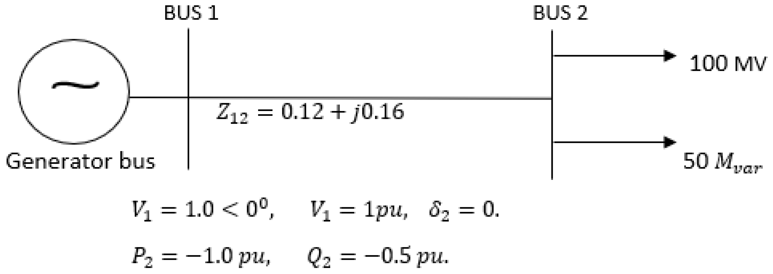
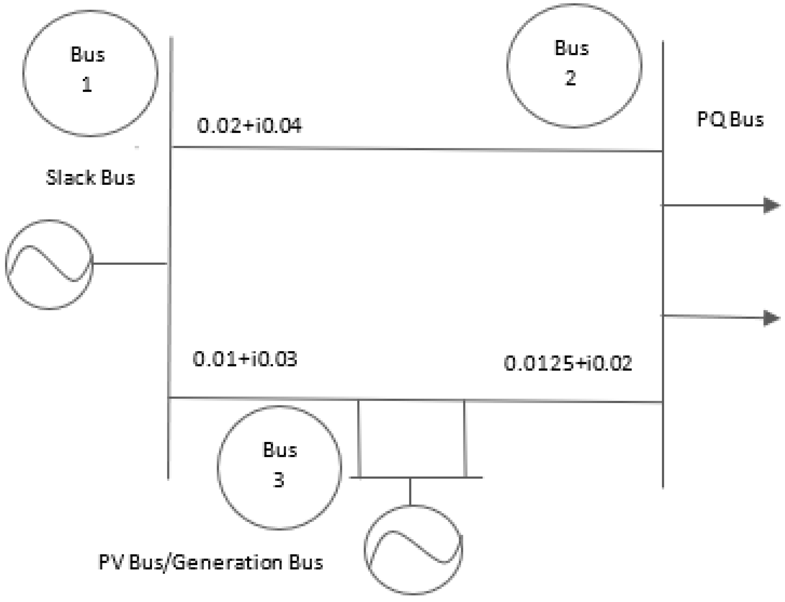
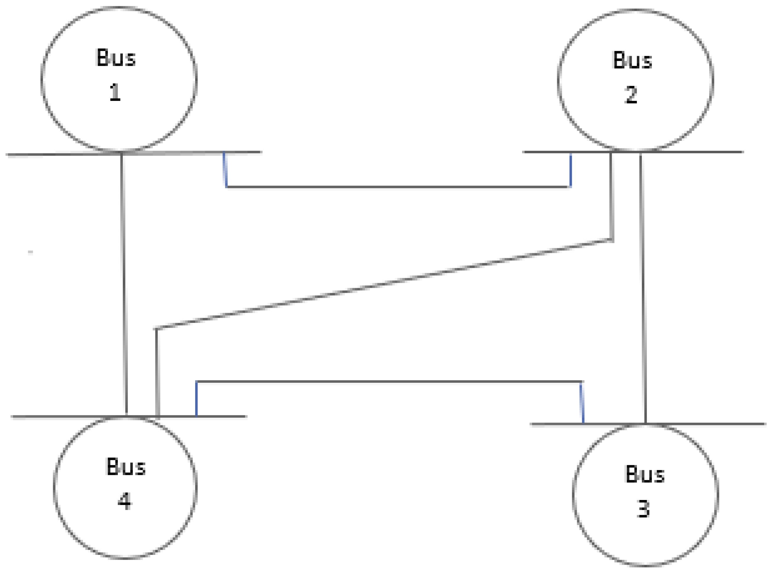
Formation of Load Flow Equations

In terms of the real power $\left(P\right)$, reactive power $\left(Q\right)$, and the voltage $\left(V\right)$, the general power flow equation is as follows:

$$S_i=P_i+j{Q}_i,$$

(25)

where $P_i$ represents real power injection, $Q_i$ represents reactive power injection, and $S_i$ is the complex power injection into the ith bus from the generating source. Thus,

$$S_i=P_i+j{Q}_i=V_i{I}_i^{*},$$

(26)

with

$$I_i^{*}={(\sum _{k=1}^n{Y}_{jk}{V}_k)}^{*},\mathrm{and}{I}^{*}={\left(\overline{I}\right)}^t.$$

By taking the complex conjugate of Equation (26), we obtain

$$S_i^{*}=P_i-j{Q}_i=V_i^{*}{I}_i=V_i^{*}\sum _{k=1}^n{Y}_{ik}{V}_k,i=1,2,\dots ,k.$$

(27)

In polar coordinate system, the Equation (27) for ith bus is described as

$$S_i^{*}=P_i-j{Q}_i=(V_i\angle -{\delta }_i)\sum _{k=1}^n(Y_{ik}\angle {\theta }_{ik})(V_k\angle {\delta }_k),$$

$$S_i^{*}=\sum _{k=1}^n\mid V_i{V}_k{Y}_{jk}\mid \angle ({\theta }_{ik}+{\delta }_k-{\delta }_i).$$

Now, for real power $P_i$ of ith bus, we have

$$P_i=\sum _{k=1}^n\mid V_i{V}_k{Y}_{jk}\mid cos({\theta }_{ik}+{\delta }_k-{\delta }_i).$$

(28)

Similarly, for the reactive power $Q_i$ of ith bus, we have

$$Q_i=-\sum _{k=1}^n\mid V_i{V}_k{Y}_{jk}\mid sin({\theta }_{ik}+{\delta }_k-{\delta }_i).$$

(29)

Therefore,

$$P_i=V_i{V}_i{Y}_{ii}cos\left({\theta }_{ii}\right)+\sum _{\begin{array}{c}k=1\\ k\ne i\end{array}}^n\mid V_i{V}_k{Y}_{ik}\mid cos({\theta }_{ik}+{\delta }_k-{\delta }_i).$$

(30)

and

$$Q_i=-V_i{V}_i{Y}_{ii}sin\left({\theta }_{ii}\right)-\sum _{\begin{array}{c}k=1\\ k\ne i\end{array}}^n\mid V_i{V}_k{Y}_{ik}\mid sin({\theta }_{ik}+{\delta }_k-{\delta }_i).$$

(31)

Four quantities at each bus are involved in order to solve the power flow equations, i.e., the real power $P_i,$ reactive power $Q_i,$ voltage $V_i$, and phase angle ${\delta }_i.$

$$P_i=g_1(\delta ,V)\mathrm{and}{Q}_i=g_2(\delta ,V).$$

We suppose that

$$\begin{array}{ccc}\hfill \mathsf{\Delta }{P}_i& =& P_i^s-P_i({\delta }_2,{\delta }_3,\dots ,{\delta }_k,V_2,V_3,\dots ,V_k),\hfill \\ \hfill \mathsf{\Delta }{Q}_i& =& Q_i^s-Q_i({\delta }_2,{\delta }_3,\dots ,{\delta }_k,V_2,V_3,\dots ,V_k),\hfill \end{array}$$

where $P_i^s$ and $Q_i^s$ are the defined values of $P_i$ and $Q_i$, respectively. By taking partial derivatives of $P_i$ and $Q_i$ with respect to ${\delta }_j$ and $V_j,$ we obtain

$$\begin{array}{ccc}\hfill \frac{\partial \mathsf{\Delta }{P}_i}{\partial {\delta }_j}& =& \frac{\partial (P_i^s-P_i(\delta ,V))}{\partial {\delta }_j}=-\frac{\partial P_i}{\partial {\delta }_j}\hfill \\ \hfill \frac{\partial \mathsf{\Delta }{P}_i}{\partial V_j}& =& -\frac{\partial P_i}{\partial V_j}.\hfill \end{array}$$

Similarly,

$$\begin{array}{ccc}\hfill \frac{\partial \mathsf{\Delta }{Q}_i}{\partial {\delta }_j}& =& \frac{\partial (Q_i^s-Q_i(\delta ,V))}{\partial {\delta }_j}=-\frac{\partial Q_i}{\partial {\delta }_j}\hfill \\ \hfill \frac{\partial \mathsf{\Delta }{Q}_i}{\partial V_j}& =& -\frac{\partial Q_i}{\partial V_j}.\hfill \end{array}$$

The Jacobian matrix is partitioned into the submatrices indicated below:

$$J=\left[\begin{array}{cc}{J}_{11}& J_{12}\\ J_{21}& J_{22}\end{array}\right].$$

$$\left[\begin{array}{c}\mathsf{\Delta }P\\ \mathsf{\Delta }Q\end{array}\right]=\left[\begin{array}{cc}{J}_{11}& J_{12}\\ J_{21}& J_{22}\end{array}\right]\left[\begin{array}{c}\mathsf{\Delta }\delta \\ \mathsf{\Delta }V\end{array}\right],$$

where

$$\mathsf{\Delta }\delta =\left[\begin{array}{c}\mathsf{\Delta }{\delta }_2\\ \mathsf{\Delta }{\delta }_3\\ ⋮\\ \mathsf{\Delta }{\delta }_n\end{array}\right],\mathsf{\Delta }V=\left[\begin{array}{c}\mathsf{\Delta }{V}_2\\ \mathsf{\Delta }{V}_3\\ ⋮\\ \mathsf{\Delta }{V}_n\end{array}\right],\mathsf{\Delta }P=\left[\begin{array}{c}\mathsf{\Delta }{P}_2\\ \mathsf{\Delta }{P}_3\\ ⋮\\ \mathsf{\Delta }{P}_n\end{array}\right],\mathsf{\Delta }Q=\left[\begin{array}{c}\mathsf{\Delta }{Q}_2\\ \mathsf{\Delta }{Q}_3\\ ⋮\\ \mathsf{\Delta }{Q}_n\end{array}\right].$$

The off-diagonal and diagonal elements of Jacobian submatrices are obtained by taking the partial derivatives of Equations (28) and (29) with respect to V and $\delta .$

$$J_{11}=\frac{\partial P}{\partial \delta }, J_{12}=\frac{\partial P}{\partial V}, J_{21}=\frac{\partial Q}{\partial \delta }, J_{22}=\frac{\partial Q}{\partial V}.$$

Example 1.

Suppose we have a two-bus power system as shown in the Figure 1. Bus 1 is taken as slack bus having ${\delta }_1=0,$ $\left|V_1\right|=1.0pu$, and Bus 2 is a load bus with $P_2=-1.0pu$, $Q_2=-0.5pu.$ A load of $100mw$ and $50Mvar$ is taken for Bus 2. The line impedance is $Z_{12}=0.12+j0.16pu$. Let us suppose an initial estimate of voltage magnitude $\left|V_2\right|=1pu$ and phase angle ${\delta }_2=0$.

As the numbers of buses in this system are two, so $Y_{bus}$ can be written as

$$Y_{bus}=\left[\begin{array}{cc}{Y}_{11}& Y_{12}\\ Y_{21}& Y_{22}\end{array}\right],$$

$$Y_{bus}=\left[\begin{array}{cc}5\angle -{53.13}^0& 5\angle {126.87}^0\\ 5\angle {126.87}^0& 5\angle -{53.13}^0\end{array}\right].$$

By expanding power flow equations, (28) and (29) for $n=2$, we obtain

$$P_2=V_2\sum _{k=1}^2{Y}_{2k}{V}_{k}cos({\theta }_{2k}+{\delta }_k-{\delta }_2),$$

(32)

$$Q_2=-V_2\sum _{k=1}^2{Y}_{2k}sin({\theta }_{2k}+{\delta }_k-{\delta }_2).$$

(33)

A $2\times 2$ system of nonlinear equations is obtained by substituting values of $Y_{bus}$ in Equations (32) and (33):

$$P_2=5V_{2}cos({126.87}^0-{\delta }_2)+5V_2^{2}cos(-{53.13}^0),$$

$$Q_2=-5V_{2}sin({126.87}^0-{\delta }_2)-5V_2^{2}sin(-{53.13}^0).$$

The initial guess is taken as $X^{\left(0\right)}={(1,1)}^t.$

Numerical results are shown in Table 4.

Table 4. Comparison of seventh-order schemes for load flow problem.

$\mathit{Cases}$	k	${\mathbf{\Vert }{\mathit{X}}^{\mathbf{\left(}\mathit{k}\mathbf{\right)}}\mathbf{-}{\mathit{X}}^{\mathbf{(}\mathit{k}\mathbf{-}\mathbf{1}\mathbf{)}}\mathbf{\Vert }}_{\mathbf{\infty }}$	${\mathbf{\Vert }\mathit{F}\mathbf{\left(}{\mathit{X}}^{\mathbf{\left(}\mathit{k}\mathbf{\right)}}\mathbf{\right)}\mathbf{\Vert }}_{\mathbf{\infty }}$	${\mathit{t}}^{\mathbf{\left(}\mathit{k}\mathbf{\right)}}$
$H{M}_1$	1	$9.89838070 (-1)$	$4.78059596 (-2)$
	2	$1.01619291 (-2)$	$2.07001814 (-12)$
	3	$4.43800774 (-13)$	$4.21224910 (-55)$	$1.353641$
$H{M}_2$	1	$9.90403466$	$4.447803895 (-2)$
	2	$9.59653379 (-3)$	$6.44704740 (-13)$
	3	$6.71636130 (-5)$	$1.84188372 (-43)$	$1.409686$
$H{M}_3$	1	$9.86538347 (-1)$	$6.33730798 (-2)$
	2	$1.34616521 (-2)$	$8.90751822 (-12)$
	3	$1.91374962 (-12)$	$1.49111311 (-56)$	$2.496505$
$S{F}_1$	1	$9.82754355 (-1)$	$8.02911898 (-2)$
	2	$1.724564463 (-2)$	$7.46401068 (-11)$
	3	$1.62714696 (-11)$	$4.50928147 (-54)$	$1.454692$
$S{F}_2$	1	$9.84331415 (-1)$	$7.30705632 (-2)$
	2	$1.56685847 (-2)$	$1.70343570 (-11)$
	3	$3.70209774 (-12)$	$2.20545208 (-55)$	$1.40545$

Table 4. Comparison of seventh-order schemes for load flow problem.

$\mathit{Cases}$	k	${\mathbf{\Vert }{\mathit{X}}^{\mathbf{\left(}\mathit{k}\mathbf{\right)}}\mathbf{-}{\mathit{X}}^{\mathbf{(}\mathit{k}\mathbf{-}\mathbf{1}\mathbf{)}}\mathbf{\Vert }}_{\mathbf{\infty }}$	${\mathbf{\Vert }\mathit{F}\mathbf{\left(}{\mathit{X}}^{\mathbf{\left(}\mathit{k}\mathbf{\right)}}\mathbf{\right)}\mathbf{\Vert }}_{\mathbf{\infty }}$	${\mathit{t}}^{\mathbf{\left(}\mathit{k}\mathbf{\right)}}$
$H{M}_1$	1	$9.89838070 (-1)$	$4.78059596 (-2)$
	2	$1.01619291 (-2)$	$2.07001814 (-12)$
	3	$4.43800774 (-13)$	$4.21224910 (-55)$	$1.353641$
$H{M}_2$	1	$9.90403466$	$4.447803895 (-2)$
	2	$9.59653379 (-3)$	$6.44704740 (-13)$
	3	$6.71636130 (-5)$	$1.84188372 (-43)$	$1.409686$
$H{M}_3$	1	$9.86538347 (-1)$	$6.33730798 (-2)$
	2	$1.34616521 (-2)$	$8.90751822 (-12)$
	3	$1.91374962 (-12)$	$1.49111311 (-56)$	$2.496505$
$S{F}_1$	1	$9.82754355 (-1)$	$8.02911898 (-2)$
	2	$1.724564463 (-2)$	$7.46401068 (-11)$
	3	$1.62714696 (-11)$	$4.50928147 (-54)$	$1.454692$
$S{F}_2$	1	$9.84331415 (-1)$	$7.30705632 (-2)$
	2	$1.56685847 (-2)$	$1.70343570 (-11)$
	3	$3.70209774 (-12)$	$2.20545208 (-55)$	$1.40545$

It can be noted from Table 4, that our method $H{M}_1$ dominates all the methods in terms of less error and less computational time.

Example 2.

Consider a general three-bus power system [6]. Bus 1 is considered as a slack bus with voltage magnitude $\left|V_1\right|=1.05pu$, Bus 2 is a $PQ$ bus with a load of $P_2=-4.0pu$ and $Q_2=-2.5pu$, and Bus 3 is a generation bus having magnitude of voltage as $\left|V_3\right|=1.04pu$ and $P_3=2.0pu$. The impedances are shown in Figure 2.

$Y_{bus}$ matrix for this system is written as

$$Y_{bus}=\left[\begin{array}{ccc}{Y}_{11}& Y_{12}& Y_{13}\\ Y_{21}& Y_{22}& Y_{23}\\ Y_{31}& Y_{32}& Y_{33}\end{array}\right],$$

$$\left|Y_{bus}\right|=\left[\begin{array}{ccc}53.8516& 22.3606& 31.6228\\ 22.3606& 58.1378& 35.7771\\ 31.6228& 35.7771& 67.2309\end{array}\right]\mathrm{and}\left|Y_{{\theta }_{Bus}}\right|=\left[\begin{array}{ccc}68.1986& 116.5651& 108.4349\\ 116.5651& 63.4349& 116.5651\\ 108.4349& 116.5631& 67.2490\end{array}\right].$$

Thus, in this case, $Y_{Bus}$ admittance matrix is

$$Y_{bus}=\left[\begin{array}{ccc}53.8516\angle -{68.1986}^0& 22.3606\angle {116.5651}^0& 31.6228\angle {108.4349}^0\\ 22.3606\angle {116.5651}^0& 58.1378\angle -{63.4349}^0& 35.7771\angle {116.5651}^0\\ 31.6228\angle {108.4349}^0& 35.7771\angle {116.5631}^0& 67.2309\angle -{67.2490}^0\end{array}\right].$$

For $n=3$, the power flow Equations (28) and (29) for the unknowns, i.e., $P_2,P_3$, and $Q_2$, can be written as

$$P_2=V_2\sum _{k=1}^3{Y}_{2k}{V}_{k}cos({\theta }_{2k}+{\delta }_k-{\delta }_2),$$

(34)

$$P_3=V_3\sum _{k=1}^3{Y}_{3k}{V}_{k}cos({\theta }_{3k}+{\delta }_k-{\delta }_3),$$

(35)

$$Q_2=-V_2\sum _{k=1}^3{Y}_{2k}{V}_{k}sin({\theta }_{2k}+{\delta }_k-{\delta }_2).$$

(36)

A $3\times 3$ nonlinear system of equations is obtained by substituting the values in (34)–(36):

$$P_2=23.478630V_{2}cos(-2.03444+{\delta }_2)+26.00005V_2^2+37.20818V_{2}cos(-2.0344-{\delta }_3+{\delta }_2)+4,$$

$$P_3=34.53209cos(-1.89254+{\delta }_3)+37.208184V_{2}cos(2.034444788-{\delta }_3+{\delta }_2)+26.12160874,$$

$$Q_2=23.478630V_{2}sin(-2.03444+{\delta }_2)+52.0000V_2^2+37.20818V_{2}sin(-2.034444788-{\delta }_3+{\delta }_2)+2.5.$$

The required solution for the system of nonlinear equations for our problem is $X={(-2.6964802629,-0.4988374911,0.9716777891)}^t$ and the initial guess is taken as $X^{\left(0\right)}={(0,0,1)}^t.$

Numerical results are shown in the following Table 5.

Table 5. Comparison of seventh-order schemes for power flow problem.

$\mathit{Cases}$	k	${\mathbf{\Vert }{\mathit{X}}^{\mathbf{\left(}\mathit{k}\mathbf{\right)}}\mathbf{-}{\mathit{X}}^{\mathbf{(}\mathit{k}\mathbf{-}\mathbf{1}\mathbf{)}}\mathbf{\Vert }}_{\mathbf{\infty }}$	${\mathbf{\Vert }\mathit{F}\mathbf{\left(}{\mathit{X}}^{\mathbf{\left(}\mathit{k}\mathbf{\right)}}\mathbf{\right)}\mathbf{\Vert }}_{\mathbf{\infty }}$	${\mathit{t}}^{\mathbf{\left(}\mathit{k}\mathbf{\right)}}$
$H{M}_1$	1	$4.7062458908 (-2)$	$2.9429422347 (-6)$
	2	$5.3524284668 (-8)$	$1.8153562097 (-36)$
	3	$3.35876206 (-38)$	$2.84164745 (-47)$	$1.987282$
$H{M}_2$	1	$4.7062482460 (-2)$	$3.0040159229 (-6)$
	2	$4.1730381388 (-8)$	$2.1707785791 (-36)$
	3	$3.49657037 (-38)$	$2.84164745 (-47)$	$1.972989$
$H{M}_3$	1	$4.7062549068 (-2)$	$8.0832420909 (-6)$
	2	$9.0817922071 (-8)$	$3.6267951935 (-34)$
	3	$6.02690441 (-36)$	$2.84164745 (-47)$	$1.963466$
$S{F}_1$	1	$4.70624694 (-2)$	$1.46430173 (-6)$
	2	$2.63918687 (-8)$	$2.26013119 (-38)$
	3	$3.73850774 (-40)$	$2.84164745 (-47)$	$2.006422$
$S{F}_2$	1	$4.70624886 (-2)$	$7.32584352 (-7)$
	2	$2.71328333 (-8)$	$3.11954284 (-38)$
	3	$7.52218608 (-40)$	$2.84164745 (-47)$	$2.003059$

Table 5. Comparison of seventh-order schemes for power flow problem.

$\mathit{Cases}$	k	${\mathbf{\Vert }{\mathit{X}}^{\mathbf{\left(}\mathit{k}\mathbf{\right)}}\mathbf{-}{\mathit{X}}^{\mathbf{(}\mathit{k}\mathbf{-}\mathbf{1}\mathbf{)}}\mathbf{\Vert }}_{\mathbf{\infty }}$	${\mathbf{\Vert }\mathit{F}\mathbf{\left(}{\mathit{X}}^{\mathbf{\left(}\mathit{k}\mathbf{\right)}}\mathbf{\right)}\mathbf{\Vert }}_{\mathbf{\infty }}$	${\mathit{t}}^{\mathbf{\left(}\mathit{k}\mathbf{\right)}}$
$H{M}_1$	1	$4.7062458908 (-2)$	$2.9429422347 (-6)$
	2	$5.3524284668 (-8)$	$1.8153562097 (-36)$
	3	$3.35876206 (-38)$	$2.84164745 (-47)$	$1.987282$
$H{M}_2$	1	$4.7062482460 (-2)$	$3.0040159229 (-6)$
	2	$4.1730381388 (-8)$	$2.1707785791 (-36)$
	3	$3.49657037 (-38)$	$2.84164745 (-47)$	$1.972989$
$H{M}_3$	1	$4.7062549068 (-2)$	$8.0832420909 (-6)$
	2	$9.0817922071 (-8)$	$3.6267951935 (-34)$
	3	$6.02690441 (-36)$	$2.84164745 (-47)$	$1.963466$
$S{F}_1$	1	$4.70624694 (-2)$	$1.46430173 (-6)$
	2	$2.63918687 (-8)$	$2.26013119 (-38)$
	3	$3.73850774 (-40)$	$2.84164745 (-47)$	$2.006422$
$S{F}_2$	1	$4.70624886 (-2)$	$7.32584352 (-7)$
	2	$2.71328333 (-8)$	$3.11954284 (-38)$
	3	$7.52218608 (-40)$	$2.84164745 (-47)$	$2.003059$

As observed from Table 5, the newly proposed methods are relatively efficient in terms of error while we also observe mere difference in terms of computational time.

Example 3.

Consider a general four-bus power system as shown in the Figure 3; Bus 1 is considered as a slack bus with voltage magnitude $\left|V_1\right|=1.04pu$, ${\delta }_1=0.$ Bus 2 and Bus 3 are PQ buses, while Bus 4 is a slack bus. The magnitude of voltage is $\left|V_4\right|=1.0pu$, ${\delta }_4=0,$ $P_2=0.5pu$, $Q_2=0.208pu$ and $P_3=-1.0pu$, $Q_3=0.5pu$.

$Y_{bus}$ matrix for this system is written as

$$Y_{bus}=\left[\begin{array}{cccc}{Y}_{11}& Y_{12}& Y_{13}& Y_{14}\\ Y_{21}& Y_{22}& Y_{23}& Y_{24}\\ Y_{31}& Y_{32}& Y_{33}& Y_{34}\\ Y_{41}& Y_{42}& Y_{43}& Y_{44}\end{array}\right],$$

$$\left|Y_{bus}\right|=\left[\begin{array}{cccc}9.486833& 6.324555& 3.162277& 0\\ 6.324555& 11.594807& 2.107974& 3.162277\\ 3.162277& 2.107974& 11.594807& 6.324555\\ 0& 3.162277& 6.324555& 9.486833\end{array}\right]$$

and

$$\left|Y_{{\theta }_{Bus}}\right|=\left[\begin{array}{cccc}-71.565051& -68.423458& -68.423458& 0\\ -68.423458& -71.568176& -68.440648& -68.423458\\ -68.423458& -68.440648& -71.568176& -68.423458\\ 0& -68.423458& -68.423458& -71.565051\end{array}\right].$$

Thus, in this case, the $Y_{Bus}$ admittance matrix is

$$Y_{bus}=\left[\begin{array}{cccc}3.0-j9.0& -2.0+j6.0& -1.0+j3.0& 0\\ -2.0+j6.0& 3.666-j11.0& -0.666+j2.0& -1.0+j3.0\\ -1.0+j3.0& -0.666+j2.0& 3.666-j11.0& -2.0+j6.0\\ 0& -1.0+j3.0& -2.0+j6.0& 3.0-j9.0\end{array}\right].$$

For $n=4$, the power flow Equations (28) and (29) for the unknowns, i.e., $P_2$, $P_3,Q_2$ and $Q_3$, can be written as

$$P_2=V_2\sum _{k=1}^4{Y}_{2k}{V}_{k}cos({\theta }_{2k}+{\delta }_k-{\delta }_2),$$

(37)

$$P_3=V_3\sum _{k=1}^4{Y}_{3k}{V}_{k}cos({\theta }_{3k}+{\delta }_k-{\delta }_3),$$

(38)

$$Q_2=-V_2\sum _{k=1}^4{Y}_{2k}{V}_{k}sin({\theta }_{2k}+{\delta }_k-{\delta }_2),$$

(39)

$$Q_3=-V_3\sum _{k=1}^4{Y}_{3k}{V}_{k}sin({\theta }_{3k}+{\delta }_k-{\delta }_3).$$

(40)

A $4\times 4$ nonlinear system of equations is obtained by substituting the values in (37)–(40):

$$\begin{array}{ccc}\hfill P_2& =& 6.577537V_{2}cos(-68.423458-{\delta }_2)+3.665999V_2^2\hfill \\ & & +2.107974V_2{V}_{3}cos(-68.440649+{\delta }_3-{\delta }_2)+3.162277V_{2}cos(-68.423458-{\delta }_2),\hfill \end{array}$$

$$\begin{array}{ccc}\hfill P_3& =& 3.288768V_{3}cos(-68.423458-{\delta }_3)+2.107974V_2{V}_{3}cos(-68.440649+{\delta }_2-{\delta }_3)\hfill \\ & & +3.665999V_3^2+6.324555V_{3}cos(-68.423458-{\delta }_3),\hfill \end{array}$$

$$\begin{array}{ccc}\hfill Q_2& =& -6.577537V_{2}sin(-68.423458-{\delta }_2)+10.999999V_2^2\hfill \\ & & -2.107974V_2{V}_{3}sin(-68.440649+{\delta }_3-{\delta }_2)-3.162277V_{2}sin(-68.423458-{\delta }_2),\hfill \end{array}$$

$$\begin{array}{ccc}\hfill Q_3& =& -3.288768V_{3}sin(-68.423458-{\delta }_3)-2.107974V_2{V}_{3}sin(-68.440649+{\delta }_2-{\delta }_3)\hfill \\ & & +10.999999V_3^2-6.324555V_{3}sin(-68.423458-{\delta }_3).\hfill \end{array}$$

The initial guess is taken as $X^{\left(0\right)}={(0.4,0.4,0,0)}^t.$

Numerical results are shown in the following Table 6.

Table 6. Comparison of seventh-order schemes for power flow problem.

$\mathit{Cases}$	k	${\mathbf{\Vert }{\mathit{X}}^{\mathbf{\left(}\mathit{k}\mathbf{\right)}}\mathbf{-}{\mathit{X}}^{\mathbf{(}\mathit{k}\mathbf{-}\mathbf{1}\mathbf{)}}\mathbf{\Vert }}_{\mathbf{\infty }}$	${\mathbf{\Vert }\mathit{F}\mathbf{\left(}{\mathit{X}}^{\mathbf{\left(}\mathit{k}\mathbf{\right)}}\mathbf{\right)}\mathbf{\Vert }}_{\mathbf{\infty }}$	${\mathit{t}}^{\mathbf{\left(}\mathit{k}\mathbf{\right)}}$
$H{M}_1$	1	$3.9406592707102$	$5.585285030714$	$2.617419$
	2	$2.3539462998374$	$1.185340119973$
	3	$3.93041986150 (-1)$	$2.70471496585 (-2)$
$H{M}_2$	1	$1.12028592195 (+1)$	$1.69904638491$	$2.672200$
	2	$6.059912678220$	$4.67290040442 (+2)$
	3	$5.615825776275$	$7.552107353633$
$H{M}_3$	1	$1.153695471270$	$3.35717069246 (-1)$	$2.561838$
	2	$3.77060518279 (-1)$	$3.22883832204 (-4)$
	3	$2.63676291247 (-4)$	$1.80483165050 (-20)$
$S{F}_1$	1	$1.2238519878510$	$1.0000236962$	$2.713051$
	2	$1.238095340437$	$4.5105399975 (-1)$
	3	$3.87777272650 (-1)$	$1.01937440334 (-3)$
$S{F}_2$	1	$1.80701993172$	$1.78530748656$	$2.898047$
	2	$6.23700907210$	$1.527984713366$
	3	$5.81002994904$	$1.277471753569$

Table 6. Comparison of seventh-order schemes for power flow problem.

$\mathit{Cases}$	k	${\mathbf{\Vert }{\mathit{X}}^{\mathbf{\left(}\mathit{k}\mathbf{\right)}}\mathbf{-}{\mathit{X}}^{\mathbf{(}\mathit{k}\mathbf{-}\mathbf{1}\mathbf{)}}\mathbf{\Vert }}_{\mathbf{\infty }}$	${\mathbf{\Vert }\mathit{F}\mathbf{\left(}{\mathit{X}}^{\mathbf{\left(}\mathit{k}\mathbf{\right)}}\mathbf{\right)}\mathbf{\Vert }}_{\mathbf{\infty }}$	${\mathit{t}}^{\mathbf{\left(}\mathit{k}\mathbf{\right)}}$
$H{M}_1$	1	$3.9406592707102$	$5.585285030714$	$2.617419$
	2	$2.3539462998374$	$1.185340119973$
	3	$3.93041986150 (-1)$	$2.70471496585 (-2)$
$H{M}_2$	1	$1.12028592195 (+1)$	$1.69904638491$	$2.672200$
	2	$6.059912678220$	$4.67290040442 (+2)$
	3	$5.615825776275$	$7.552107353633$
$H{M}_3$	1	$1.153695471270$	$3.35717069246 (-1)$	$2.561838$
	2	$3.77060518279 (-1)$	$3.22883832204 (-4)$
	3	$2.63676291247 (-4)$	$1.80483165050 (-20)$
$S{F}_1$	1	$1.2238519878510$	$1.0000236962$	$2.713051$
	2	$1.238095340437$	$4.5105399975 (-1)$
	3	$3.87777272650 (-1)$	$1.01937440334 (-3)$
$S{F}_2$	1	$1.80701993172$	$1.78530748656$	$2.898047$
	2	$6.23700907210$	$1.527984713366$
	3	$5.81002994904$	$1.277471753569$

Table 6 shows that $H{M}_3$ is working exceptionally well in terms of less error and less computational time. Moreover, the methods $H{M}_1$ and $H{M}_2$ also use less computational time in the three iterations. It is pertinent to mention that to acquire accuracy similar to $H{M}_3$, the methods $H{M}_2$ and $S{F}_2$ need 27 more iterations.

4. Concluding Remarks

We introduced a new efficient three-step seventh-order scheme to obtain the solutions of nonlinear system of equations. The computational cost for different operations is expressed and is used to calculate the cost of our proposed method, and is compared with the cost of some existing seventh-order methods. The applicability of our scheme is interpreted in an electrical power system, and two-bus, three-bus, and four-bus power flow problems are solved by using load flow equations. In all the examples, we observe that the newly proposed methods are offering less computational time even when the number of buses increases. Moreover, our class of iterative schemes has only one inverse operator. Thus, by using the LU factorization for the linear systems involved per iteration, the computational cost is reduced, even for large systems in relation to other schemes with more than one inverse operator. Overall, we conclude that the higher-order Jarratt-type methods provide a valuable alternative for solving load flow equations in power system analysis, offering faster convergence, improved accuracy, and enhanced stability, particularly in the context of highly nonlinear power systems. In addition, one of the main drawbacks of these techniques is the J matrix singularity, due to which the methods are sometimes unable to produce the solution. The cause could be anything from a sudden big load addition or subtraction to a change in the line characteristics to an overvoltage or undervoltage at a specific bus. These demerits may be handled by combining the higher-order Jarratt methods and evolutionary/intelligent algorithms.

References

1. Jarratt, P. Some efficient fourth order multipoint methods for solving equations. BIT Numer. Math. 1969, 9, 119–124. [Google Scholar] [CrossRef]
2. Behl, R.; Sarría, Í.; González, R.; Magreñán, Á.A. Highly efficient family of iterative methods for solving nonlinear models. J. Comput. Appl. Math. 2019, 346, 110–132. [Google Scholar] [CrossRef]
3. Hueso, J.L.; Martínez, E.; Teruel, C. Convergence, efficiency and dynamics of new fourth and sixth order families of iterative methods for nonlinear systems. J. Comput. Appl. Math. 2015, 275, 412–420. [Google Scholar] [CrossRef]
4. Lee, M.Y.; Kim, Y.I. Development of a Family of Jarratt-Like Sixth-Order Iterative Methods for Solving Nonlinear Systems with Their Basins of Attraction. Algorithms 2020, 13, 303. [Google Scholar] [CrossRef]
5. Abad, M.; Cordero, A.; Torregrosa, J.R. A family of seventh-order schemes for solving nonlinear systems. Bull. Math. Soc. Sci. Math. 2014, 57, 133–145. [Google Scholar]
6. Yaseen, S.; Zafar, F.; Chicharro, F.I. A seventh order family of Jarratt type iterative method for electrical power systems. Fractal Fract. 2023, 7, 317. [Google Scholar] [CrossRef]
7. Narang, M.; Bhatia, S.; Kanwar, V. New efficient derivative free family of seventh-order methods for solving systems of nonlinear equations. Numer. Algorithms 2017, 76, 283–307. [Google Scholar] [CrossRef]
8. Sharma, J.R.; Arora, H. A novel derivative free algorithm with seventh order convergence for solving systems of nonlinear equations. Numer. Algorithms 2014, 67, 917–933. [Google Scholar] [CrossRef]
9. Sharma, J.R.; Arora, H. A simple yet efficient derivative free family of seventh order methods for systems of nonlinear equations. SeMA J. 2016, 73, 59–75. [Google Scholar] [CrossRef]
10. Wang, X.; Zhang, T. A family of Steffensen type methods with seventh-order convergence. Numer. Algorithms 2013, 62, 429–444. [Google Scholar] [CrossRef]
11. Wang, X.; Zhang, T.; Qian, W.; Teng, M. Seventh-order derivative-free iterative method for solving nonlinear systems. Numer. Algorithms 2015, 70, 545–558. [Google Scholar] [CrossRef]
12. Behl, R.; Arora, H. CMMSE: A novel scheme having seventh-order convergence for nonlinear systems. J. Comput. Appl. Math. 2022, 404, 113301. [Google Scholar] [CrossRef]
13. Wang, X. Fixed-point iterative method with eighth-order constructed by undetermined parameter technique for solving nonlinear systems. Symmetry 2021, 13, 863. [Google Scholar] [CrossRef]
14. Xiao, X.Y. New techniques to develop higher order iterative methods for systems of nonlinear equations. Comp. Appl. Math. 2022, 41, 243. [Google Scholar] [CrossRef]
15. Zhanlav, T.; Otgondorj, K. Higher order Jarratt-like iterations for solving systems of nonlinear equations. Appl. Math. Comput. 2021, 395, 125849. [Google Scholar] [CrossRef]
16. Zhanlav, T.; Mijiddorj, R.; Otgondorj, K. A family of Newton-type methods with seventh and eighth-order of convergence for solving systems of nonlinear equations. Hacettepe J. Math. Stat. 2023, 52, 1006–1021. [Google Scholar] [CrossRef]
17. Sharma, J.R.; Guha, R.K.; Sharma, R. An efficient fourth order weighted-Newton method for systems of nonlinear equations. Numer. Algorithms 2013, 62, 307–323. [Google Scholar] [CrossRef]
18. Bergen, A.R. Power Systems Analysis; Pearson Education India: New Delhi, India, 2009. [Google Scholar]
19. Glover, J.D.; Overbye, T.J.; Sarma, M.S. Power System Analysis & Design; SI Version; Cengage Learning: Boston, MA, USA, 2015. [Google Scholar]
20. Nagsarkar, T.K.; Sukhija, M.S. Power System Analysis, 2nd ed.; Oxford University Press: New Delhi, India, 2014. [Google Scholar]
21. Saadat, H. Power System Analysis; The McGraw-Hill Companies, Inc.: New York, NY, USA, 2002. [Google Scholar]
22. Ward, J.B.; Hale, H.W. Digital computer solution of power flow problems. AIEE Trans. 1956, 75, 398–404. [Google Scholar]
Figure 1. Two-bus system.
Algorithms 17 00086 g001
Figure 2. Three-bus system.
Algorithms 17 00086 g002
Figure 3. Four-bus system.
Algorithms 17 00086 g003