Abstract
Solving combinatorial problems on complex networks represents a primary issue which, on a large scale, requires the use of heuristics and approximate algorithms. Recently, neural methods have been proposed in this context to find feasible solutions for relevant computational problems over graphs. However, such methods have some drawbacks: (1) they use the same neural architecture for different combinatorial problems without introducing customizations that reflects the specificity of each problem; (2) they only use a nodes local information to compute the solution; (3) they do not take advantage of common heuristics or exact algorithms. Following this interest, in this research we address these three main points by designing a customized attention-based mechanism that uses both local and global information from the adjacency matrix to find approximate solutions for the Minimum Vertex Cover Problem. We evaluate our proposal with respect to a fast two-factor approximation algorithm and a widely adopted state-of-the-art heuristic both on synthetically generated instances and on benchmark graphs with different scales. Experimental results demonstrate that, on the one hand, the proposed methodology is able to outperform both the two-factor approximation algorithm and the heuristic on the test datasets, scaling even better than the heuristic with harder instances and, on the other hand, is able to provide a representation of the nodes which reflects the combinatorial structure of the problem.
1. Overview
Combinatorial issues that deal with network optimization problems have motivated several branches of computational science, also thanks to the huge real-world contexts in which they find application (e.g., bioinformatics [1], sensor networks [2], biology [3], information retrieval [4] and, more recently, natural language processing [5]). Most of these problems are intractable (NP-hard). Minimum Vertex Cover (MVC) or its weighted version (MWVC) [6,7,8], Maximum Clique (MC) [9,10] or Traveling Salesman (TS) [11,12] are notable examples of NP-hard problems [13] over graphs for which various approximation algorithms or heuristics solvers have been proposed as effective alternatives to exact exponential methods [14,15].
In recent years, the use of Deep-Learning (DL) approaches has been proposed for solving NP-hard problems over graphs in a purely data-driven fashion. Among these, the most notable are Pointer Networks [16] and Neural Networks with Dynamic External Memory [17].These approaches are classical end-to-end learning frameworks based on the usage of neural networks extended with recent DL mechanisms such as neural attention or external memory. Nevertheless, the general DL architectures and the strictly data-driven learning approaches proposed in these pioneering works have been criticized for being too generic and for not considering the peculiarity of different graph problems [18], thus not providing theoretical guarantees. More effective research investigation directions are based on using Reinforcement Learning (RL) [18,19,20,21,22] or Graph Neural Networks (GNNs) [23,24] not in an end-to-end fashion, but with a two-stage approach: a first stage in which they learn a representation of the graph (with DL techniques like GNNs, in a representation learning fashion), and a second stage in which this representation is used to build the solution to the combinatorial optimization problem using an autoregressive machine-learning-based procedure (e.g., with RL), or using greedy algorithms or local search. It has been shown that representation learning-based approaches are better in building solutions to combinatorial optimization over graphs with respect to end-to-end approaches, but the majority of the proposed research shares some drawbacks [25,26]:
- In many graph-based combinatorial optimization problems, the global information of the graph is needed for solving the problem; however, existing graph learning models, especially GNN, only aggregate local information from neighbors. Roughly speaking, this is because GNNs are based on the neural message-passing framework, i.e., to build node representations, they follow an iterative schema of updating node representations based on the aggregation from nearby nodes. The role of the aggregation function is to aggregate information from its neighborhood and pass on the information to the next layer. More global information can be obtained by adding more message-passing layers; however, this can cause over-smoothing, a non-trivial phenomenon according to which, after several iterations of GNN message passing, the representations for all the nodes in the graph can become very similar to one another. Therefore, neural message-passing iterations are generally kept low, thus not effectively encoding global information of graphs.
- General DL architectures are used to solve different types of combinatorial optimization problems (MVC, TS, MC); however, each problem has its own characteristics and constraints. Encoding inductive bias into DL architectures to better capture the characteristics of the combinatorial optimization problem is often missing.
- Many approaches do not integrate or take into account traditional heuristics even though identifying the operations of traditional heuristics of a combinatorial optimization problem and integrating such operations appropriately into the learning procedure or in the methodology can benefit the learning-based methods.
In this paper, we focus on the MVC problem, a traditional NP-hard optimization problem of finding the minimum sized subset of nodes of an undirected graph such that every edge in G has at least one endpoint in . The interest in the MVC problem is motivated by its many real-world applications and by its recent extension to the less explored context of temporal networks [27]. Theoretical analyses indicate that the MVC problem is NP-hard and the associated decision problem is NP-complete [13]. Moreover, it is NP-hard to approximate MVC within any factor smaller than for any assuming [28] and within constant factor smaller than two assuming the Unique Game Conjecture [29], although an approximation ratio of has been proposed [30]. Despite this, MVC has several simple 2-factor approximations: e.g., in [31], where the authors propose a local-ratio algorithm for computing an approximate vertex cover; the algorithm greedily reduces the costs over edges, iteratively building a cover. The worst-case runtime of this implementation is , where n is the number of nodes and m the number of edges in the graph. An implementation of such an algorithm is available in [32]. If, on the one hand, 2-factor approximations are very useful for their low complexity, on the other hand, they produce results that are quite far from the optimum. Various exact algorithms or heuristic algorithms have been proposed to overcome this problem. Exact methods, which mainly include Integer Linear Programming (ILP) [33], branch-and-bound algorithms [34,35,36,37], and fixed-parameter tractable algorithms [38] guarantee the optimality of their solutions, but may fail to give a solution within reasonable time for large or medium-size instances. Heuristic algorithms, like NuMVC [39] and FastVC [40], which are mainly based on local search, cannot guarantee the optimality of their solutions, but they can find satisfactory near-optimal solutions for large and hard instances within reasonable time. These heuristic-based approaches have become state-of-the-art for many real-world use cases, and they have also inspired heuristic-based algorithms for the weighted version of the problem [41,42]. More recently, as for other combinatorial optimization problems over graphs, the research trend for MVC has moved towards the adoption of DL techniques with RL as in [21] or GNN as in [23]. However, these solutions suffer from the main drawbacks of other DL-based approaches for combinatorial optimization over graphs, i.e., they build graph representations considering only local information, they adopt general DL techniques without customizing them according to the nature of the specific combinatorial problem, and they do not take advantage of the state-of-the-art heuristics for such problem by integrating them into the learning methodology.
In this research, we propose a custom DL-based approach to solve the MVC problem by addressing these three main challenges: (1) build a suitable graph representation at the node level using both global and local information; (2) customize a common DL approach based on attention to reflect the combinatorial structure of MVC problems; (3) integrate the DL methodology with state-of-the-art heuristics to take advantage of them. The proposed approach, which we named Attention with Complement Information (ACI), is based on an encoder–decoder architecture that adopts the attention mechanism and a memory network to build node representation exploiting both the adjacency matrix and its complement. In this way, (1) an MVC-biased representation of the graph is built considering both local and global information, and (2) we adapt a common DL approach to the MVC problem. We also propose to use the representation obtained within a state-of-the-art heuristic to produce a final covering set, thus (3) taking advantage of it, also from a theoretical perspective.
Our experimental results suggest that the proposed methodology can learn suitable node representation for combinatorial problems. Indeed, on the one hand, we tested our models against a fast 2-factor approximation algorithm and a widely adopted state-of-the-art heuristic, showing that, on average, the methodology is able to outperform both the 2-factor approximation algorithm and the heuristic in finding a vertex cover of the smallest possible size, scaling well also with larger instances, from the other, we explore the representation capabilities of our approach with visual artifacts, providing evidence of the fact that the methodology is able to represent nodes reflecting the combinatorial structure of the problem.
The remainder of the paper is organized as follows: in Section 2, we provide the basic concepts from graph theory to understand the MVC problem, with a focus also on the attention mechanism and memory networks that have been adopted in the proposed solution. In Section 3, we provide the details of our methodology, and in Section 4, our experimental results are discussed together with training and test datasets, selected network hyperparameters, and evaluation metrics. Moreover, a discussion on the expressive power of the proposed methodology with respect to representation learning is reported; finally, Section 5 suggests some hints on future research directions.
2. Basic Concepts and Problem Definition
In this section, we first introduce basic concepts about graphs and the MVC problem; then, we introduce the basics of the DL techniques adopted in this research.
Definition 1 (Graph).
A Graph is a pair , where N is the set of nodes and E is the set of edges, such that each element of E is a pair of element of N.
An edge that links two nodes and can be denoted as . Moreover, if E is not a symmetric relation, the graph is said to be undirected, and if edges are not weighted, the graph is said to be unweighted. Since we focus on these kinds of graphs, in the following, we will generally refer to graphs as unweighted, undirected graphs.
At the node level, graphs can be represented by features that describe structural graph information. Node degree, i.e., the quantity of direct neighbors of a node (or the number of incident edges), is one of the most commonly used since it can naturally indicate the importance of a node within the graph. As for node-level description, graph-level features can be used. Among the most commonly used, density conceptually provides an idea of how much connected a graph is and is measured by the ratio between edges and nodes within a graph, . Another relevant concept is clique, i.e., a set of vertices, all pairs of which are adjacent.
Definition 2 (Minimum Vertex Cover).
Given an unweighted undirected graph , a vertex cover is a subset of . A minimum vertex cover is a vertex cover of the smallest possible size.
This problem can be formulated as the following integer linear program:
where the objective function consists of minimizing the number of nodes belonging to the covering set, such that every edge of the graph is covered () and every vertex is either in the vertex cover or not ().
With the above definitions we can state our objective as follows: Given an unweighted undirected graph , with N nodes and E edges and a minimum vertex cover of G, we want to find a parametric function which is able to map the input graph G to the set of covering nodes , .
The MVC problem does not have a unique optimal solution. The solution, i.e., the minimum covering set, mainly depends on the order according to which edges or nodes are scanned to determine whether they should be part of it.
As an example, a very simple approximated approach to solving the problem consists of starting from the set E of all edges, where edges are arbitrarily ordered (suppose, without loss of generality, that they are named with capital letters, and they are ordered lexicographically). The approach consists of iteratively scanning this set so that at each iteration, edge is picked, and nodes u and v are added to the final covering set . Then, all the other edges in E, which are either incident to u or v are removed. This is carried out until E is empty. represents the final solution. Figure 1 shows an example of this. By applying the described approach to the left-side graph, assuming that edges are ordered lexicographically since edge is the first scanned, the results would be . By changing the name of the edges (right-side graph) and applying the same procedure using the lexicographical order, the first scanned edge would be . Thus, the final result would be .
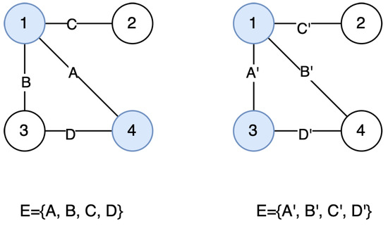
Figure 1.
Example of distinct optimal solutions for the same graph. Covering nodes are colored blue. On the left-hand graph, the optimal solution is composed of nodes 1 and 4; on the right-hand of nodes 1 and 3. The difference in the result is determined by the different way edges are ordered and picked to compute the final solution.
In general, iterative algorithms (either approximated or exact) do not pick edges or nodes completely at random, but they order them according to some heuristic or criterion as in [37,39,40]. However, it is clear that, according to these approaches, the order according to which edges are picked from the initial set highly influences the final result since the fact that a node is already part of the final solution has an impact on the fact that another node should be part of it. In our example in Figure 1, the fact that node 3 is already part of the solution implies that node 4 should not be part of it and vice versa. Informally, this means that, given an ordered sequence of nodes, the probability that a node is part of the final solution depends on the probability that the previous nodes in the sequence are already part of the solution.
Thus, given a sequence of nodes, , we want to model the probability of the event “ is part of the covering set” for each , assuming that this event is conditioned to each event “ is part of the covering set” for each . Supposing that each event can be described as a random variable , what we want to model, according to probability theory, is the joint probability distribution of all the random variables , which according to the chain rule, can be modeled as . Moreover, we can consider that the probability distribution of the covering nodes can be represented as a sequence of nodes ordered according to their probability of belonging to the covering set. Let us call this sequence . The probability of belonging to the covering set is, of course, determined by the representation of nodes itself. Let us call it . Indeed, we assume that each node , with index i, can be represented as a vector according to a parametric function that maps each input node to a latent representation . According to this, the previous conditioned probability distribution is evaluated on a sequence of nodes conditioned by their representation .
We can now formally define the problem that we want to solve.
Problem 1 (Minimum Vertex Cover Biased Nodes Embedding).
Given a graph , with and a training pair , where is a sequence of node embeddings, representing the latent representation of nodes, and is a sequence of nodes, we want to model the conditional probability using a parametric model to estimate the terms of the probability chain rule
learning the parameter of the model by maximizing the conditional probabilities for the training set
In this way, we reduce the MVC problem to a binary classification problem, i.e., given a graph as input, we want to assign to each node of the graph a probability term such that the node is assigned to the covering set if and only if the value of the probability term is higher than a given threshold value (e.g., 0.5).
2.1. Attention
The attention mechanism was introduced by Bahadanau et al. [43] to improve the performance of encoder–decoder models for machine translation. Encoder–decoder models work on an input sequence by first building a compact and meaningful representation in a latent space and then using that representation to construct the target output sequence. Before the introduction of attention, such models worked focusing on the entire input sequence, giving equal importance to all its parts. In general, given an input sequence , the role of the encoder is to generate an embedded representation for each of the sequence. Given this representation, the role of the decoder is to produce the target output by focusing on and on the previous output of the decoder by applying a function like a feed-forward neural network, .
In general, we can think of feed-forward neural networks as stacked parameterized linear models to which a non-linear activation function is applied. Thus, given an input and a single parameterized linear model , also known as hidden layer, the output of a feed-forward neural network is:
where and are learnable weight matrices for input-to-hidden and hidden-to-output connections, respectively, and are learnable bias parameters, g is a non-linear activation function, like tangent-hyperbolic function used to add non-linearity, and f is a function, like a SoftMax function for classification problem, used to convert the output of the feed-forward neural network to a conditional probability distribution over the input. In the following, we will refer to the hidden-layer transformation also as dense layer, and we will mainly use as activation function the ReLU activation function [44].
In the case of the original encoder–decoder model, this function directly uses as it comes out from the encoder without weighing it with respect to a score value that represents the relevance of that part of the input within the sequence. To assign weights to take care of differences within the input sequence, Bahadanau suggests computing a context vector to be fed to the decoder at each timestamp. Equation (5) shows the procedure to compute this context vector .
First, it is necessary to calculate an alignment scores , computed applying a function , like a feed-forward neural network, to each encoded hidden state and to the previous decoder output , so that the more relevant input of the sequence is in producing the current output (i.e., the more an input is aligned to an output), the higher its value is. The context vector is then computed by a weighted sum of all T encoder hidden states, where the weights are obtained by applying a SoftMax normalization to the alignment score. In this way, instead of passing directly the hidden state together with the previous decoder output state to the decoder to compute the output, the decoder is fed with a vector that represents the input but which is scaled according to its importance (expressed by ) in the input sequence to determine the output.
This mechanism has been reformulated into a general form that applies to any sequence-to-sequence task [45], making use of three main components, namely queries, keys and values, such that query corresponds to the previous decoder output , while values and keys to the encoded inputs . The idea is that of trying to identify, given the previous output state (the query), which encoded inputs (the keys) are the best to produce the new output state and, once identified, to compute the relative weights (alignment scores) using the previous output state (the query) and the encoded inputs (the values, corresponding to the identified key). According to this framework, the attention function can be described as mapping a query and a set of key-value pairs to an output. The output (the context vector), , is computed as a weighted sum of the values , where the weights, , assigned to each value is computed by the alignment score of the query with the corresponding key, . The attention function can, thus, be computed on a set of queries, keys, and values simultaneously, packed together into matrices Q, K and V. The matrix of outputs is computed as
where is the dimension of queries and keys. This model can also be enhanced with positional encoding, i.e., information about the relative or absolute position of the tokens in the sequence, to let the attention scores also focus on the order of the elements in the sequence.
2.2. Memory Networks
Despite feed-forward neural networks, recurrent neural networks (RNNs) [46] are used to model sequential data and to tackle time dimension. RNNs process one element of the input sequence at a time, and they model short-term dependencies by building their output, taking into account both the input at a given timestamp and the network output at the previous timestamp. Thus, RNNs model short-term dependencies using backward connections from a hidden layer of the network to the previous one, i.e., the state of a hidden layer (with ) depends both on the input (with ) at a given timestamp t and on the previous hidden state of the network . A non-linear transformation of this contributes to defining the final output of an RNN as described in Equation (4):
where , and are learnable weight matrices for hidden-to-hidden, input-to-hidden and hidden-to-output connections, respectively, and are learnable bias parameters, g and f functions as in the feed-forward neural network.
Long short-term memory (LSTM [47]) networks have been proposed to extend to longer time periods, the possibility to take into account time dependencies. In a current LSTM, “past relevant inputs” are stored in a cell memory vector, which is determined by
where input gate , forget gate and output gate are functions with values in range , that, respectively, determine the quantity of input, past information and current hidden state to be stored into the cell memory, and thus to be used to produce the output.
∗ denotes element-wise multiplication, is the previous cell value, while is the candidate value for current cell memory, and is the final hidden state.
In LSTM, the forget gate plays a crucial role in enabling the network to capture long-term dependencies. If , previous memory values will be preserved; thus, even distant inputs can take part in output computation. On the other hand, if , the connection with previous cell values is lost. Thus, the model tends to forget long-term events and to remember only short-term ones.
Given an input sequence , it has been shown [48] that LSTM can be used to model the conditional probability as a function of the network output as:
3. Complement Information Based Attention Network
In this section, we describe our DL-based approach to solving MVC.
3.1. Overall Architecture
Figure 2 depicts the overall architecture we propose to solve Problem 1. It is based on an encoder component that exploits the attention mechanism as described in [45] and a decoder component based on LSTM networks with a SoftMax activation layer.
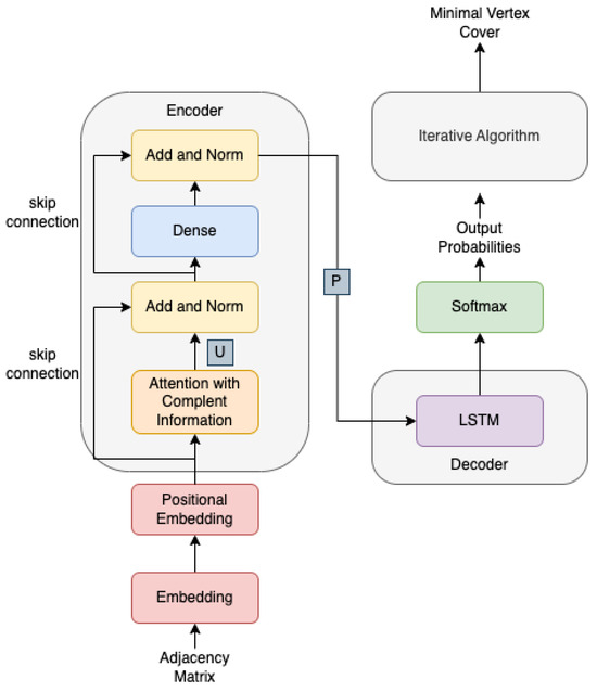
Figure 2.
Schema of the architecture implemented. The input of the architecture is the adjacency matrix of the input graph. The output is the probability that each node belongs to the covering set. The input first passes through an embedding step, which consists of a non-linear transformation of the input plus the positional embedding. This is then passed to the encoder, which is composed of the custom attention layer, which produces a context vector, and a dense layer, which produces a non-linear transformation of such context vector with residual connections. Then, information is given to the decoder, which is composed of an LSTM layer that computes the conditioned probability distribution over nodes, and it is finally normalized by the SoftMax activation layer.
First, this methodology has been designed to cope with one of the main drawbacks of DL-based approaches, i.e., the fact that they build graph representations only considering local information. By exploiting an attention-based approach directly over the adjacency matrix of the graph, which clearly contains both local and global information, the resulting context vector provides an embedded representation of each node that reflects the combinatorial nature of the problem and that considers both node-level and graph-level features.
Considering also the issue according to which for combinatorial optimization over graphs, generic DL-based approaches are adopted without taking into account the characteristics of a specific problem, we also propose to customize this attention mechanism by following the intuition that, when a covering set is built iteratively, a common approach also used by the main heuristics in their initialization algorithms [39,40] is that of adding first nodes with higher degree and with different connections (i.e., connected to different subsets of nodes). Moreover, we considered that complementary to vertex covers are cliques (indeed, given a graph an MVC C in G is an MC in ). Thus, to compute the embedding of nodes, we consider not only the adjacency matrix itself but also the complement of the adjacency matrix as input to the attention mechanism. The complement of the adjacency matrix is used as the key to produce a better representation of the input.
With this customization of the more general attention mechanism, we can encode inductive bias into the DL architecture, thus better capturing the characteristics of the MVC problem. Roughly speaking, this representation is the most important part of the architecture proposed since it embeds the necessary information to let the network compute the conditional probability . Indeed, the context vector U produced is then transformed using a dense layer. We also used residual connections [49] (as is usually done in common DL architectures) among the attention and the dense layer to let information flow through the network, enriching the representation produced. These steps allow the production of a compact representation of the nodes in a latent space that can be processed by the LSTM decoder that converts it to the conditional probability distribution over nodes. The final SoftMax activation layer allows the obtaining of a score associated with each node. This score represents the probability that a node is part of the covering set.
Finally, to grant that the output of the network is a cover, we design a simple algorithm that iteratively adds each node to the covering set based on the score ordering provided by the model. The algorithm is designed following the schema of the initialization algorithm of some common heuristics, thus addressing also the third main drawback of the DL-based approach for combinatorial optimization over graphs by integrating the operation of these common heuristics into the classification procedure.
3.2. Attention with Complement Information
The implementation of the attention mechanism follows the schema represented in Figure 3. To implement Equation (6) as described in [45], we directly use the adjacency matrix A to compute Q and V by first learning H, as the sum of a non-linear transformation of A (which produces an embedded representation of A) and the positional encoding of the input nodes, and then by learning the weights of another linear transformation separately for Q and V. To produce the K matrix, instead, we apply the same procedure to obtained from the complement of the adjacency matrix , where is a matrix with all entries equal to 1. The size of the matrices is kept unchanged so that each row can be referenced to a representation of the node in that position. Equation (10) better describes how matrices Q, K, and V are computed by integrating the complement of the adjacency matrix.
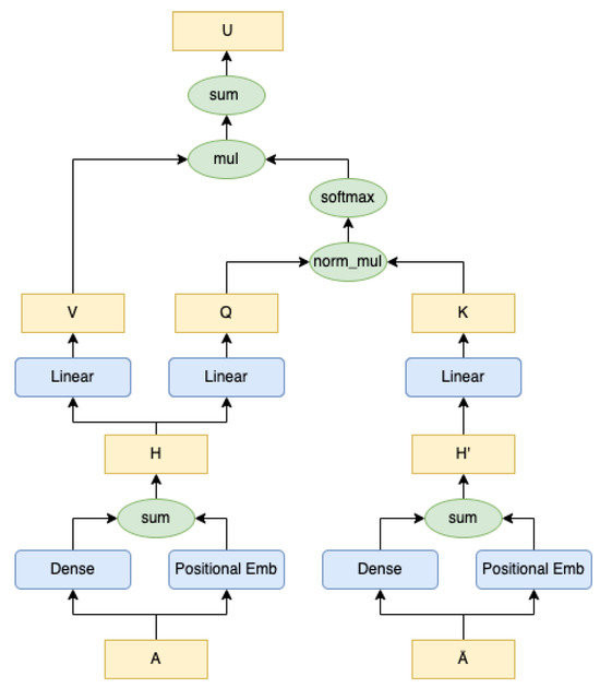
Figure 3.
Schema of the implemented attention mechanism. A is the adjacency matrix of a graph and its complement. The dense layer represents a non-linear transformation performed with the ReLU activation function, the linear layer represents a linear transformation, while the positional embedding is a non-linear transformation of the position of the node in the graph.
In Equation (10), we can see that each transformation (linear or non-linear) has its own matrix of weights and biases, defined by the subscripts, which, thus, is learned separately.
In this way, following the intuition described in Section 3.1, we expect that when computing the alignment score by applying the element-wise product, for each pair of nodes we compute a similarity score between node i and j which is much higher the fewer number of nodes the neighborhood sets of i and j have in common. In this way, the general DL mechanism is customized to reflect the behavior of common heuristics to build the MVC.
Over the alignment score, a SoftMax function is computed to normalize it () and, finally, to produce a weighted representation, they are multiplied by the V matrix as in Equation (6).
The output is a matrix of attention weights for each element of each feature vector (one per node) of the input matrices H and . This matrix is composed of attention coefficients that indicate which node must be assigned more energy for the final computation. Finally, a context vector for each node i is produced by summing all the attention coefficients of each node representation ().
Thus, given a adjacency matrix A, where each row represents a node of the input graph, the matrix of context vectors is a matrix, where each row represent an m-dimensional embedding of the corresponding input node, built considering not only its local features but also its importance with respect to the other nodes in building the MVC.
3.3. LSTM Decoder
The embedding vector produced by the encoder side of the architecture in Figure 2 is then used to produce the final probability distribution as requested by Problem 1. This is carried out by passing as input to the LSTM decoder the sequence of embedding produced . As described in Section 3.3, The LSTM decoder can model the conditional probability distribution as function of the parameters learned during training. During inference, given a sequence the learned parameters are used to select the sequence with the highest probability, i.e., .
To produce the final ordered scores, a SoftMax activation function is applied to the output of the LSTM layer. The final SoftMax activation normalizes the output vector to be an output distribution over the dictionary of inputs.
The entire network is trained to minimize the negative log-likelihood loss function over the log-SoftMax activation function,
where is the target value of the i-th node (i.e., 1 if node i belongs to the covering set, 0 otherwise), and is the computed probability that the i-th node belongs to the covering set.
This loss function is used to ensure that estimated probabilities (assuming that the network is properly trained) actually reflect real ones. Indeed, for each node of the sample graph in input, there is a target value that is either 1 if the corresponding node is a covering node or 0 otherwise. Thus, each predicted class probability is compared to the desired output of 0 or 1. The calculated loss penalizes the probability based on how far it is from the expected value. The penalty is logarithmic, yielding a large score for significant differences close to 1 and a small score for minor differences close to 0.
3.4. Iterative Algorithm
Finally, to grant that the output of the network is a minimal cover, we adapt the ConstructVC algorithm proposed in [40] to use the probability scores produced as outputs by our ACI-based model in place of nodes’ degrees. In this way, we follow the suggestions of common successful heuristics in our DL-based methodology. Indeed, the ConstructVC algorithm is designed to build a minimal vertex cover given a graph iteratively. The modified version of the algorithm we propose is detailed in Algorithm 1 and consists of an extending phase and a shrinking phase. In the extending phase, we start with an empty set C. The algorithm extends C by checking and covering an edge in each iteration: if the considered edge is uncovered, the endpoint with the higher computed probability score is added into C. In the shrinking phase, we first calculate the loss values of vertices in C (where the loss is defined as the number of covered edges that would become uncovered by removing a vertex v from C.); then, we scan the C set and if a vertex has a loss value of 0, it is removed, and loss values of its neighbors are updated accordingly. Since the algorithm proposed follows the structure of the one proposed in [40] and only changes the probability according to which nodes are selected to be part of the final cover C, it can be proved that the vertex set returned by the procedure is a minimal vertex cover.
| Algorithm 1: Build Vertex Cover |
 |
4. Experimental Evaluation
To train the neural model proposed, we create a synthetic dataset composed of randomly generated graphs. The final training dataset is composed of 3000 graphs for training and 600 graphs for validation with a random number of nodes between 5 and 2000. Half of the instances are relatively simple, with a random number of edges between the number of nodes itself and 1.5 times the number of nodes, i.e., low-density instances, and half more complex, with a random number of edges between 5 and 500 times the number of nodes, i.e., high-density instances. Given the number of nodes and the number of edges (iteratively extracted from a uniform distribution as described above), instances are built by choosing a graph uniformly at random from the set of all graphs with the given number of nodes and the given number of edges according to the method described in [50]. For each graph from the simple instances, we compute the cover using a branch-and-bound algorithm [51] to solve exactly the integer linear program formulated in Equation (1), setting as upper bound the initial number of nodes (updated each time to the size of the best solution found), as lower bound the dimension of the current vertex cover plus the dimension of the best vertex cover found for the subproblem considered and starting search from the node with highest degree in the subproblem considered. For each graph from the hard instances, instead, we compute the cover using the FastVC algorithm [40] by setting a cutoff time of 10 s, a maximum number of iterations of 30, and, since FastVC is non-deterministic, for each graph we run the algorithm 5 times and use as ground truth the best solution found. We decided to choose two distinct approaches to build the ground truth first because there is not a publicly available dataset with exact solutions that could fit our case and then because the ILP exact solver can only produce results for very low-density simple instances since the computation time for hard instances is too high for development. Thus, we decided to use simple cases with exact solutions and hard cases with approximate solutions, supposing that if the model can generalize well, simple instances with exact solutions may also let the model learn to produce better solutions for hard cases. We decided to use FastVC since it has been proven in [40] that this is the best-performing heuristic with respect to the other heuristics proposed, like NuMVC [39].
For the same reason, to test the methodology, we build 3 distinct datasets:
- Dataset 1 composed of 22 synthetically generated low-density simple instances and a ground truth computed with the ILP solver used to compare the results of our methodology with respect to exact solutions;
- Dataset 2 composed of 70 synthetically generated high-density hard instances and a ground truth computed with a reference 2-factor approximation algorithm [31];
- Dataset 3 composed of 27 publicly available instances (both low-density and high-density instances) from the DIMACS benchmark graphs [52] and a ground truth computed with the 2-factor approximation algorithm.
4.1. Hyperparameters and Training Results
As far as the common neural network’s hyperparameters are concerned, the network has been trained for 100 epochs, with a batch size and Adam [53] with initial learning rate as optimizer. Both the Input Embedding and the Positional Embedding produce a node representation with an embedding dimension . In the encoder, after the ACI layer, we stacked three dense layers that convert the dimension of the context vector first to (with N maximum number of nodes in the graphs, i.e., 2000), then to and finally produce and embedded vector of size . In the decoder, we used only one LSTM layer that converts the dimension of the embedded vector from to .
We trained the network on a MacBook Pro (2017) with 16 GB of RAM and a 3.1 GHz Intel Core i7 quad-core CPU, and it takes 7 h and 32 m to complete the training.
To ensure that the neural model actually learns how to assign good probability estimates, we measure the network with respect to the classification task for which it is trained. As described in Section 3.3, we train the network minimizing the negative log-likelihood loss function over the log-SoftMax activation function, measuring the performance comparing, for each node of the input graph, the predicted class probability (1, if the corresponding node is a covering node, 0 otherwise) with the desired output. Thus, to be sure that the model properly learns how to assign such estimates, we measure the model using the common metrics for binary classification problems: Accuracy, Precision and Recall, by considering a threshold value for the probability estimates of 0.5 (i.e., if the probability estimate is higher than 0.5, the outcome of the model is 1. Otherwise it is 0). Accuracy measures how often the model correctly predicts the outcome and is measured as the ratio between the number of correct predictions (the sum of true positives and true negatives) and the total number of predictions. Precision measures how often the model correctly predicts the positive class and can be computed as the ratio between the number of correct positive predictions (true positives) and the total number of instances the model predicted as positive (the sum of true and false positives). Recall measures how often the model correctly identifies positive instances from all the actual positive samples in the dataset and can be computed as the ratio between the number of true positives and the number of positive instances (the sum of true positives and false negatives). We measured these three metrics over the two synthetically generated datasets, which, considered together, are composed of a total of 92 graphs with 92,650 nodes. Therefore, these metrics are calculated considering a support of 92,650 samples. Results are shown in Table 1. As we can see, the results show a good percentage for all the metrics (always higher than 82%). This confirms the fact that the probability estimates produced by the neural model actually reflect the real ones. It is important to note, however, that such metrics are not suitable to evaluate the entire methodology with respect to the MVC task for two main reasons: (1) the model is trained to produce probability estimates in a data-driven fashion, thus without constraints that force the final classification to be a minimal cover (this is achieved by the iterative algorithm proposed described in the following); (2) the MVC problem does not have a unique solution, thus even if the model were able to produce probability estimates that result in a minimal cover, if the minimal cover estimated is not exactly the same as the one given as ground truth to be compared against, it would result in poor performance metrics. Therefore, to measure the entire methodology, we rely on a different metric (described in the next paragraph) that takes these aspects into account.

Table 1.
Neural model evaluation metrics (Accuracy, Precision, and Recall) computed over the two synthetically generated datasets composed of a total of 92 graphs. Support represents the total number of samples over which these metrics have been computed, i.e., the total number of nodes.
4.2. Percentage Improvement
To measure the performance of our model for each of the three datasets, since MVC sets may not be unique, we compare the length of the covering sets produced by our ACI-based methodology and by the FastVC heuristic with the length of the covering sets produced by the baseline algorithm used to build the ground truth (ILP solver for the first test set or the 2-factor approximation for the second and third test set), normalizing the distance with respect to the biggest cover obtained by the baseline and the compared method as in the following equation,
where I is the percentage improvement, is the size of the cover produced by the corresponding baseline algorithm, and is the size of the cover produced by the compared methodology.
To compare the results of our methodology with the state-of-the-art solutions FastVC heuristic, we set a cutoff time of 10 s, and a maximum number of iterations of 30, and we ran the algorithm 5 times and used the best solution found.
Table 2 reports the comparison between the results of our methodology and the FastVC heuristic for Dataset 1 and Dataset 2. In the first case, the average improvement represents the average distance of the computed solution from the exact solution. In this case, our methodology can outperform FastVC in better approximating the solution. Indeed, the ACI-based method allows the obtaining of an average distance of −7.21% against the larger distance of −10.61% of FastVC. In the second case, instead, both our methodology and the FastVC heuristic can outperform the 2-factor approximation algorithm, our solution by a percentage of 3.26% and the FastVC heuristic by a percentage of 2.70%. Thus, the proposed methodology can also outperform the FastVC heuristic in this case. These results confirm the fact that the neural model achieves the task of producing probability estimates that actually reflect the combinatorial structure of the problem since, if used together with the iterative algorithm as heuristic to compute a minimal vertex cover, on average, they produce a better approximation than the 2-factor approximation algorithm and than the FastVC heuristic. Another interesting consideration concerns computation time. Clearly, the exact ILP solver is the slowest algorithm, even though instances are relatively small, while the 2-factor approximation is by far the fastest. When it comes to our proposed solution, by analyzing the results, we can see that the computation time is very similar both with low-density instances and with high-density instances. It is important to consider that, on average, 0.19 s are required by the neural model at inference time to produce the node score probability. The rest is used to compute the covering set. The fact that the average time does not increase too much from Dataset 1 with simpler instances to Dataset 2 with harder instances means that our methodology, in general, scales well. As far as FastVC is concerned, the average time considered is the required time to compute the cover, thus the sum of the required times for each run of the algorithm (5 in total for each instance). We can see that, in this case, with low-density instances, the algorithm is very fast. With high-density instances, the required time is almost quadrupled. Of course, the average time is still relatively small; however, this highlights the limits in the scalability of such an algorithm.
Table 2.
Average results of the ACI methods expressed in terms of average percentage improvement I on the first two synthetically generated datasets. A negative value of I indicates that the cardinality of the produced covering set is higher than the cardinality of the set produced by the baseline algorithm and the opposite for a positive value.
The same considerations can be done by analyzing the results over Dataset 3, composed of the publicly available DIMACS benchmark graphs [52]. The results are shown in Table 3. On average (average results are highlighted in the last line), the ACI-based approach produces a percentage improvement of 2.91% with respect to the 2-factor approximation algorithm, while the FastVC heuristic (with the same configuration and number of runs) obtains a percentage improvement of 1.43%. Thus, in this case, even though both algorithms produce a better covering set with respect to the 2-factor approximation algorithm, our proposed solution can also outperform the FastVC heuristic. Even considering execution time, results over Dataset 3 are in line with results over Dataset 1 and 2. Indeed, on average, the ACI-based method requires 0.25 s, while FastVC requires 0.33 s (against the 0.02 s of the 2-factor approximation). It is important to notice that actually, on small instances (e.g., johnson8-2-4), the time required by FastVC is very small compared with the ACI-based method; however, it increases a lot when considering harder instances (e.g., C2000-5, hamming10-2) differently from the ACI-based method where the increase in the computation time is limited. This further confirms the fact that our approach scales better than FastVC with harder instances.
Table 3.
Comparison of the methodologies expressed in terms of size of the minimal cover obtained and time required to compute it on the DIMACS benchmark graphs by each algorithm. Times are expressed in seconds. The last line contains the average results for the time and the average percentage improvement computed according to Equation (12).
It is important to note that our methodology only fits for graphs with no more than 2000 nodes. This is not a strong limit for many real-world applications like network design, sensor network, resource allocation, or text tasks [2,4,5]. To test the methodology with larger graphs, it would be necessary to retrain the neural model by modifying the maximum size of the graph to be expected as input. However, we did not explore this aspect of the research further.
4.3. Nodes Representation
Another important aspect of our approach concerns the capability of the network, particularly of the ACI-based method, to produce a good representation of the nodes with respect to the optimization target defined by the MVC problem. To understand whether the network can perform a proper mapping of the embedded input nodes into a d-dimensional space, we plot some points considering the representation of the nodes as obtained from the output of the ACI layer of the network, namely the context vector U. Since the network has been trained to produce an encoding embedding in a 32-dimensional space, we only visualize a scatterplot of the nodes by taking two of the 32 components at a time. We only visualize the results with respect to the first four components since the behavior is similar for the others as well. In Figure 4, we can see the representation of the nodes of a graph with 25 nodes and 50 edges. The orange points are the points associated with covering nodes according to the exact solution, while the blue ones are those that do not correspond to covering nodes. In general, we can see that the network is able to map the points in a space where covering nodes and non-covering nodes belong to different regions (almost linearly separable) and with a clear ordering.
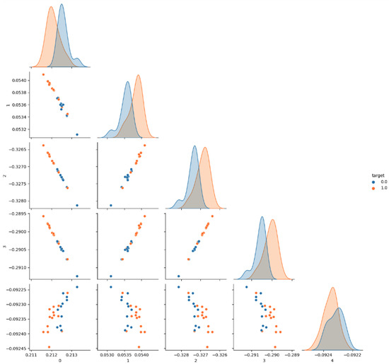
Figure 4.
Example of nodes representations of a graph as produced by the ACI layer with respect to the first four components taken in pairs. In blue, we can see points that do not belong to the covering set, while in orange, we can see the points that belong to the covering set according to the results of the exact ILP solver. On the diagonal, we can see the distribution of such points according to their class (0 or 1). We can see that, despite some overlapping, orange and blue points present different distributions.
This representation is built considering node features so that similar nodes are closer in this representation space. Figure 5 shows an example of this. In the picture, we can see the input graph (with 10 nodes and 15 edges), with covering nodes represented in red and non-covering nodes represented in blue. Together with the graph, the representation of the nodes (with respect to 2 random dimensions of the context vector) is visualized by tagging each point with the corresponding index of the node and color. From the picture, we can see that, as an example, nodes 1 and 2 are close to each other. Indeed, they both have a degree equal to 5, and they are both connected to nodes 4, 9, and 0. Therefore, they are very similar. Analogous reasoning can be done for node 3, which is very similar to 2 and 1, and for nodes 8 and 5, which are very similar to each other. Moreover, if, on the one hand, this representation is interesting and reasonable, the final probability estimates which are built considering this representation, do not perfectly reflect this representation since, as an example, considering the graph in Figure 5, nodes 9 and 8 have a higher probability score with respect to node 0 (the final order with respect to the probability score is: 1, 3, 2, 9, 8, 0, 6, 4, 5, 7). This means that the decoder component of the network also plays a very important role in producing the final result. Moreover, the order produced is quite far from the order that we would obtain, considering only the degree. Thus, it is not surprising that the result obtained using these probability estimates in the ConstructVC algorithm is different from the result obtained using the degree (as for FastVC).
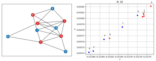
Figure 5.
Example of a graph with 10 nodes and 15 edges and its representation considering 2 random dimensions of the context vector. Covering nodes are shown in red, while non-covering nodes are in blue. This representation shows how similar nodes are closer in the representation space.
The fact that our methodology outperforms the FastVC heuristic, instead, makes clear that the implemented approach manages to reflect the combinatorial structure of MVC problems and that the probability estimates produced by our neural model are a better driver for building the MVC with respect to node degree. This is due to the fact that, on the one hand, we build node representations considering both local and global information by applying the attention mechanism directly to the adjacency matrix, and on the other hand, it is due to the fact that the customization proposed, which reflects common heuristics procedures to build the MVC, actually induces a good bias to represents nodes with respect to the specific problem considered. Specifically, these results show that the proposed customization of the attention mechanism manages the task of assigning a higher score to nodes that should be part of the MVC set, making the iterative algorithm proposed a good approach to build the final covering set.
5. Conclusions and Future Works
In this paper, we have presented an approach to solving MVC problems over graphs, mainly using attention. In designing the approach, we tried to tackle three main issues related to the DL-based approach for combinatorial optimization over graphs: (1) build a suitable graph representation at node level using both global and local information; (2) customize a common DL approach to reflect the combinatorial structure of the MVC problem; (3) integrate the DL methodology with state-of-the-art heuristics to take advantage of them.
To cope with issues 1 and 2, we proposed a methodology that makes use of what we called Attention with Complement Information, i.e., a mechanism of attention which first of all is applied over graphs adjacency matrix to use both local and global information, and then that takes as input not only the matrix itself but also the complement of the matrix, following the intuition, commonly implied also by many state-of-the-art heuristics, that in order to identify candidate nodes to a covering set, it could be useful to know their interaction with other nodes and that the complement of such interaction may provide a better scoring when two nodes have similar interactions. We then use the output of such attention mechanism, properly transformed, as input to an LSTM-based decoder network followed by a SoftMax activation layer to produce the final probability distribution.
We showed that our methodology can outperform not only a common 2-factor approximation algorithm for MVC but also a widely used state-of-the-art heuristic known as FastVC both on low-density graphs and on higher-density graphs. Moreover, if our approach is relatively slower with low-density graphs with respect to both the 2-factor approximation algorithm and the FastVC heuristic, it scales much better than FastVC on higher-density graphs. This represents a great advantage, also meaning that for MVC tasks on graphs of comparable size to the ones used to train our neural model, our methodology should be preferred to other state-of-the-art approaches.
Finally, we also proved that our attention mechanism with complement information manages to draw a proper representation of the nodes according to the combinatorial nature of the MVC problem. This is extremely important since it demonstrates that our work manages to address the three main issues of the DL-based approach for combinatorial optimization over graphs. As far as we know, this makes our proposal one of the firsts to address these main challenges successfully. Nonetheless, another advantage of our methodology is that we provide a new validated method to build node embeddings in a meaningful way. The embeddings produced, indeed, could be used and tested also for different task-related MVC problems. In this research, we have explained that there is a strong similarity between the iterative algorithm proposed to build the final solution of our method and the iterative algorithm used by FastVC to initialize its solution. However, in FastVC, after initializing the solution, the authors propose to refine the solution by changing the nodes in the covering set according to a cost-effective heuristic called Best from Multiple Selections (BMS). Thus, a possible future direction of this work could be that of understanding how, by applying the BMS heuristic, we could improve the results and in which time.
We consider this work as a step towards a new family of solvers for NP-hard problems that leverages and customize DL properly, and, in particular, we will try to extend the results of such work also on the less explored context of temporal networks, where many combinatorial NP-hard problems, like the minimum timeline cover [27,54], do not have an approximate solution.
Author Contributions
Conceptualization, G.L., R.D., S.M. and I.Z.; methodology, G.L. and I.Z.; software, G.L.; validation, R.D., S.M. and I.Z.; formal analysis, G.L. and I.Z.; investigation, G.L.; resources, G.L., R.D. and I.Z.; data curation, G.L. and R.D.; writing—original draft preparation, G.L.; writing—review and editing, R.D., S.M. and I.Z.; supervision, S.M. and I.Z.; project administration, S.M. and I.Z. All authors have read and agreed to the published version of the manuscript.
Funding
This research received no external funding.
Data Availability Statement
Data are contained within this article.
Conflicts of Interest
The authors declare no conflict of interest.
References
- Angel, D. A graph theoretical approach for node covering in tree based architectures and its application to bioinformatics. Netw. Model. Anal. Health Inf. Bioinform. 2019, 8, 12. [Google Scholar]
- Yigit, Y.; Akram, V.K.; Dagdeviren, O. Breadth-first search tree integrated vertex cover algorithms for link monitoring and routing in wireless sensor networks. Comput. Netw. 2021, 194, 108144. [Google Scholar] [CrossRef]
- Cheng, T.M.K.; Lu, Y.E.; Vendruscolo, M.; Lio’, P.; Blundell, T.L. Prediction by graph theoretic measures of structural effects in proteins arising from non-synonymous single nucleotide polymorphisms. Netw. Model. Anal. Health Inf. Bioinform. 2019, 8, 12. [Google Scholar] [CrossRef]
- Gupta, A.; Kaur, M. Text summarisation using Laplacian centrality-based minimum vertex cover. J. Inf. Knowl. Manag. 2019, 18, 1950050. [Google Scholar] [CrossRef]
- Probierz, B.; Hrabia, A.; Kozak, J. A New Method for Graph-Based Representation of Text in Natural Language Processing. Electronics 2023, 12, 2846. [Google Scholar] [CrossRef]
- Bhattacharya, S.; Henzinger, M.; Nanongkai, D. Fully dynamic approximate maximum matching and minimum vertex cover in O(log3 n) worst case update time. In Proceedings of the 2017 Annual ACM-SIAM Symposium on Discrete Algorithms, Barcelona, Spain, 16–19 January 2017; pp. 470–489. [Google Scholar]
- Ghaffari, M.; Jin, C.; Nilis, D. A massively parallel algorithm for minimum weight vertex cover. In Proceedings of the 32nd ACM Symposium on Parallelism in Algorithms and Architectures, Virtual Event, 15–17 July 2020; pp. 259–268. [Google Scholar]
- Onak, K.; Ron, D.; Rosen, M.; Rubinfeld, R. A near-optimal sublinear-time algorithm for approximating the minimum vertex cover size. In Proceedings of the 23rd Annual ACM-SIAM Symposium on Discrete Algorithms, Kyoto, Japan, 17–19 January 2012; pp. 1123–1131. [Google Scholar]
- Dondi, R.; Mauri, G.; Zoppis, I. Clique Editing to Support Case versus Control Discrimination. In Proceedings of the 8th KES International Conference on Intelligent Decision Technologies—Part I, Tenerife, Spain, 15–17 June 2016; pp. 27–36. [Google Scholar]
- Reba, K.; Guid, M.; Rozman, K.; Janežič, D.; Konc, J. Exact Maximum Clique Algorithm for Different Graph Types Using Machine Learning. Mathematics 2022, 10, 97. [Google Scholar] [CrossRef]
- Pop, P.C.; Cosma, O.; Sabo, C.; Sitar, C.P. A comprehensive survey on the generalized traveling salesman problem. Eur. J. Oper. Res. 2024, 314, 819–835. [Google Scholar] [CrossRef]
- Yakıcı, E. A heuristic approach for solving a rich min-max vehicle routing problem with mixed fleet and mixed demand. Comput. Ind. Eng. 2017, 109, 288–294. [Google Scholar] [CrossRef]
- Garey, M.R.; Johnson, D.S. Computers and Intractability: A Guide to the Theory of NP-Completeness; W. H. Freeman and Co., Ltd.: San Francisco, CA, USA, 1979. [Google Scholar]
- Dean, W. Computational Complexity Theory; Stanford University: Stanford, CA, USA, 2021. [Google Scholar]
- Gonzales, T.F. Handbook of Approximation Algorithms and Metaheuristics, 2nd ed.; Chapman and Hall/CRC: London, UK, 2020. [Google Scholar]
- Oriol, V.; Meire, F.; Navdeep, J. Pointer networks. In Proceedings of the 28th International Conference on Neural Information Processing Systems—Volume 2, San Francisco, CA, USA, 7–12 December 2015; pp. 2692–2700. [Google Scholar]
- Graves, A.; Wayne, G.; Reynolds, M.; Harley, T.; Danihelka, I.; GrabskaBarwinska, A.; Colmenarejo, S.G.; Grefenstette, E.; Ramalho, T.; Agapiou, J. Hybrid computing using a neural network with dynamic external memory. Nature 2016, 538, 471–476. [Google Scholar] [CrossRef]
- Dai, H.; Khalil, E.B.; Zhang, Y.; Dilkina, B.; Song, L. Learning combinatorial optimization algorithms over graphs. In Proceedings of the 31st International Conference on Neural Information Processing Systems, Long Beach, CA, USA, 4–9 December 2017; pp. 6351–6361. [Google Scholar]
- Silver, D.; Huang, A.; Maddison, C.J.; Guez, A.; Sifre, L.; Van den Driessche, G.; Schrittwieser, J.; Antonoglou, I.; Panneershelvam, V. Mastering the game of Go with deep neural networks and tree search. Nature 2016, 529, 484–489. [Google Scholar] [CrossRef] [PubMed]
- Bello, I.; Pham, H.; Le, Q.V.; Norouzi, M.; Bengio, S. Neural combinatorial optimization with reinforcement learning. In Proceedings of the 5th International Conference on Learning Representation, Toulon, France, 24–26 April 2017. [Google Scholar]
- Abu-Khzam, F.N.; Abd El-Wahab, M.M.; Haidous, M. Learning from obstructions: An effective deep learning approach for minimum vertex cover. Ann. Math. Artif. Intell. 2022, 1–12. [Google Scholar] [CrossRef]
- Gianinazzi, L.; Fries, M.; Dryden, N.; Ben-Nun, T.; Besta, M.; Hoefler, T. Learning Combinatorial Node Labeling Algorithms. arXiv 2022, arXiv:2106.03594. [Google Scholar]
- Li, Z.; Chen, Q.; Koltun, V. Combinatorial optimization with graph convolutional networks and guided tree search. In Proceedings of the 32nd International Conference on Neural Information Processing Systems, Montreal, QC, Canada, 3–8 December 2018; pp. 537–546. [Google Scholar]
- Langedal, K.; Langguth, J.; Manne, F.; Schroeder, D.T. Efficient minimum weight vertex cover heuristics using graph neural networks. In Proceedings of the 20th International Symposium on Experimental Algorithms, Heidelberg, Germany, 25–27 July 2022; pp. 1–17. [Google Scholar]
- Vesselinova, N.; Steinert, R.; Perez-Ramirez, D.F.; Boman, M. Learning Combinatorial Optimization on Graphs: A Survey with Applications to Networking. IEEE Access 2020, 8, 120388–120416. [Google Scholar] [CrossRef]
- Peng, Y.; Choi, B.; Xu, J. Graph Learning for Combinatorial Optimization: A Survey of State-of-the-Art. Data Sci. Eng. 2021, 6, 119–141. [Google Scholar] [CrossRef]
- Rozenshtein, P.; Tatti, N.; Gionis, A. The network-untangling problem: From interactions to activity timelines. Data Min. Knowl. Disc. 2021, 35, 213–247. [Google Scholar] [CrossRef]
- Dinur, I.; Khot, S.; Kindler, G.; Minzer, D. On independent sets, 2-to-2 games, and Grassmann graphs. In Proceedings of the 49th Annual ACM SIGACT Symposium on Theory of Computing, Montreal, QC, Canada, 19–23 June 2017; pp. 576–589. [Google Scholar]
- Khot, S.; Regev, O. Vertex cover might be hard to approximate to within 2-epsilon. J. Comput. Syst. Sci. 2008, 74, 335–349. [Google Scholar] [CrossRef]
- Karakostas, G. A better approximation ratio for the vertex cover problem. ACM Trans. Algorithms 2009, 5, 1–8. [Google Scholar] [CrossRef]
- Bar-Yehuda, R.; Even, S. A local-ratio theorem for approximating the weighted vertex cover problem. Ann. Discret. Math. 2018, 25, 27–46. [Google Scholar]
- NetworkX Documentation, Min_Weighted_Vertex_Cover. Available online: https://networkx.org/documentation/stable/reference/algorithms/generated/networkx.algorithms.approximation.vertex_cover.min_weighted_vertex_cover.html (accessed on 2 February 2023).
- Singh, M. Integrality gap of the vertex cover linear programming relaxation. Oper. Res. Lett. 2019, 47, 288–290. [Google Scholar] [CrossRef]
- Tomita, E.; Kameda, T. An efficient branch-and-bound algorithm for finding a maximum clique with computational experiments. J. Glob. Optim. 2009, 44, 311. [Google Scholar] [CrossRef][Green Version]
- Li, C.M.; Quan, Z. Combining graph structure exploitation and propositional reasoning for the maximum clique problem. In Proceedings of the 22nd IEEE International Conference on Tools with Artificial Intelligence, Arras, France, 27–29 October 2010; pp. 344–351. [Google Scholar]
- Li, C.M.; Quan, Z. An efficient branch-and-bound algorithm based on maxsat for the maximum clique problem. In Proceedings of the 24th AAAI Conference on Artificial Intelligence, Atlanta, GA, USA, 11–15 July 2010; pp. 128–133. [Google Scholar]
- Hespe, D.; Lamm, S.; Schulz, C.; Strash, D. WeGotYouCovered: The winning solver from the pace 2019 challenge, vertex cover track. In Proceedings of the 2020 SIAM Workshop on Combinatorial Scientific Computing, Seattle, WA, USA, 11–13 February 2020; pp. 1–11. [Google Scholar]
- Chen, J.; Kanj, I.A.; Xia, G. Improved upper bounds for vertex cover. Theor. Comput. Sci. 2020, 411, 3736–3756. [Google Scholar] [CrossRef]
- Cai, S.; Su, K.; Luo, C.; Sattar, A. NuMVC: An Efficient Local Search Algorithm for Minimum Vertex Cover. J. Artif. Intell. Res. 2023, 46, 687–716. [Google Scholar] [CrossRef]
- Cai, S. Balance between Complexity and Quality: Local Search for Minimum Vertex Cover in Massive Graphs. In Proceedings of the 24th International Joint Conference on Artificial Intelligence, Buenos Aires, Argentina, 25–31 July 2015; pp. 747–753. [Google Scholar]
- Cai, S.; Li, Y.; Hou, W.; Wang, H. Towards faster local search for minimum weight vertex cover on massive graphs. Inf. Sci. 2019, 471, 64–79. [Google Scholar] [CrossRef]
- Cai, S.; Hou, W.; Lin, J.; Li, Y. Improving Local Search for Minimum Weight Vertex Cover by Dynamic Strategies. In Proceedings of the 27th International Joint Conference on Artificial Intelligence, Stockholm, Sweden, 13–19 July 2018; pp. 1412–1418. [Google Scholar]
- Bahdanau, D.; Cho, K.; Bengio, Y. Neural Machine Translation by Jointly Learning to Align and Translate. In Proceedings of the 3rd International Conference on Learning Representations, San Diego, CA, USA, 7–9 May 2015. [Google Scholar]
- Dubey, S.R.; Singh, S.K.; Chaudhuri, B.B. Activation functions in deep learning: A comprehensive survey and benchmark. Neurocomputing 2022, 503, 92–108. [Google Scholar] [CrossRef]
- Vaswani, A.; Shazeer, N.; Parmar, N.; Uszkoreit, J.; Jones, L.; Gomez, A.; Kaiser, L.; Polosukhin, I. Attention is all you need. In Proceedings of the 31st Conference on Neural Information Processing Systems, Long Beach, CA, USA, 4–9 December 2017. [Google Scholar]
- Elman, J.L. Finding structure in time. Cogn. Sci. 1990, 14, 179–211. [Google Scholar] [CrossRef]
- Hochreiter, S.; Schmidhuber, J. Long Short-term Memory. Neural Comput. 1997, 9, 1735–1780. [Google Scholar] [CrossRef]
- Akbik, A.; Blythe, D.; Vollgraf, R. Contextual String Embeddings for Sequence Labeling. In Proceedings of the 27th International Conference on Computational Linguistics, Santa Fe, NM, USA, 20–26 August 2018; pp. 1638–1649. [Google Scholar]
- He, K.; Zhang, X.; Ren, S.; Sun, J. Deep residual learning for image recognition. In Proceedings of the IEEE Conference on Computer Vision and Pattern Recognition, Las Vegas, NV, USA, 27– 30 June 2016; pp. 770–778. [Google Scholar]
- NetworkX Documentation: Gnm_Random_Graph. Available online: https://networkx.org/documentation/stable/reference/generated/networkx.generators.random_graphs.gnm_random_graph.html (accessed on 18 January 2024).
- Morrison, D.R.; Jacobson, S.H.; Sauppe, J.J.; Sewell, E.C. Branch-and-bound algorithms: A survey of recent advances in searching, branching, and pruning. Discret. Optim. 2016, 19, 79–102. [Google Scholar] [CrossRef]
- Rossi, R.A.; Nesreen, A.K. The Network Data Repository with Interactive Graph Analytics and Visualization. In Proceedings of the 29h AAAI Conference on Artificial Intelligence, Austin, TX, USA, 25–29 January 2015; pp. 4292–4293. [Google Scholar]
- Kingma, D.P.; Ba, A.J. A method for stochastic optimization. In Proceedings of the 3rd International Conference on Learning Representations, San Diego, CA, USA, 7–9 May 2015. [Google Scholar]
- Dondi, R. Untangling temporal graphs of bounded degree. Theor. Comput. Sci. 2023, 969, 114040. [Google Scholar] [CrossRef]


Disclaimer/Publisher’s Note: The statements, opinions and data contained in all publications are solely those of the individual author(s) and contributor(s) and not of MDPI and/or the editor(s). MDPI and/or the editor(s) disclaim responsibility for any injury to people or property resulting from any ideas, methods, instructions or products referred to in the content. |
© 2024 by the authors. Licensee MDPI, Basel, Switzerland. This article is an open access article distributed under the terms and conditions of the Creative Commons Attribution (CC BY) license (https://creativecommons.org/licenses/by/4.0/).