Abstract
In this study, we created an accurate model for a homogenous smart structure. After modeling multiplicative uncertainty, an ideal robust controller was designed using μ-synthesis and a reduced-order H-infinity Feedback Optimal Output (Hifoo) controller, leading to the creation of an improved uncertain plant. A powerful controller was built using a larger plant that included the nominal model and corresponding uncertainty. The designed controllers demonstrated robust and nominal performance when handling agitated plants. A comparison of the results was conducted. As an example of a general smart structure, the vibration of a collocated piezoelectric actuator and sensor was controlled using two different approaches with strong controller designs. This study presents a comprehensive simulation of the oscillation suppression problem for smart beams. They provide an analytical demonstration of how uncertainty is introduced into the model. The desired outcomes were achieved by utilizing Simulink and MATLAB (v. 8.0) programming tools.
1. Introduction
Many researchers [1,2,3] have investigated smart structures and the suppression of oscillations caused by external disturbances. The field of smart structures has significantly developed in recent years [4,5,6,7]. Damping oscillations require the use of smart materials and the application of controls [8,9,10,11,12]. Advanced verification techniques must be used to account for modeling uncertainties and imperfections. Such techniques can include μ-analysis, μ-synthesis, and robust control. In this study, we used the above types of controls and applied them to smart piezoelectric structures. H-infinity feedback optimal output (Hifoo) control in smart piezoelectric structures involves designing controllers that minimize the impact of disturbances and uncertainties on the output performance of the system. This is particularly important in applications where precise control of the deformation or vibration of the structure is required. Modeling with Hifoo assumes infinite control knowledge. Hinfinite control is a common approach for vibration control [13,14,15,16]. Hifoo is related to H-infinity control, which aims to minimize the effects of disturbances and uncertainties in a system. Hifoo is specifically focused on finding optimal controllers to achieve the best possible output performance. The key benefits of applying μ-analysis control to smart piezoelectric structures include improved robustness against external disturbances, increased stability, and enhanced tracking of the desired responses. These controllers are designed to optimize the trade-off between performance and robustness, making them suitable for applications in which maintaining a specific structural response is critical.
A combination of μ-analysis and Hifoo [4,5,6,17] reduced control theory was utilized to study the design of piezoelectric active control for both normal and damaged smart buildings. The outcomes validated the efficacy of the proposed model and procedures and the control behavior of the beam aligned with expectations. Following a thorough study, we assessed the robustness and performance of the system.
By adding uncertainty, we were able to maintain the framework within specified uncertainty bounds [7,18,19,20]. In a research paper that explored the benefits of robust control in smart structures, refs. [19,20,21,22,23,24] underscored the utilization of Hifoo control [4,5,6,17] in both the state space and frequency domains. The advantages of this work are as follows: the introduction of control for oscillation suppression and the modeling of intelligent structures bring about alterations in both the frequency and time-space domains, as well as the inclusion of uncertainties in the mathematical model of the construction, and an introduction to μ-synthesis and reduced-order control in intelligent structures [25,26]. The development of control strategies for intelligent piezoelectric structures involves several challenging issues. Researchers have investigated the application of piezoelectric materials in systems with distributed parameters with the aim of facilitating efficient and cost-effective active control. Dynamic systems can be actively controlled using distributed sensors and actuators composed of adaptable piezoelectric materials. The main considerations that structural control engineers need to keep in mind while creating reliable control techniques for assessing resilience, optimal placement, and structural modeling in the face of uncertainty are covered in this essay [27,28,29,30]. Because the controller provided is of order 56, sophisticated control techniques may be applied to simpler models, and we use the optimization method Hifoo to reduce the order of the controller. All simulations were completed using sophisticated programming methods in the Matlab software platform (v. 8.0, Mathworks, Natick, MA, USA). A crucial engineering problem is the vibration suppression that occurs under dynamic and unexpected loads. Vibrations are significant in engineering systems because of their association with material deterioration, which can result in major and component failures.
The μ-synthesis process aims to optimize the controller to meet these specifications while accounting for uncertainties. Applying μ-synthesis in the design of controllers for smart structures helps to address the challenges associated with real-world variability and disturbances, making the structures more reliable and adaptive to changing conditions. Moreover, we specify the desired performance criteria for a smart structure, such as concerning response time and vibration suppression. This approach is particularly relevant in applications such as adaptive building structures, aerospace systems, and other fields where the performance of structures is critical.
2. Methodology
μ-Analysis and μ-Synthesis
μ-Analysis is a method used to analyze the robustness of a control system. It quantifies the extent to which the performance of the system can be degraded in the presence of uncertainties or variations in the plant (the system being controlled). This involves considering uncertainties in the system parameters, dynamics, and disturbances. These uncertainties are typically represented by transfer functions of varying magnitudes and phases. μ-Synthesis is an extension of μ-analysis, which incorporates a synthesis or design component. This is a systematic method for designing controllers that can handle identified uncertainties and variations, ensuring robust stability and performance. The μ-synthesis approach involves finding a controller that minimizes the μ-value (uncertainty measure) while satisfying certain performance and stability specifications.
Every approach to the analysis problem discussed includes implements to assess each controller’s performance and facilitate comparisons between controllers. However, a controller that attains a particular performance level in relation to the structured single value μ can be synthesized. The (D, G-K) iteration procedure was used to perform this synthesis [29,31,32]. During this procedure, the task of locating a μ-optimal controller K satisfying μ(Fu(F(jω), K(jω)) ≤ β for all ω has been altered for the challenge of determining the transfer function matrices D(ω) ∈ D and G(ω) ∈ G. Thus,
Unfortunately, this approach does not ensure the discovery of local maxima. Nevertheless, when dealing with intricate perturbations, there is an alternative method called D-K iteration (also executable in MATLAB) [29,33]. This technique integrates μ-synthesis and μ-analysis and frequently provides satisfactory results. It begins with an initial estimation of μ, as stated in connection with the scaled singular value:
The vision is centered on identifying the controller that minimizes the peak value of its upper bound across different frequencies. In other words, the K-Steps in μ-Synthesis are:
Uncertainty Modeling: Identify and model uncertainties in the system. This may include parametric uncertainties, unmodelled dynamics, and external disturbances.
μ-Analysis: Perform μ-analysis to quantify the robustness of the system in the presence of uncertainties. This step helps to identify the critical frequencies and magnitudes wherein robustness is the most challenging.
Robustness: μ-synthesis provides a systematic approach for designing controllers that are robust against uncertainties, ensuring stable and satisfactory performance over a range of operating conditions. The resulting controllers often have a structured form, which makes them more interpretable and easier to implement.
By alternately minimizing the with respect to either K or D (while keeping the other constant) [27,29]:
In the K-step, synthesize an H∞ controller for the scaled problem, minimizing ∥〖DN(Κ)D〗−1 ∥∞ with a fixed D(s).
In the D-step, we determine D(jω) at each frequency to minimize ((jω)) with the fixed transfer function N.
The magnitude of each element of D(jω) is adjusted to fit a stable and minimum-phase transfer function D(s) and then returns to the first step.
3. Results
3.1. Application in Smart Structures
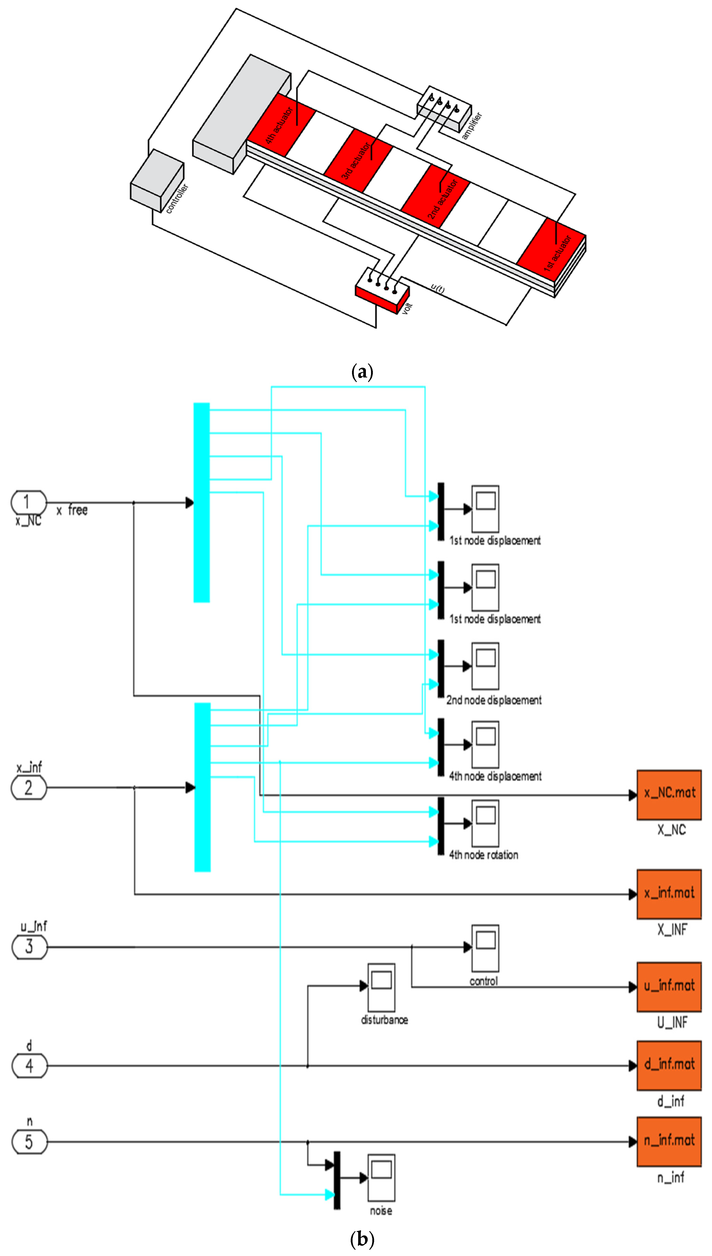
This section examines an eight-element cantilever smart structure (Figure 1a), in which four pairs of piezoelectric patches at the top and bottom surfaces of each beam element are symmetrically bonded. The measurements of several sections of this building are shown below, and Table 1 lists the beam specifications.

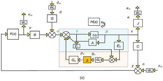
Figure 1.
(a) Modeling of intelligent structure. (b) The block diagram in Matlab Simulink for the smart beam disturbance rejection. (c) The robust control design diagram of μ-synthesis.

Table 1.
Parameters of the smart structure.
Smart structures often involve the integration of sensors, actuators, and control systems to adapt to changing environmental conditions. The dynamical equation for smart structures can be complex and depend on the specific configuration and components used. In the next section, we examine the performance of an eight-element cantilever smart structure featuring four pairs of piezoelectric patches symmetrically affixed to both the top and bottom surfaces of each beam element. The section that follows lists the dimensions of each part of the intelligent structure. The following equations clarify the dynamic characterization of the system:
These equations capture the essence of how smart structures incorporate active and robust controls to adapt to dynamic loads or changing conditions. The challenge lies in designing effective control algorithms and systems that respond optimally to the state of the structure and external forces.
Where K represents the global stiffness matrix, fm is the global external loading vector, and fe is the global control force vector produced by the electromechanical coupling effect, which is often determined by a feedback control system that uses sensor information to adjust the behavior of the structure in real-time. The overall goal is to optimize the performance or response of the structure under varying conditions. M represents the global mass matrix; D represents the viscous damping matrix. The mass Μ and stiffness Κ matrices were derived by assembling the local mass and stiffness matrices. The analysis was performed using Euler Bernoulli’s theory, and we had two degrees of freedom at each node: vertical displacement and rotation. Damping D is a small percentage (0.0005) of the mass and stiffness matrices. The rotations ψi and vertical displacement wi constitute independent variable q(t), i.e.,
where n denotes the number of finite elements used in the analysis. Vectors w and fm were positive upward.
To convert to a state-space control representation, allow (in the usual manner):
In addition, fe(t) can be defined as Bu(t) by expressing it as , where (of size 2n × n) stands for the piezoelectric force for a unit established on the associated actuator [34,35,36], and u represents the voltages on the actuators [34,35,36]. Finally, d(t) = fm(t) denotes the disturbance vector. Then,
In this form, d is a 2n × 1 vector (where n is the number of nodes), and u is, at most, an n × 1 vector (but it may be smaller). The units used were Newton (N), seconds (s), radians (rad), and meters (m). With a more detailed investigation of the stability in the frequency domain, our approach preserves the stability in the time domain [27].
y(t) = [x1(t) x3(t) … xn−1(t)]T = Cx(t)
This state-space representation captures the first-order dynamics of the smart structure, where the state vector x(t) includes both displacement and velocity. Let us now use the following approach to the uncertainty in the M and K matrices:
Furthermore, since D = 0.0005 (K + M), a suitable form for D is as follows:
However, given that, in general:
D = αK + βM
The structural damping matrix D can be examined as a linear combination of mass and stiffness (Rayleigh damping). In this context, the values for α and β were determined based on the first and second normal modes of vibration, with both α and β set at 0.0005. D can be expressed in a manner similar to K and M, as follows:
D = D0 (I + dpI2n×2nδD)
In the pertinent matrices, we incorporate uncertainty in the form of proportional deviation. Given the precision with which the length can be measured, this formulation of uncertainty aligns well with our context. It is more probable that uncertainty originates from factors other than the primary matrices. In this context, we assume that
Hence, mp and kp are used to scale the value of the proportion, and the nominal values are represented by the zero subscript.
(It is urged that, for matrix An×m, the norm is determined via ║A║∞ = .)
Taking these specifications into consideration, Equation (4) changes to,
where:
Equation (7), when expressed in state-space form, generates
In this method, we considered the uncertainty of the original matrices as an additional uncertainty parameter. Incorporating uncertainty into the equation for a smart structure involves modeling the uncertainty in the parameters of the system. In our paper, we introduce uncertainty in the matrices of smart structures and robust control theory, such as μ-analysis and Hifoo control.
3.2. Robust Synthesis: μ-Controller
μ-Analysis, also known as mu-analysis, is a technique commonly used in control system design to analyze and address uncertainties in dynamic systems. This is particularly useful for understanding how uncertainties affect the robustness and stability of control systems. We applied μ-analysis to our smart structures. In μ-analysis, the goal is to assess the system performance in the presence of uncertainty by defining a performance metric denoted by μ. The uncertainty is bounded by identical constraints with a constant mp and kp [29,37,38,39]. All the results were obtained using MATLAB Simulink (Figure 1b); moreover, in all simulations, noise as a percentage ± 2% of the disturbance was obtained. The results are for the displacements and rotations of the smart beam nodes. In Figure 1b, a block diagram for smart beam disturbance rejection in MATLAB Simulink is presented. In the first result, a concentrated load of 10 N was applied to the edge of the support. Subsequently, a sinusoidal load with an oscillation part of 10 N and a period of 1 s was applied. Therefore, for the first mechanical load, we have 10 N at the edge of the cantilever, while, for the second mechanical load, we have a sinusoidal load in the 10 N range with a period of 1 s.
This study uses advanced control techniques and finite element modeling with applications to smart materials. For this reason, because modeling requires many computational requirements, experimental results will be the subject of future research.
mp = 0, kp = ±0.9: This relates to a deviation of approximately 90% from the nominal value of stiffness matrix K (Equations (9) and (10)).
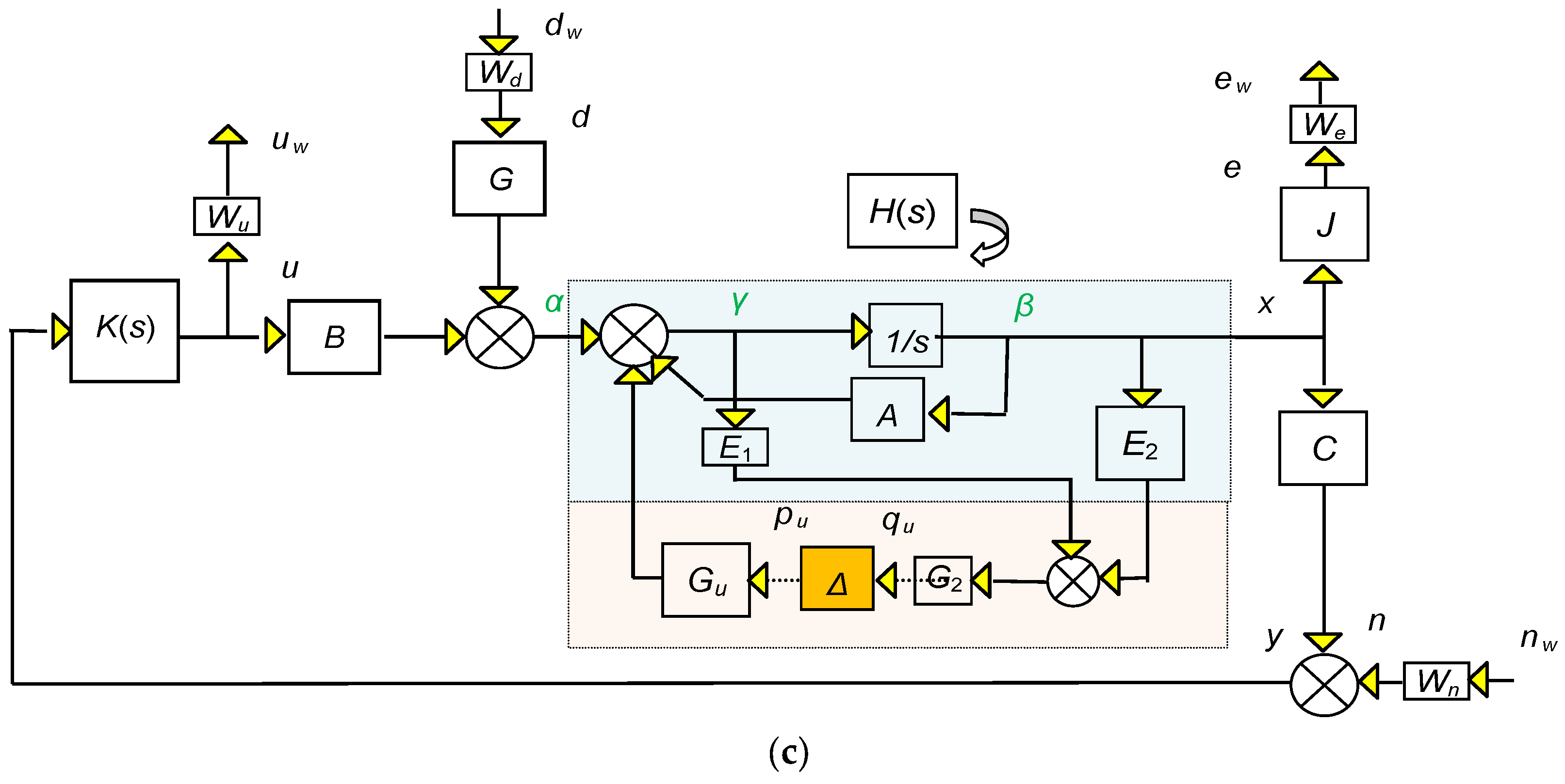
As previously stated, the following commands were required to conduct this process in the MATLAB software platform (Mathworks, Natick, MA, USA) and are presented in Appendix A of the manuscript. This command generates a robust controller on the order of 56. This is a large value because of the operation of this algorithm. Despite being mentioned in the literature, this point has not been given enough emphasis, which is undoubtedly an oversight. To the best of our knowledge, lowering the order cannot be performed quickly without employing a laborious manual process. Figure 1c shows the μ-synthesis robust control design framework.
The white matrix for noise, control, error, and disturbance is for the control (u):
For error e:
For disturbances d:
For noise n:
In the μ-synthesis robust control design diagram, the primary focus is on enhancing the robustness of the system to uncertainties. The process involves evaluating the performance metric μ by analyzing the closed-loop transfer function, considering both the system transfer function T(s) and uncertainty transfer function Δ(s). The goal is to optimize the controller parameters to maximize μ, ensuring improved stability and performance in the presence of uncertainties.
The first mechanical load in each of the simulations that came after the disturbance was 10 N at the free end; K(s) is the controller, Δ is the uncertainty plan (Equation (12)), B (Figure 1a) is the smart structure, and x and y are from Equations (7) and (15).
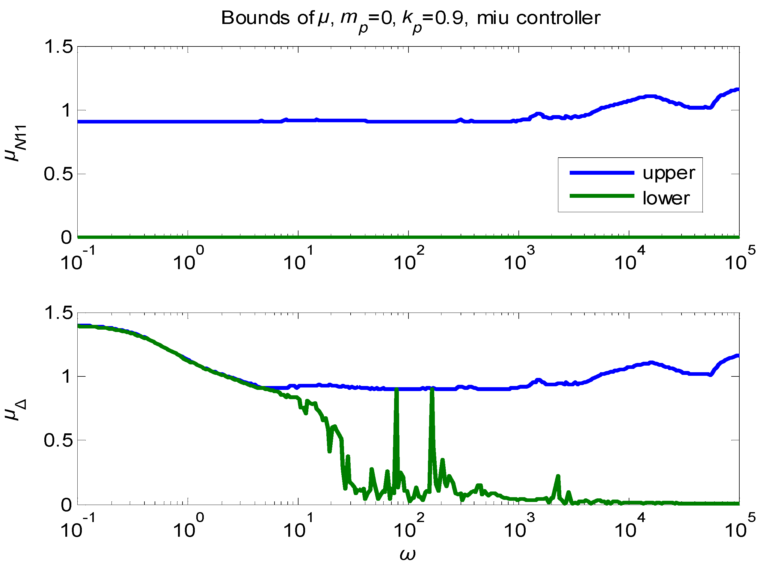
Figure 2 shows the μ-values of the computed controller’s μ-values. The majority of the frequencies indicate that the controller is reliable [8,9,10,11,12]. A higher μ-value indicates better system performance and robustness. One way to create a μ-controller is to use the D-K iteration process. As previously mentioned, this is an approximation process that provides boundaries for the μ-value.
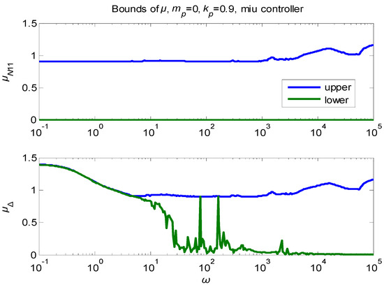
Figure 2.
The μ-controller’s boundaries for mp = 0 and kp = ±0.9.
Figure 3 illustrates a comparison of μ-controller performance at the free end, which serves as an indicator of the overall effectiveness. It is clear that the μ-controller surpasses the others in performance, albeit at the expense of an increased control effort. In Figure 3, the upper part shows the displacement of the free end of the beam. The blue line represents the displacement for the open-loop configuration of the beam, which means without control; the red line represents the displacement with the controller with μ-analysis. The results were very good when vibration suppression was achieved. In Figure 3 (bottom window), we consider the control voltages for the free end of the beam with a maximum voltage of 50 Volt. Figure 4 (left window) confirms this result. This might be the result of numerical issues with the μ-controller computation caused by the poor condition number of the plant. Another possible reason could be the high order of the μ-controller. Further research is required in either event. A higher μ value indicates a better robustness against uncertainties. The control system design using μ-analysis involves optimizing the controller to maximize μ and ensure robust stability and performance in the presence of uncertainties.
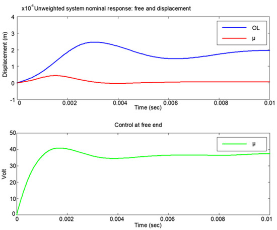
Figure 3.
Comparing the free-end data for the μ-controller (mp = 0, kp = ±0.9) in the nominal system.
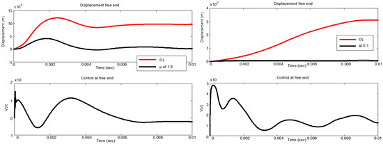
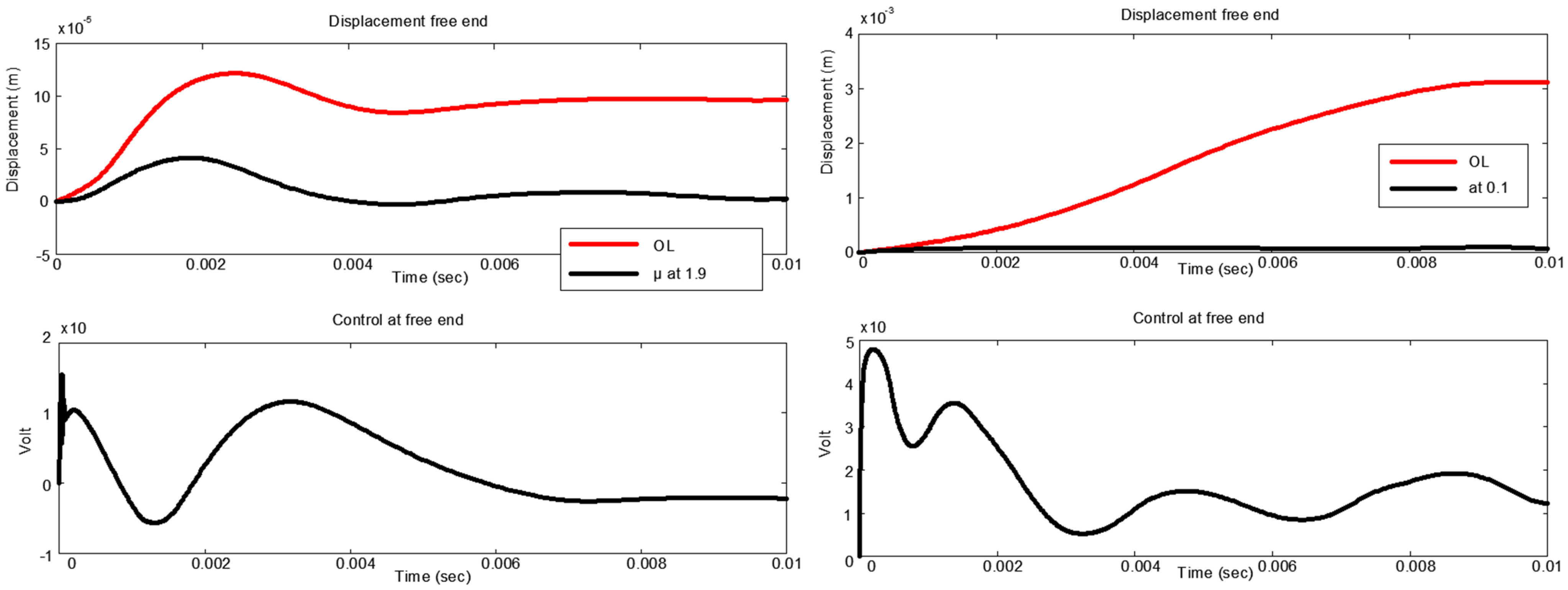
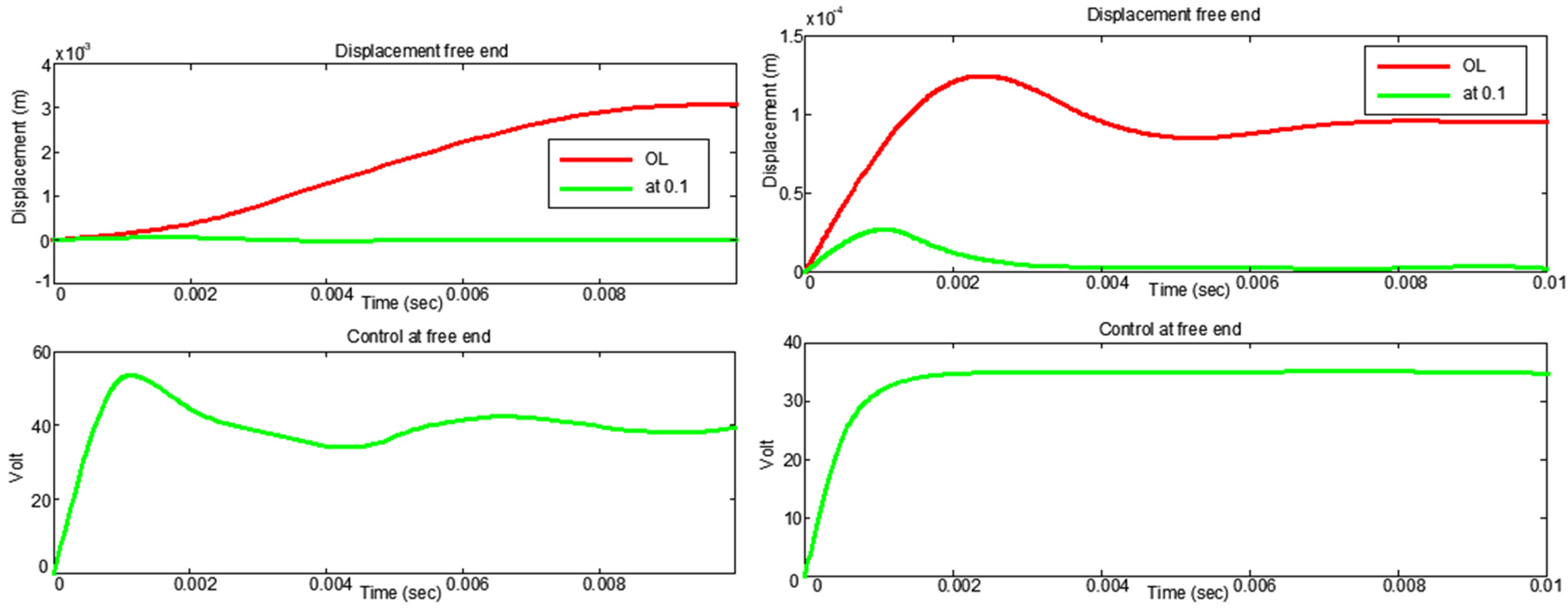
Figure 4.
Using mp = 0, kp = ±0.9, and control and displacement for the μ-controller at the free end.
Applying μ-analysis to smart structures involves considering uncertainties in the structural parameters and control elements and designing controllers that maximize μ to enhance robustness.
Figure 4 illustrates the displacement of the beam’s free end; the red line represents the displacement for the open loop of the beam, which means without control; the black line represents the displacement for the controller with μ-analysis. The results were very good when vibration suppression was achieved. In the bottom-left window, we take the control voltages for the free end of the beam with a maximum voltage of 15 Volt (Figure 4 bottom-left). The previous results are with Ko = 1.9 K: when Ko = 0.1 K (this translates to a ±90% deviation from the nominal value of the stiffness matrix K), the control voltages are 50 Volt (right down), and the displacement for the free end of the beam with and without control is shown in Figure 4 (upper-right window).
Moreover, mp = ±0.9 and kp = 0, which corresponds to a ±90% variation from the nominal.
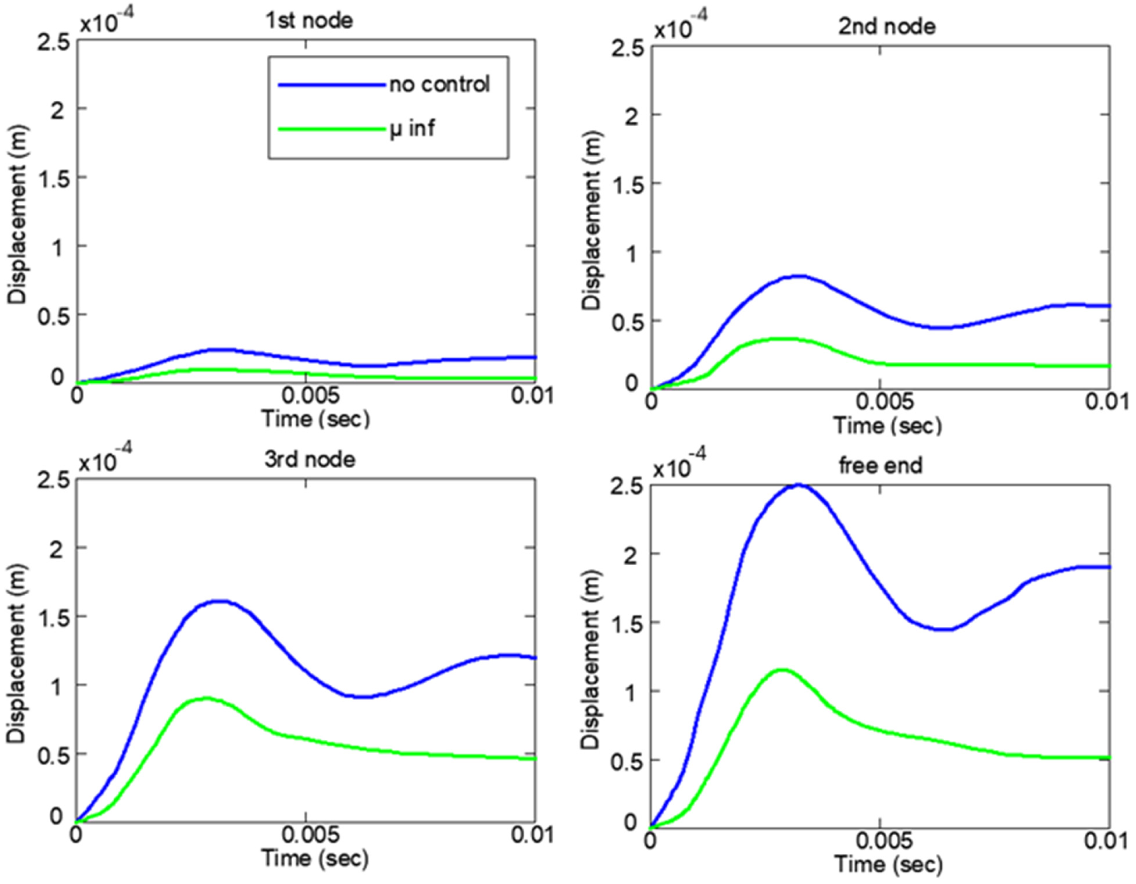
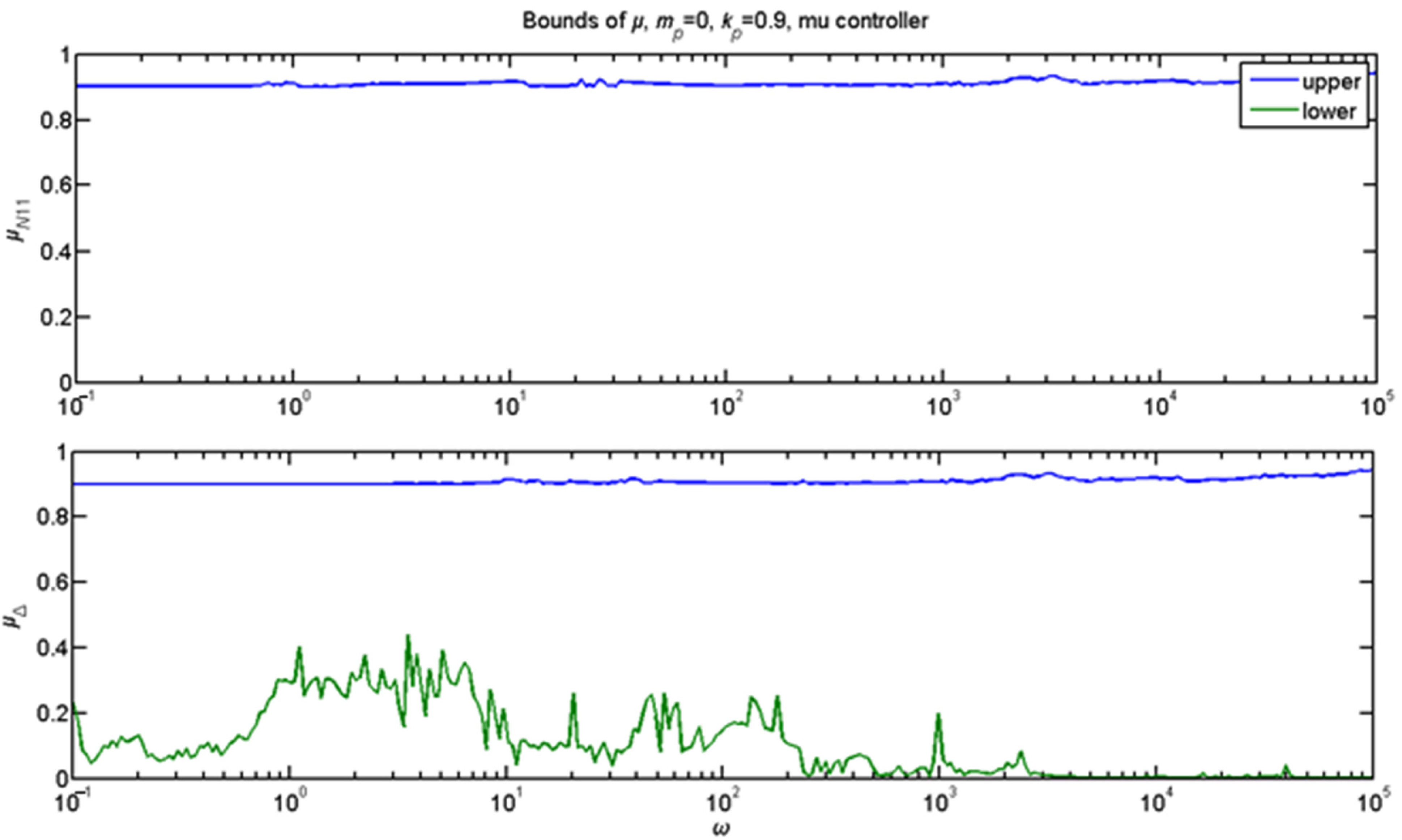
The displacement responses of this controller for the first mechanical input are shown in Figure 5. We take the results for the four nodes of the beam, and the results with the blue line are for the open loop, i.e., without control. The results with the green line are for μ-analysis, and the results with the μ-analysis are much better as we successfully rejected the oscillations. The previous results were in the state-space and frequency domains. The boundaries of the μ values are shown in Figure 6. As can be seen, the system continues to function robustly and steadily because the upper limits of both values remain below 1 for all relevant frequencies. This finding is confirmed in Figure 7, where the applied voltage and free-end movement are displayed at the maximum degree of uncertainty. The nominal controller performed better than the open-loop response for the identical system value of the stiffness matrix M.
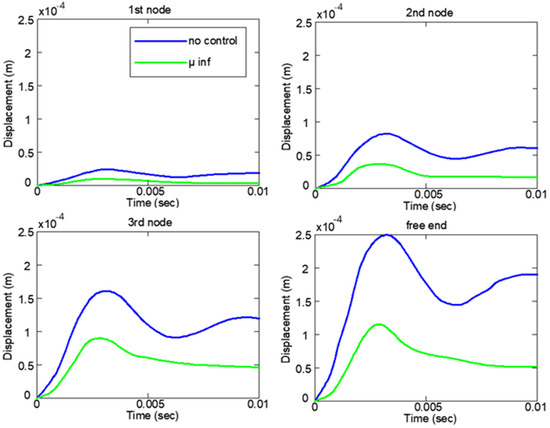
Figure 5.
Displacement response, μ-controller for kp = 0, mp = ±0.9, and 10 N at the free end.

Figure 6.
Limits of the μ-controller for mp = ±0.9 and kp = 0.
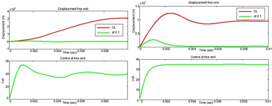
Figure 7.
Control and displacement at the free end for the μ-controller with extreme values mp = ±0.9 and kp = 0.
The top left of Figure 7 shows the displacement of the beam’s free end; the red line shows the displacement for the open loop of the beam, which means without control; and the green line shows the displacement with the controller with μ-analysis. The results were excellent, and vibration suppression was achieved. In the bottom-left window of Figure 7, we take the control voltages for the free end of the beam with a maximum voltage of 50 Volt. The previous results are for Mo = 1.9 K (this refers to a +90% variation from the nominal value of the mass matrix M), and the control voltages are 35 Volt (Figure 7, bottom right). The displacement at the beam’s free end both with and without control is shown in the upper-right window in Figure 7.
3.3. Reduced-Order Control
Because the presented controller has good results but has a very high order (56), an attempt was made to reduce the controller’s order using the Matlab package Hifoo (Mathworks, Natick, MA, USA), where the controller’s order is 2. The controller order was predetermined to be less than the plant order. Owing to the non-convexity and non-smoothness of the objective function, this optimization issue is challenging. Using a hybrid method based on many techniques, Hifoo searches for fixed-order controllers that achieve the minimal closed-loop H∞ norm in nonsmooth, nonconvex optimization [5,17,40].
The previous section addressed nonconvex and nonsmooth objective functions. Moreover, it can often be a situation in which the objectives cannot be distinguished by the local minimizers. The Hanso support package utilizes a hybrid algorithm to locally optimize the functions of this type. It consists of the following phases: an initial quasi-Newton algorithm (BFGS) phase that, unexpectedly, usually functions fairly effectively even in the presence of non-smoothness when applied using a suitable line search, and it frequently proposes an efficient method to estimate a local minimizer, a local bundle phase that attempts to confirm locally and optimality for the best point identified using BFGS and, if this malfunctions, a gradient sampling phase [40]. The use of gradients is required. The gradients of every optimization objective function supported using Hifoo can be easily computed using eigenvector or singular vector data that were previously acquired during the objective function computation process. Hanso receives these gradients, which are calculated using the Hifoo algorithm. There has been no attempt to locate unusual places when gradients are not present. The algorithms do not seem to be diverted by the areas of discontinuity in the gradients at exceptional places, or, in other words, in cases where the gradients cannot be found in these locations (which usually include optimizers). However, some algorithms use these discontinuities [40].
Additionally, all simulations are performed in MATLAB Simulink (Mathworks, Natick, MA, USA), including the block diagram in MATLAB Simulink (Mathworks, Natick, MA, USA), which is shown in Figure 8a. For all simulations, we discovered that noise, as a percentage, is ±2% of the disturbance (Figure 8b). The results are for the displacements and rotations of the smart beam nodes.
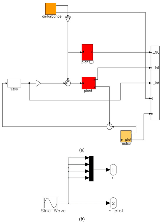
Figure 8.
(a) The block diagram in Matlab Simulink for the smart beam disturbance rejection with Hifoo controller and sinusoidal disturbance. (b) The block diagram in Matlab Simulink for the smart beam with sinusoidal noise (percentage ± 2% of the disturbance).
3.4. Problem Formulation and Optimization
The equations of the state space of a generalized plant G provide more details on the method with Hifoo.
and state-space realization of the controller K(s) is:
the matrices in our problem with the cantilever smart structure are
where A ∈ Rn×n, D12 ∈ Rp1×m2, and D21 ∈ Rp2×m1 have additional matrices of equivalent dimensions, and AK ∈ RnK×nK, with BK, CK, DK, AK, and the size of the generalized plant matrices are comparable. This constant order of control makes it identifiable to the designer. The measured inputs (or sensor inputs), control inputs, external inputs (such as disturbances and instructions), and controlled outputs are represented by the signals (z, w, y, and u) in that order. The symbol represents the transfer function Tzw from the input w to the output z (see [23] for further details). The optimal infinity controller design can be represented by minimizing the closed-loop H∞ characteristic function [41,42,43,44].
Inf ǁTzwǁ∞,
Kstabilizing
In accordance with this constraint, K(s) internally maintains the closed-loop system.
In this study, we implemented the additional criterion that the controller must be stable enough to reduce:
Inf ǁTzwǁ∞,
K stabilizing and K stable
To express the largest real component of the eigenvalues, or the spectral abscissa of matrix X, we use (X). Therefore, if the ACL is a closed-loop system matrix, both α(ACL) < 0 and α(AK) < 0 are required. The feasible set for AK, which is a set of stable matrices, has a ragged border and is not convex. It has been the subject of much investigation (see, for instance, [4,5,6]).
Similar to previous versions [6,40], Hifoo uses two processes: performance optimization and stability. Hifoo 2 continues to minimize max(α(ACL, ūα(AK)), a positive parameter that will lead to the subsequent detainment of additional information, as the closed-loop system remains stable once it locates a controller K wherein this number is negative, demonstrating that the controller is stabilized. An output indicating its inability to find a compatible controller was returned using Hifoo.
Regarding speed optimization, Hifoo 2 looks for a local minimizer in the following stages.
where:
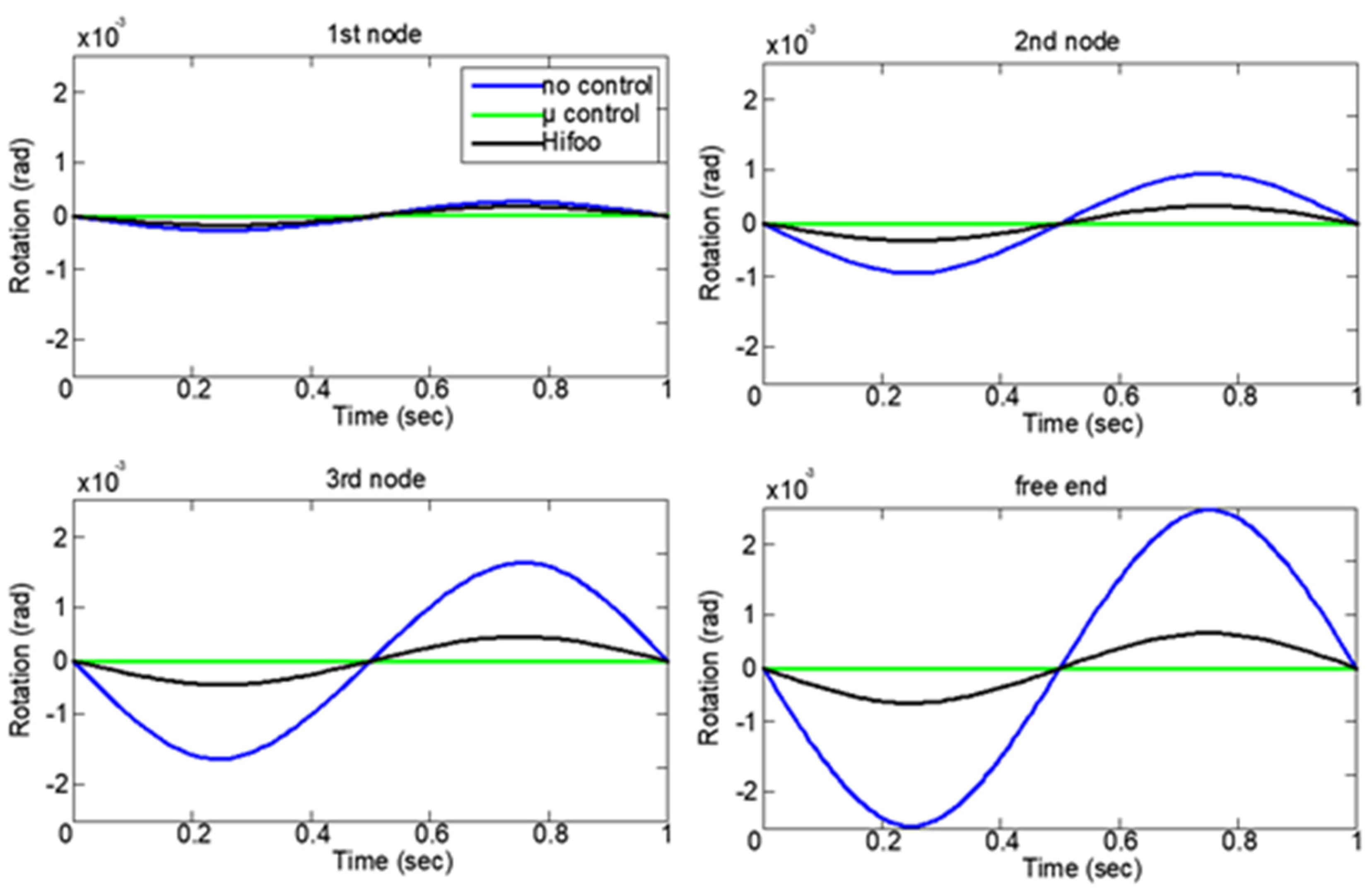
In Figure 9 and Figure 10, we can see the comparison with μ-analysis and the reduced-order control (Hifoo control) for all the nodes of the smart structure. Figure 9 shows the rotations for the four nodes of the structure, and Figure 10 shows the displacements. The results without control for the open loop are indicated by the blue line, the results with reduced-order control Hifoo are indicated by the black line, and the results with μ-analysis are indicated by the green line. The results are satisfactory, suppression of oscillations is achieved for dynamic loading, and both models of the control have very good results; meanwhile, the μ-analysis achieves a control model with almost zero displacement and rotation. Displacement rejection in smart structures refers to the ability of a structure to minimize or reject unwanted displacements in response to external forces or disturbances. This is a crucial aspect in the control system design for smart structures, especially in applications where precise positioning or stability is required. Displacement rejection was achieved in our study in both the μ-analysis and Hifoo control, employing a well-designed robust control system. Smart structures can actively counteract disturbances, maintain stability, and achieve precise control over their displacement, making them suitable for applications such as vibration suppression with robust criteria and structural positioning.

Figure 9.
The four nodes of the beam rotations with and without μ-analysis: rotation.
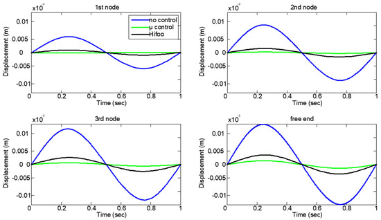
Figure 10.
The four nodes of the beam rotations with and without μ-analysis: displacement.
4. Discussion
The integration of active control, such as μ-analysis technologies, into smart structures has been the subject of the present work [4,36,40]. When utilizing the Hifoo controller in tandem with non-parametric and non-convex optimization methodologies, it ensures that the control output does not surpass operational constraints despite the desirable characteristics of low steady-state errors, rapid recovery, minimal maximum uplift, and reduced vibration, as outlined in [34,35,45].
The steps were as follows: 1. Determining the damping and stiffness. Mass and matrices using the finite element method. 2. Introduction of electrical charge and mechanics to the dynamic oscillation (Equation (3)). Application of control theory for modeling displacement results for finite element models with and without robust control. 4. Derivation of stress results using piezoelectric patches as actuators. 5. Decreasing the controller rank leads to a reduction in the computational requirements of the model. Remarkably, the controller demonstrated effective operation even with a significantly lower system degree.
Robust stabilization requires a self-stabilizing controller, whereas simultaneous stabilization requires the identification of a single controller. There are particular cases of multi-objective robust control challenges for stabilizing multiple plants [46,47,48,49]. Many of the current techniques and heuristics employed to address these issues often result in excessively high-order controllers. The results show the significant benefits of the proposed model and approach, and the control behavior of the beam aligns with our expectations. μ-Analysis is a technique used for analyzing and designing controllers for linear time-invariant systems. It deals with the frequency domain and helps to assess the robustness and performance of a control system. The goal is to find a controller that can handle uncertainties and variations in the system while maintaining stability and desired performance.
By contrast, HIifoo control is a method used in control theory that involves the design of controllers to achieve optimal performance in the presence of disturbances and uncertainties. Hifoo controllers are designed to minimize the impact of disturbances and uncertainties on the system output while meeting certain performance specification bounds [7,18,19,45].
In essence, μ-analysis is a broader technique for system analysis and controller design, while the Hifoo control is a specific approach within that broader framework, focused on achieving optimal performance in the presence of uncertainties. Control theory uses synthesis approaches to create controllers that provide guaranteed stability [48,49].
In the context of smart structures, μ-synthesis is a valuable tool for designing robust controllers that can effectively control the behavior of these structures, particularly when faced with uncertainties, variations, or disturbances. Smart structures typically involve the integration of sensors and actuators to respond actively to external stimuli and optimize their performance. In this context, μ-synthesis can be applied in the context of smart structures, which are often subjected to external disturbances such as wind, vibrations, or other environmental factors. We use μ-synthesis to design controllers that can reject these disturbances and maintain the desired structural performance. A control designer can use μ-analysis approaches to formulate the control issue as a mathematical optimization problem and then determine the controller that overcomes this optimization. One benefit of reduced-order approaches over conventional control methods is their ease of adaptation to multivariate systems with channel cross-coupling. The mathematical sophistication needed for effective application and the need for a reasonably precise model of the system to be managed are two disadvantages of the Hifoo approach. Note that the resulting controller is only optimal in terms of the necessary cost function and may not always be the best [48,49]. Hifoo approaches can be used to lessen the effect of a disturbance on a closed loop; the impact is evaluated in terms of performance or stability, depending on how the problem is formulated.
The experimental arrangement is part of our future plans, while the application of these materials has been demonstrated in aeronautics, mainly in the wings of airplanes, which can be considered cantilevers, as in the present model. The novelty of our study is that we succeeded in suppressing the oscillations caused by wind loads with small voltages. This is very important, that is, oscillation damping is a key problem in the field of mechanics. The major innovation of this study was the complete suppression of oscillations using advanced control techniques. The implementation of control is very difficult because modeling uncertainty is also introduced, that is, carrier imperfections and loading uncertainties.
5. Conclusions
The study presented herein advances the application of robust control to minimize oscillations in intelligent structures. The primary breakthrough lies in achieving the complete suppression of oscillations through the utilization of a lower-order controller. A reasonable repercussion of the proposed research achievements is the recognition of novel scientific problems that can provide a basis for investigations outside the scope of this work. The results of this effort are as follows: The time-space and frequency domains are acquired by reducing the order of oscillation suppression, leveraging the measurement noise of the beam state, introducing white noise input as a disturbance input, and interpreting it as a fraction of the disturbances, along with implementing the measurement noise. Additional impacts include the reduction in controller order, optimization of the μ-controller in intelligent structures, and control of oscillation suppression through intelligent entity simulation. Positive outcomes are derived from our use of μ-control and lower-order control to fully reject disruptions. Several control strategies used in structures to reduce noise and vibrations are discussed in this study. Hifoo control is a specific method with micro-analysis, which is essentially a larger methodology for system analysis and controller design, with the goal of achieving the best possible performance in the presence of uncertainty. The benefit of μ-synthesis is its robustness: μ-synthesis provides a systematic approach for designing controllers that are robust against uncertainties, ensuring stable and satisfactory performance over a range of operating conditions.
Author Contributions
A.M. and M.P.: software, formal analysis, writing review, and editing; G.E.S.: methodology; A.P.: investigation, software; N.V.: validation. All authors have read and agreed to the published version of the manuscript.
Funding
This study received no external funding.
Data Availability Statement
The data presented in this study are available upon request from the corresponding authors.
Conflicts of Interest
The authors declare no conflicts of interest.
Appendix A
MATLAB code:
% uncertainty analysis
mpp = 0
kpp = 0.9
delta_m =0
delta_k = 1
percn = kpp*100
% % bw1 = ureal(‘bw1’, 1, ‘Percentage’, percn, ‘autosimplify’, ‘full’)
bw1 = 1
bw2 = ureal(‘bw2’, 1, ‘Percentage’, percn, ‘autosimplify’, ‘full’)
ex_un = 1 + percn/100
E1 = [zeros(nd, nd) eye(nd);
eye(nd) zeros(nd, nd);
zeros(nd, 2*nd)];
E2 = [ zeros(nd, 2*nd)
zeros(nd, 2*nd)
eye(nd) zeros(nd, nd)];
delta_un = [eye(nd)*delta_m zeros(nd);
zeros(nd) eye(nd)*delta_k];
Gbar = -[mm1*mpp kk1*kpp];
Gbar0 = [zeros(nd, 2*nd);
invM*Gbar];
Gbar1 = [eye(nd) 0.0005*eye(nd) zeros(nd);
zeros(nd) 0.0005*eye(nd) eye(nd)];
Wm = Gbar0*delta_un*Gbar1;
References
- Benjeddou, A.; Trindade, M.A.; Ohayon, R. New Shear Actuated Smart Structure Beam Finite Element. AIAA J. 1999, 37, 378–383. [Google Scholar] [CrossRef]
- Bona, B.; Indri, M.; Tornambe, A. Flexible Piezoelectric Structures-Approximate Motion Equations and Control Algorithms. IEEE Trans. Autom. Control 1997, 42, 94–101. [Google Scholar] [CrossRef]
- Okko, B.; Kwakernaak, H.; Gjerrit, M. Design Methods for Control Systems; Dutch Institute of Systems and Control: Delft, The Netherlands, 2001. [Google Scholar]
- Burke, J.V.; Henrion, D.; Lewis, A.S.; Overton, M.L. Stabilization via Nonsmooth, Nonconvex Optimization. IEEE Trans. Autom. Control 2006, 51, 1760–1769. [Google Scholar] [CrossRef]
- Burke, J.V.; Lewis, A.S.; Overton, M.L. A Robust Gradient Sampling Algorithm for Nonsmooth, Nonconvex Optimization. SIAM J. Optim. 2005, 15, 751–779. [Google Scholar] [CrossRef]
- Burke, J.V.; Overton, M.L. Variational Analysis of Non-Lipschitz Spectral Functions. Math. Program. 2001, 90, 317–351. [Google Scholar] [CrossRef]
- Choi, S.-B.; Cheong, C.-C.; Lee, C.-H. Position Tracking Control of a Smart Flexible Structure Featuring a Piezofilm Actuator. J. Guid. Control Dyn. 1996, 19, 1364–1369. [Google Scholar] [CrossRef]
- Hanagud, S.; Obal, M.W.; Calise, A.J. Optimal Vibration Control by the Use of Piezoceramic Sensors and Actuators. J. Guid. Control Dyn. 1992, 15, 1199–1206. [Google Scholar] [CrossRef]
- Song, G.; Sethi, V.; Li, H.-N. Vibration Control of Civil Structures Using Piezoceramic Smart Materials: A Review. Eng. Struct. 2006, 28, 1513–1524. [Google Scholar] [CrossRef]
- Karatzas, I.; Lehoczky, J.P.; Shreve, S.E.; Xu, G.-L. Modeling, Control and Implementation of Smart Structures: A FEM-State Space Approach; Springer: Berlin/Heidelberg, Germany, 1990; ISBN 9783540483939. [Google Scholar]
- Miara, B.; Stavroulakis, G.; Valente, V. Topics on Mathematics for Smart Systems. In Proceedings of the European Conference, Rome, Italy, 26–28 October 2006. [Google Scholar]
- Moutsopoulou, A.; Stavroulakis, G.E.; Pouliezos, A.; Petousis, M.; Vidakis, N. Robust Control and Active Vibration Suppression in Dynamics of Smart Systems. Inventions 2023, 8, 47. [Google Scholar] [CrossRef]
- Zhang, X.; Shao, C.; Li, S.; Xu, D.; Erdman, A.G. Robust H∞ Vibration Control for Flexible Linkage Mechanism Systems with Piezoelectric Sensors And Actuators. J. Sound Vib. 2001, 243, 145–155. [Google Scholar] [CrossRef]
- Li, C.; Liang, M. A Generalized Synchrosqueezing Transform for Enhancing Signal Time–Frequency Representation. Signal Process. 2012, 92, 2264–2274. [Google Scholar] [CrossRef]
- Li, Z.; Adeli, H. New Adaptive Robust H∞ Control of Smart Structures Using Synchrosqueezed Wavelet Transform and Recursive Least-Squares Algorithm. Eng. Appl. Artif. Intell. 2022, 116, 105473. [Google Scholar] [CrossRef]
- Li, Z.; Adeli, H. New Discrete-Time Robust H2/H∞ Algorithm for Vibration Control of Smart Structures Using Linear Matrix Inequalities. Eng. Appl. Artif. Intell. 2016, 55, 47–57. [Google Scholar] [CrossRef]
- Burke, J.V.; Henrion, D.; Lewis, A.S.; Overton, M.L. Hifoo—A MATLAB package for fixed-order controller design and H∞ optimization. IFAC Proc. Vol. 2006, 39, 339–344. [Google Scholar] [CrossRef]
- Culshaw, B. Smart Structures—A Concept or a Reality? Proc. Inst. Mech. Eng. Part I J. Syst. Control Eng. 1992, 206, 1–8. [Google Scholar] [CrossRef]
- Doyle, J.; Glover, K.; Khargonekar, P.; Francis, B. State-Space Solutions to Standard H2 and H∞ Control Problems. In Proceedings of the 1988 American Control Conference, Atlanta, GA, USA, 15–17 June 1988; pp. 1691–1696. [Google Scholar]
- Tzou, H.S.; Gabbert, U. Structronics—A New Discipline and Its Challenging Issues. Fortschr. Berichte VDI Smart Mech. Syst. Adapt. Reihe 1997, 11, 245–250. [Google Scholar]
- Tzou, H.S.; Anderson, G.L. Intelligent Structural Systems; Springer: Dordrecht, The Netherlands; Boston, MA, USA; London, UK, 1992; ISBN 978-94-017-1903-2. [Google Scholar]
- Guran, A.; Tzou, H.-S.; Anderson, G.L.; Natori, M.; Gabbert, U.; Tani, J.; Breitbach, E. Structronic Systems: Smart Structures, Devices and Systems; WORLD SCIENTIFIC: Singapore, 1998; Volume 4, ISBN 978-981-02-2652-7. [Google Scholar]
- Gabbert, U.; Tzou, H.S. IUTAM Symposium on Smart Structures and Structronic Systems. In Proceedings of the IUTAM Symposium, Magdeburg, Germany, 26–29 September 2000; Kluwer: Dordrecht, The Netherlands; Boston, MA, USA; London, UK, 2001. [Google Scholar]
- Tzou, H.S.; Natori, M.C. Piezoelectric Materials and Continua; Braun, S.B.T.-E.V., Ed.; Elsevier: Oxford, UK, 2001; pp. 1011–1018. ISBN 978-0-12-227085-7. [Google Scholar]
- Cady, W.G. Piezoelectricity: An Introduction to the Theory and Applications of Electromechanical Phenomena in Crystals; Dover Publication: New York, NY, USA, 1964. [Google Scholar]
- Tzou, H.S.; Bao, Y. A Theory on Anisotropic Piezothermoelastic Shell Laminates with Sensor/Actuator Applications. J. Sound Vib. 1995, 184, 453–473. [Google Scholar] [CrossRef]
- Moutsopoulou, A.; Stavroulakis, G.E.; Petousis, M.; Vidakis, N.; Pouliezos, A. Smart Structures Innovations Using Robust Control Methods. Appl. Mech. 2023, 4, 856–869. [Google Scholar] [CrossRef]
- Cen, S.; Soh, A.-K.; Long, Y.-Q.; Yao, Z.-H. A New 4-Node Quadrilateral FE Model with Variable Electrical Degrees of Freedom for the Analysis of Piezoelectric Laminated Composite Plates. Compos. Struct. 2002, 58, 583–599. [Google Scholar] [CrossRef]
- Packard, A.; Doyle, J.; Balas, G. Linear, Multivariable Robust Control with a μ Perspective. J. Dyn. Syst. Meas. Control 1993, 115, 426–438. [Google Scholar] [CrossRef]
- Kim, S.-W.; Boo, C.-J.; Kim, S.; Kim, H.-C. Stable Controller Design of MIMO Systems in Real Grassmann Space. Int. J. Control Autom. Syst. 2012, 10, 213–226. [Google Scholar] [CrossRef]
- Feng, Z.; Allen, R. Reduced Order H∞ Control of an Autonomous Underwater Vehicle. IFAC Proc. Vol. 2003, 36, 121–126. [Google Scholar] [CrossRef]
- Chandrashekhara, K.; Varadarajan, S. Adaptive Shape Control of Composite Beams with Piezoelectric Actuators. J. Intell. Mater. Syst. Struct. 1997, 8, 112–124. [Google Scholar] [CrossRef]
- Ackermann, J. Robust Control, The Parameter Space Approach; Springer: London, UK, 2002; ISBN 978-1-85233-514-4. [Google Scholar]
- Vidakis, N.; Petousis, M.; Mountakis, N.; Papadakis, V.; Moutsopoulou, A. Mechanical Strength Predictability of Full Factorial, Taguchi, and Box Behnken Designs: Optimization of Thermal Settings and Cellulose Nanofibers Content in PA12 for MEX AM. J. Mech. Behav. Biomed. Mater. 2023, 142, 105846. [Google Scholar] [CrossRef] [PubMed]
- Kwakernaak, H. Robust Control and H∞-Optimization—Tutorial Paper. Automatica 1993, 29, 255–273. [Google Scholar] [CrossRef]
- Blondel, V.D.; Tsitsiklis, J.N. A Survey of Computational Complexity Results in Systems and Control. Automatica 2000, 36, 1249–1274. [Google Scholar] [CrossRef]
- Gao, H.; Lam, J.; Wang, C. Controller Reduction with Error Performance: Continuous- and Discrete-Time Cases. Int. J. Control 2006, 79, 604–616. [Google Scholar] [CrossRef]
- Yang, S.M.; Lee, Y.J. Optimization of Noncollocated Sensor/Actuator Location and Feedback Gain in Control Systems. Smart Mater. Struct. 1993, 2, 96. [Google Scholar] [CrossRef]
- Ramesh Kumar, K.; Narayanan, S. Active Vibration Control of Beams with Optimal Placement of Piezoelectric Sensor/Actuator Pairs. Smart Mater. Struct. 2008, 17, 55008. [Google Scholar] [CrossRef]
- Burke, J.V.; Lewis, A.S.; Overton, M.L. A Nonsmooth, Nonconvex Optimization Approach to Robust Stabilization by Static Output Feedback and Low-Order Controllers. IFAC Proc. Vol. 2003, 36, 175–181. [Google Scholar] [CrossRef]
- Leibfritz, F. COMPleib: COnstrained Matrix-Optimization Problem Library—A Collection of Test Examples for Nonlinear Semidefinite Programs, Control System Design and Related Problems; University of Trier: Trier, Germany, 2006; pp. 1–23. [Google Scholar]
- Wie, B.; Bernstein, D.S. Benchmark Problems for Robust Control Design. J. Guid. Control Dyn. 1992, 15, 1057–1059. [Google Scholar] [CrossRef]
- Henrion, D.; Overton, M.L. Maximizing the Closed Loop Asymptotic Decay Rate for the Two-Mass-Spring Control Problem. arXiv 2006, arXiv:math/0603681. [Google Scholar]
- Henrion, D.; Sebek, M. Overcoming Non-Convexity in Polynomial Robust Control Design. In Proceedings of the 16th International Symposium on Mathematical Theory of Networks and Systems, Leuven, Belgium, 1 January 2004. [Google Scholar]
- Zhang, N.; Kirpitchenko, I. Modelling Dynamics of A Continuous Structure with a Piezoelectric Sensoractuator for Passive Structural Control. J. Sound Vib. 2002, 249, 251–261. [Google Scholar] [CrossRef]
- Stavroulakis, G.E.; Foutsitzi, G.; Hadjigeorgiou, E.; Marinova, D.; Baniotopoulos, C.C. Design and Robust Optimal Control of Smart Beams with Application on Vibrations Suppression. Adv. Eng. Softw. 2005, 36, 806–813. [Google Scholar] [CrossRef]
- Kimura, H. Robust Stabilizability for a Class of Transfer Functions. IEEE Trans. Autom. Control 1984, 29, 788–793. [Google Scholar] [CrossRef]
- Francis, B.A. A Course in H∞ Control Theory; Springer: Berlin/Heidelberg, Germany, 1987; ISBN 978-3-540-17069-3. [Google Scholar]
- Moutsopoulou, A.; Petousis, M.; Vidakis, N.; Stavroulakis, G.E.; Pouliezos, A. Applications of the Order Reduction Optimization of the H-Infinity Controller in Smart Structures. Inventions 2023, 8, 150. [Google Scholar] [CrossRef]


Disclaimer/Publisher’s Note: The statements, opinions and data contained in all publications are solely those of the individual author(s) and contributor(s) and not of MDPI and/or the editor(s). MDPI and/or the editor(s) disclaim responsibility for any injury to people or property resulting from any ideas, methods, instructions or products referred to in the content. |
© 2024 by the authors. Licensee MDPI, Basel, Switzerland. This article is an open access article distributed under the terms and conditions of the Creative Commons Attribution (CC BY) license (https://creativecommons.org/licenses/by/4.0/).