Group Dynamics in Memory-Enhanced Ant Colonies: The Influence of Colony Division on a Maze Navigation Problem

Abstract

This paper introduces an agent-based model grounded in the ACO algorithm to investigate the impact of partitioning ant colonies on algorithmic performance. The exploration focuses on understanding the roles of group size and number within a multi-objective optimization context. The model consists of a colony of memory-enhanced ants (ME-ANTS) which, starting from a given position, must collaboratively discover the optimal path to the exit point within a grid network. The colony can be divided into groups of different sizes and its objectives are maximizing the number of ants that exit the grid while minimizing path costs. Three distinct analyses were conducted: an overall analysis assessing colony performance across different-sized groups, a group analysis examining the performance of each partitioned group, and a pheromone distribution analysis discerning correlations between temporal pheromone distribution and ant navigation. From the results, a dynamic correlation emerged between the degree of colony partitioning and solution quality within the ACO algorithm framework.

1. Introduction

Network analysis is typically understood as a collection of methodologies and heuristics that allow us to understand the relationships among entities within complex systems. Network analysis finds application in human fields such as sociology [1,2], economics [3,4,5], biology [6,7], medicine [8,9], and many others. For example, in sociology, network analysis can identify online communities [10,11] and social interactions [12] or measure social influence within a friendship network. In economics, we can analyze business relationships and understand how the interconnection between companies affects market stability. In biology, we can study interactions between proteins within cells to better understand biological mechanisms [13,14].

In this paper, we delve into a specific aspect of network analysis within the framework of an Ant Colony Optimization (ACO) algorithm, focusing on the dynamic relationships and interactions among individual ants and various groups within a colony. The colony functions as a complex network, where ants collaborate to find the optimal path between a food source and their nest, communicating through a simple yet indirect mechanism using chemical signals known as pheromones. This phenomenon serves as a prime example of a complex adaptive system (CAS), where the collective behavior transcends the actions of individual elements, showing the colony’s ability to thrive through cooperation [15]. In essence, it is not the solitary ant that discovers the optimal path, but rather the intricate interactions among groups of ants within the colony, facilitated by pheromones, that yield the overall outcome [16]. Our exploration delves into the interactions through pheromones and the structural organization of the colony. By analyzing how various forms of grouping, coupled with factors such as pheromone evaporation, influence intra-colony relations, we aim to comprehensively grasp the diverse outcomes generated by the algorithm in question. Consequently, our investigation extends beyond the realm of pheromone-driven interactions to encompass the substantial impact of colony subdivision on the overall dynamics.

1.1. The ACO Paradigm and Applications

Ant Colony Optimization (ACO) derives its inspiration from the foraging behavior observed in natural ant colonies, where decentralized communication through chemical signals known as pheromones plays a pivotal role in finding the shortest path between their nest and a source of food. Initially proposed in [17], ACO has demonstrated remarkable efficacy in addressing a multitude of complex combinatorial optimization problems, including scheduling and, particularly, routing problems [18,19,20,21,22,23]. More generally speaking, agent-based or swarm intelligence heuristics have been applied as well to coloring challenges [24,25,26], robot path planning for inaccessible areas [27,28], transportation complexities and traffic problems [29,30], and feature selection across diverse fields [31]. Beyond optimization, ACO demonstrates utility in modeling crowd dynamics. In [32], the authors translated ACO rules into conceptual frameworks rooted in social dynamics. They proposed an agent-based model to study collective crowd behaviors. Furthermore, ref. [33] provides a sensitivity analysis.

The notion of dividing ant colonies into groups has received particular attention because of its potential to enhance optimization performance. In [34], an adaptive ACO was implemented, where the colony was separated into three groups: ordinary ants, using heuristic information; abnormal ants, seeking low pheromone paths; and random ants, exploring randomly. This collaborative approach improved the optimization performance, and was able, for instance, to effectively address the traveling salesman problem.

Extending this exploration into multi-objective optimization problems, ref. [35] emphasized the performance benefits of employing multiple ant groups. In their study, a grouping approach was applied to enhance the efficacy of the ACO paradigm when dealing with multi-objective optimization problems.

In a related effort, ref. [36] proposed a multi-objective ACO algorithm for community detection in complex networks. By partitioning the ant colony into groups and coordinating their exploration, the algorithm achieved a more efficient search ability for solutions. Further corroborating these findings, Ref. [37] introduced a group-based ACO algorithm for bi-objective optimization, where ants were organized into groups based on parameters related to the objective function, resulting in an enhanced overall algorithm performance. Recent advancements include the Grouping Ant Colony Optimization (GACO) algorithm presented by [38]. GACO specifically addresses the multi-UAV reconnaissance task allocation problem by dividing the ant colony into distinct subgroups. This division proves crucial as different UAVs focus on distinct targets, ultimately leading to superior optimality in the results when compared to existing methods reported in the literature. Lastly, we stress the possibility of future applications of the GACO algorithm to networks modeling the mobility of groups of people, providing, for instance, personalized recommendations of places of interest [39] and possibly analyzing the impact of restrictions to mobility due to extreme circumstances [40].

Building upon the advancements in multi-objective optimization techniques, some recent studies have introduced innovative algorithms to address specific problems in different domains. For instance, in [30] the authors propose a modified Competitive Mechanism Multi-Objective Particle Swarm Optimization (MCMOPSO) algorithm for optimizing signalized traffic problems. This approach incorporates a dynamic leader selection mechanism, guiding particles toward elite solutions through angle comparisons. Similarly, in [41] a single deep reinforcement learning model is employed to tackle the multi-objective traveling salesman problem (MOTSP). The method makes use of an encoder–decoder framework with a routing encoder, efficiently extracting and aggregating information to generate approximate Pareto-optimal solutions in parallel.

1.2. Objective of Our Research

The exploration of dividing ant colonies into groups as a strategy to optimize Ant Colony Optimization (ACO) raises some compelling questions: what is the optimal degree of partitioning to achieve the best solution to the problem at hand? Are there any potential correlations between the solution quality and variables within the ACO framework? To address these questions, an agent-based model, rooted in the ACO paradigm but where the agents (ants) have memory, was employed to tackle a maze navigation problem. Drawing on insights from existing research, the present study investigates the impact of partitioning the colony into groups on the ACO algorithm’s performance, particularly examining the roles of group size and number in the context of a multi-objective optimization problem. The decision to adopt an agent-based approach is motivated by the necessity to explore the network dynamics inherent in the collaborative behaviors of the ant colony. In related studies [42], the same approach was used to explore the network dynamics of both collaborative and competitive ant colonies. The flexibility of this model proves crucial in capturing the complex and dynamic interactions within the colony, where each agent, representing an individual ant, interacts with the environment and each other. These interactions, facilitated by pheromones, lead to the emergence of collective behaviors, offering a deeper understanding of how the network evolves and adapts to changing conditions while exploring diverse scenarios.

In conclusion, the present study focuses on a dynamic scenario where a colony of memory-enhanced ants, starting from a designated position, collaboratively attempts to discover the optimal path to the exit within a grid network. The colony is divided into groups of varying sizes, with the overarching goal of maximizing the number of ants successfully exiting the maze while minimizing path costs.

The paper is structured as follows: Section 2 clarifies the model, offering a comprehensive understanding of it. In Section 3, the experimental setup and results of the experiments are provided. Section 4 critically discusses the obtained results. Finally, in Section 5 we present the concluding remarks.

2. The Model

We used the NetLogo software [43] to implement our model. NetLogo is an agent-based programming language as well as an integrated development environment (IDE) that provides a comprehensive environment, from the implementation of the simulation model to the creation of the graphical interface supporting the simulation. The graphical interface typically includes various elements such as switches, sliders, choosers, and inputs, chosen according to the user’s needs for model development. These elements allow a real-time interaction to observe changes in the dynamics without directly modifying the code. Interface elements can correspond to either simple model variables or code blocks and are arbitrary, as they may not be present for the model’s executability, as long as the associated variables or code are properly defined in the source code. The graphical interface must include two elements: one designed to invoke the code initializing the simulation environment (typically named “setup”), and another that calls the code initiating the dynamics (commonly labeled as “start”).

The environment is a weighted network defined as a graph $G=(V,E,w)$, where V is the set of vertices, E is the set of edges, and $w:V\times V\to {\mathbb{R}}^{+}$ is the weight function which assigns a positive cost to each edge of the graph. The weight measures the difficulty of crossing a specific edge. The starting point is a randomly selected node on one side (e.g., left side), while the exit point is another randomly chosen node on the opposite side (e.g., right side). The graph is undirected, therefore, all the edges can be crossed in both directions.

Let $A_i=\{j\in V:(i,j)\in E\}$ represent the set of vertices adjacent to vertex i and let ${\pi }^k\left(t\right)=({\pi }_1,{\pi }_2,\cdots ,{\pi }_t)$ denote the set of vertices visited by the ant k at a specific time t, where $({\pi }_i,{\pi }_{i+1})\in E$ for $i=1,\cdots ,t-1$. The probability $p_{ij}^k\left(t\right)$ which measures the likelihood that ant $k,$ placed on a vertex $i,$ chooses as destination one of its neighbor vertices j at time t is defined as

$$p_{ij}^k\left(t\right)=\left\{\begin{array}{cc}\frac{{\tau }_{ij}{\left(t\right)}^{\alpha }·{\eta }_{ij}^{\beta }}{{\sum }_{l\in J_i^k}{\tau }_{il}{\left(t\right)}^{\alpha }·{\eta }_{il}^{\beta }}\hfill & \mathrm{if}j\in J_i^k\hfill \\ 0\hfill & \mathrm{otherwise},\hfill \end{array}\right.$$

(1)

where $J_i^k=A_i\setminus \left\{{\pi }_t^k\right\}$ represents all the possible displacements of ant k from vertex i, ${\tau }_{ij}\left(t\right)$ is the pheromone intensity on edge $(i,j)$, and ${\eta }_{ij}\left(t\right)$ is the desirability of edge $(i,j)$ at a given time t. The parameters $\alpha$ and $\beta$ determine, respectively, the importance of pheromone intensity and the importance of the desirability of an edge. Each link undergoes asynchronous updates through two types of rules based on the number of ticks T (the tick is the unit of time in the simulation software). The first rule is a local updating rule, which adjusts the pheromone levels after each movement of the ant as follows:

$${\tau }_{ij}(t+1)={\tau }_{ij}\left(t\right)+K.$$

(2)

Here, K denotes the pheromone left by each ant after traversing an edge $(i,j)$, and ${\tau }_{ij}\left(t\right)$ represents the pheromone amount on the link at time t.

The second rule is a global updating rule, which updates the pheromone amount on all network links every T ticks as follows:

$$\begin{array}{c}\hfill {\tau }_{ij}(t+1)=(1-\rho )·{\tau }_{ij}\left(t\right),\end{array}$$

(3)

where ${\tau }_{ij}\left(t\right)$ is the trace amount on edge $(i,j)$ at time t, and $\rho$ is the evaporation decay parameter. At any given time t, the desirability ${\eta }_{ij}\left(t\right)$ measures the attractiveness of an edge $(i,j)$. This desirability is associated with the information $I_{ij}\left(t\right)$ about the weight of the edge. It is shared by each ant on the endpoint of the crossed edge $(i,j)$ and initialized to 0, as in Algorithm 1 line 3.

2.1. Memory-Enhanced Ants and Knowledge Acquisition

In our model, ants employ a navigation strategy that combines the use of pheromones and the calculated desirability of edges to make informed decisions about their movement within the environment. Pheromones act as a communication device among ants, directing them towards paths with higher concentrations of pheromones. Conversely, desirability is internally determined based on acquired information $I_{ij}\left(t\right)$ about edge weights, achieved through two mechanisms.

The first memory mechanism employed by ants involves traversing edges and storing the weights in their memory as prior knowledge ${\overline{w}}_p^k$. As ants explore their environment, they accumulate information about the weights of the edges they traverse. The prior knowledge represents the average weight of the visited edges, computed by summing the weights along a generic path ($\pi \left(t\right)$) and dividing by the number of edges in that path (n). This process, outlined in Equation (4), enables ants to establish a historical understanding of the environment. The prior knowledge mechanism allows ants to form preferences for certain paths based on their past experiences. In essence, this memory mechanism reflects the ants’ ability to internalize and use information about previously encountered paths, shaping their decision-making in navigating the environment.

$${\overline{w}}_p^k=\frac{1}{n}\sum _{i=1}^{n}w({\pi }_i,{\pi }_{i+1});$$

(4)

The second memory mechanism involves the acquisition of information about edge weights at the nearest endpoint, leading to the formation of their local knowledge ${\overline{w}}_l^k$. Ants discern information ($I_{ij}\left(t\right)$) about the weights of edges in their immediate vicinity, considering the number of neighboring edges (m) at the position where this information is present (Figure 1).

The local knowledge is then determined as the average weight of these neighboring edges, as expressed in Equation (5). This mechanism allows ants to adapt their decision-making based on real-time information acquired from their immediate surroundings. By considering the specific context at the nearest endpoint, ants enhance their awareness of the current environment and adjust their desirability calculations accordingly. The combination of prior knowledge and local knowledge mechanisms enables ants to strike a balance between past experience and current information, facilitating efficient navigation and adaptation to their dynamic surroundings,

$${\overline{w}}_l^k=\frac{1}{m}\sum _{i=1}^{m}w({\pi }_i,{\pi }_{i+1}).$$

(5)

The overall desirability value ${\eta }_{ij}\left(t\right)$ is then determined using a decision tree (Equation (6)), considering the availability of information $I_{ij}\left(t\right)$ and the type of knowledge:

$${\eta }_{ij}\left(t\right)=\left\{\begin{array}{cc}\frac{1}{w_{ij}}\hfill & \mathrm{if}{I}_{ij}\ne 0\mathrm{and}\mathrm{T}\ne 0\hfill \\ \frac{1}{\overline{w}}\hfill & \mathrm{if}{I}_{ij}=0\mathrm{and}\mathrm{T}\ne 0\hfill \\ 1\hfill & \mathrm{if}{I}_{ij}=0\mathrm{and}\mathrm{T}=0\hfill \end{array}\right.$$

(6)

The global knowledge ($\overline{w}$) is the mean of the prior and local knowledge:

$$\overline{w}=\frac{{\overline{w}}_p^k+{\overline{w}}_l^k}{2}.$$

(7)

When an ant is on a node i, it calculates ${\eta }_{ij}\left(t\right)$ considering the edge weight, with higher desirability for lower weights. If information $I_{ij}\left(t\right)$ is available at either nearest endpoint, the ant inversely relates desirability to the edge weight. In scenarios where information $I_{ij}\left(t\right)$ about neighboring edges is absent, the ant estimates desirability as the inverse of its global knowledge. This estimation is derived by averaging prior and local knowledge. Figure 2b illustrates this.

In cases of no prior and local knowledge, as depicted in Figure 2a, the ant assigns an equal desirability value of 1 to all edges.

In essence, as ants traverse edges, their prior and local knowledge contributes to the calculation of the desirability values. These values, representing the attractiveness of different paths, guide ants in choosing routes that align with both the pheromone trail and the desirability criteria. The combination of pheromone-based communication and desirability-driven decision-making allows the ants to navigate efficiently in a complex environment, adapting to changing conditions and optimizing their collective exploration.

The total path cost from the initial to the destination point is determined by the following expression:

$$\sum _{i=1}^{t-1}w({\pi }_i,{\pi }_{i+1}),$$

(8)

where ${\pi }_1$ and ${\pi }_t$ represent the starting and destination points, respectively.

2.2. Description of the ME-ANTS Algorithm

The ME-ANTS algorithm, whose pseudocode is given in Algorithm 1, takes as input a weighted graph $G(V,E,w)$, which represents the environment, with set of vertices V of size $\left|V\right|=m$, set of edges E, and edge weights w. It also takes as inputs several other parameters, namely, $\alpha$ and $\beta$, which determine the importance of pheromone intensity and edge desirability; K, which is the amount of pheromone released by each ant; $\rho$ is the evaporation rate; $T_d$ and $T_{max}$ represent the exit interval between groups and maximum simulation time; $A=\{a_1,a_2,\dots ,a_n\}$ is the set of ants, partitioned into g groups $S_1,\dots ,S_g$ of equal cardinality, with n being the total number of ants, g the number of groups, and $\Delta$ the collection of the g groups. The algorithm outputs two key values: num_exited, which denotes the number of ants successfully reaching the exit node, and path_cost, which is the average cost of the traversed paths.

Two matrices are used: P for pheromone levels and I as a Boolean matrix for information release. P is initialized with all entry values equal to 1, while I is initialized with all entry values equal to 0. I plays a crucial role in calculating edge $(v_i,v_j)$ desirability (${\eta }_{ij}$) as ants traverse the edges and release information. Next, the following variables are initialized to manage performance metrics: num_exited counts successful exits, path_costs collects path costs, and each ant $a_k$ has a list ($L_{w_k}$) associated with it, tracking its traversed edges.

The while loop governs the progression of the simulation, which continues until the current simulation time t until it reaches the maximum $T_{max}$. Within this loop, an if statement checks whether the current time t is a multiple of the total number of vertices $\left|V\right|$. If true, a process is launched involving a designated group $S_h$ in $\Delta$ and the global updating rule (as defined by Equation (2)). In the network, each ant $a_k$ in the selected group $S_h$ moves through the network, allowing for the simultaneous exploration of different nodes or edges. The Ant-Movement-Async function runs in parallel for each ant in the network and defines how each ant explores the network.

As the ant traverses the graph, starting from initial node $v_1$, it dynamically selects adjacent nodes using the transition probability equation (Equation (1)), considering both the pheromone matrix P and the Boolean matrix I. Once an ant moves between nodes, the visited edge is recorded in the path variable $\pi$. Concurrently, pheromone levels on traversed edges are updated, and information is released. A proportional wait time on each node, determined by the edge weight $w_{ij}$, is incorporated to simulate realistic movement dynamics. If an ant successfully reaches the exit node $v_m,$ the count of exited ants (num_exited) is increased, and the cost of the traversed path $\pi$ is calculated using the defined path cost function (Equation (8)).

The return statement concludes the algorithm, and it provides the count of successful exits (num_exited) and the mean of path costs (mean(path_costs)).

Algorithm 1: ME-ANTS Pseudocode

3. Experiments and Results

In the analyses, a graph with $\left|V\right|=225$ and $\left|E\right|=501$ was employed. In this graph, each node was connected to a maximum of eight neighbors, and edge weights were real numbers uniformly chosen from the range $(0,1]$. The simulations involved distributing $n=200$ ants across g groups (see Algorithm 1 line 7), with g taking values from the set $\{1,2,5,10,20,50\}$ and $n_g$ representing the number of ants in the group. The specific set considered was a subset of all possible divisors of n, that was selected based on practical considerations and to cover a range of scenarios. Smaller group sizes ($g=10,20,50$) provided insight into the performance of small groups, while larger group sizes ($g=1,2,5$) simulated scenarios where collaboration involved more ants. This approach struck a balance between granularity analysis and computational efficiency, ensuring a thorough exploration of various group sizes while maintaining practical feasibility in terms of computational resources. Exploration by groups started after a fixed time $T_e=\left|V\right|$ following the previous group, and an overall time limit $T_{max}$ was established for the entire colony to reach the exit. This limit was defined as $T_{max}=c\times \left|V\right|$, with c set to 150. Individual ants had specific time windows to reach the exit, determined by $T_i=T_{max}-(T_e\times (i-1))$. Pheromone reduction occurred at a fixed degradation interval of $T_d=\left|V\right|$, and the global updating rule took place every $T_d$ ticks with evaporation rates of $\rho =0.01$ and $\rho =0.001$. The initial pheromone value was ${\tau }_{ij}(t=0)=1.0$, as expressed in Algorithm 1 line 2, and the parameter determining the amount of pheromone released by ants after crossing an edge was $K=0.1$ (as in Algorithm 1 line 32). To assess the impact of group size, 10 independent simulations were conducted for each value of g. Three different kinds of analysis were performed: an overall analysis to evaluate the performance of the colony, a group analysis for every group configuration to evaluate the performance of the single groups, and a pheromone distribution analysis to identify correlations between the temporal diffusion of pheromones and the navigation behavior of ants. All variables and parameters of interest in our model are listed in

Table 1. Description of variables and parameters used in the proposed model.

Variable	Description
$w(i,j)$	weight of an edge
$p_{ij}^k\left(t\right)$	transition probability of the ants
${\tau }_{ij}\left(t\right)$	pheromone intensity on the edge
${\eta }_{ij}\left(t\right)$	desirability of an edge
$I_{ij}\left(t\right)$	information about the weight of an edge
$\alpha$	importance of pheromone intensity
$\beta$	importance of desirability
K	quantity of pheromone intensity left by ants
$\rho$	evaporation rate
n	number of ants
g	number of groups
$n_g$	number of ants per group
${\overline{w}}_p^k$	prior knowledge of an ant
${\overline{w}}_l^k$	local knowledge of an ant
$\overline{w}$	global knowledge of an ant
$T_e$	exit interval between groups
$T_i$	maximum time to reach the exit for ith group
$T_{max}$	maximum time of simulations

for clarity.

3.1. Overall Analysis

In the overall analysis phase, the costs were normalized using the success rate (SR). The SR is calculated as the ratio between the number of ants that successfully exited and the total number of ants involved in the exploration. This normalization provides a fair and informative perspective, facilitating an accurate assessment of the performance relative to the overall success of ants in completing the exploration of the virtual environment. The tables below present the obtained results based on two evaluation metrics: the success rate at the top of

Table 2. Results obtained based on two evaluation metrics: success rate (on the top) and path cost (on the bottom).

Success Rate
g	$\rho =0.01$	$\rho =0.001$
1	0.849	0.848
2	0.855	0.868
5	0.862	0.8765
10	0.8685	0.8665
20	0.8125	0.8875
50	0.795	0.8645
Path Cost
g	$\rho =0.01$	$\rho =0.001$
1	1293.53	1311.20
2	1276.09	1265.81
5	1249.52	1251.05
10	1242.63	1264.48
20	1339.24	1201.36
50	1289.45	1227.27

and the cost of the discovered paths at the bottom. These values represent the averages across 10 simulations. The values in bold represent the best results for each evaluation metric.

Examining the success rate in Table 2, it is observed that at $\rho =0.01$ optimization occurs with 10 groups, while at $\rho =0.001$ optimization shifts to 20 groups. Regarding the path cost at the bottom of Table 2, it is noted that, in general, it decreases with an increase in the number of groups. However, the optimal value is at 10 groups for $\rho =0.01$ and 20 groups for $\rho =0.001$.

3.2. Group Analysis

In the group analysis phase, adjustments were made to the path costs considering each group’s success rate. The success rate, denoted as $S{R}_g$, is determined by the ratio of ants that successfully reached the exit to the total number of ants within the group.

When the colony is composed of a single group, as in

Table 3. Results obtained with one group $(g=1)$.

	$\mathit{\rho }=0.01$		$\mathit{\rho }=0.001$
Group	Success Rate	Cost	Success Rate	Cost
1	0.849	1293.53	0.848	1311.197

, the success rates at both evaporation rates are comparable ($0.849$ at $\rho =0.01$ and 0.848 at $\rho =0.001$), indicating consistent performance. The normalized cost considering the success rate allows for a more accurate evaluation. For $\rho =0.01$ the cost is $1293.53$, while at $\rho =0.001$ the corresponding value is $1311.197$. These results suggest that despite minor variations the colony maintains relatively consistent performance in terms of success rates and cost across different evaporation rates.

Let us analyze now the results when we have more than one group. In what follows, the index of the group will denote its turn in starting the exploration. Thus, group 1 starts first, then group 2, and so on.

When the colony is divided into two groups, as in

Table 4. Results obtained with two groups $(g=2)$.

	$\mathit{\rho }=0.01$		$\mathit{\rho }=0.001$
Group	Success Rate	Cost	Success Rate	Cost
1	0.856	1270.571	0.860	1312.964
2	0.854	1281.639	0.876	1220.156

, for $\rho =0.01$ group 1, which is the one that starts first, has the highest success rate of $0.856$ and a lower cost of $1270.571$. In comparison, the second group, group 2, exhibits a slightly lower success rate of $0.854$ and a marginally higher cost of $1281.639$. Shifting to $\rho =0.001$, group 1 maintains a consistently high success rate of $0.860$. However, this comes with a higher cost of $1312.964$. On the other hand, group 2 shows a notable improvement, achieving the highest success rate in this context at $0.876$, accompanied by the lowest cost of $1220.156$.

When the colony is divided into five distinct groups ($g=5$), as in

Table 5. Results obtained with five groups $(g=5)$.

	$\mathit{\rho }=0.01$		$\mathit{\rho }=0.001$
Group	Success Rate	Cost	Success Rate	Cost
1	0.9125	1201.690	0.9100	1210.888
2	0.8700	1206.368	0.8775	1235.365
3	0.8350	1266.726	0.8650	1301.793
4	0.8700	1243.534	0.8575	1268.863
5	0.8225	1336.451	0.8725	1240.825

, under $\rho =0.01$ group 1 shows a remarkable success rate of $0.9125$ accompanied by a cost of $1201.690$. The subsequent groups (3, 4, and 5) show signs of performance degradation, as evidenced by varying success rates and costs. Transitioning to $\rho =0.001$, group 1 maintains the best performance across both metrics, with a success rate of $0.9100$ and a cost of $1210.888$. However, similarly to the $\rho =0.01$ scenario, groups 2, 3, 4, and 5 exhibit varying degrees of success rates and costs, denoting a slight general degradation in performance as we move across the groups.

When the colony is divided into ten groups ($g=10$), as in

Table 6. Results obtained with ten groups $(g=10)$.

	$\mathit{\rho }=0.01$		$\mathit{\rho }=0.001$
Group	Success Rate	Cost	Success Rate	Cost
1	0.925	1251.004	0.905	1227.731
2	0.850	1288.651	0.890	1155.843
3	0.870	1178.144	0.880	1217.516
4	0.895	1214.612	0.860	1287.937
5	0.885	1180.499	0.870	1299.610
6	0.905	1282.315	0.880	1217.064
7	0.830	1259.452	0.845	1306.233
8	0.850	1198.390	0.840	1311.303
9	0.830	1310.130	0.855	1303.442
10	0.845	1254.935	0.860	1331.005

, under $\rho =0.01$ group 1 distinguishes itself with an impressive success rate of $0.925$, showing a high level of efficiency in reaching the exit. Following closely, group 2 achieves a slightly lower success rate of $0.850$ but maintains competitive values for the cost. Group 3 stands out with the lowest cost of $1178.144$, emphasizing its cost-effectiveness despite a moderate success rate. Transitioning to $\rho =0.001$, group 1 continues to lead with the highest success rate of $0.905$. Group 2 shows improvement, achieving a success rate of $0.890$ with the lowest cost of $1155.843$. Despite these strengths, there is a slight trend of performance degradation as we progress through the groups, as one can see in both $\rho$ scenarios.

When the colony is divided into $g=20$ groups, as in

Table 7. Results obtained with twenty groups $(g=20)$.

	$\mathit{\rho }=0.01$		$\mathit{\rho }=0.001$
Group	Success Rate	Cost	Success Rate	Cost
1	0.92	1171.355	0.92	1226.367
2	0.90	1233.459	0.91	1118.648
3	0.88	1255.381	0.95	1083.556
4	0.86	1294.775	0.96	1080.811
5	0.83	1263.156	0.90	1059.165
6	0.89	1115.392	0.90	1166.186
7	0.88	1246.594	0.89	1075.165
8	0.77	1394.649	0.89	1217.577
9	0.85	1350.021	0.92	1310.244
10	0.83	1334.283	0.91	1169.145
11	0.77	1439.880	0.88	1286.262
12	0.80	1439.435	0.91	1191.761
13	0.90	1129.509	0.87	1176.769
14	0.77	1504.220	0.83	1423.822
15	0.75	1419.998	0.84	1276.752
16	0.69	1720.004	0.81	1240.255
17	0.77	1385.782	0.89	1247.258
18	0.72	1397.629	0.87	1226.935
19	0.75	1353.457	0.86	1240.497
20	0.72	1571.263	0.84	1258.229

, and $\rho =0.01$, group 1 emerges as the top performer, with a notable success rate of $0.92$ accompanied by a competitive cost of $1171.355$. Group 2 closely follows, achieving a success rate of $0.90$ and showing competitive values for the cost. Noteworthy is group 6, standing out with the lowest cost of $1115.392$, emphasizing its cost-effectiveness. Transitioning to $\rho =0.001$, group 1 maintains a high success rate of $0.92$ with a slightly increased cost of $1226.367$. Group 5 exhibits the lowest cost of $1059.165$. Conversely, group 4 boasts the highest success rate of $0.96$ coupled with a competitive value for the path cost. Additionally, there is a noticeable trend of performance degradation, especially under $\rho =0.01$.

Finally, when the colony is divided into $g=50$ groups, as in

Table 8. Results obtained with fifty groups $(g=50)$.

	$\mathit{\rho }=0.01$		$\mathit{\rho }=0.001$
Group	Success Rate	Cost	Success Rate	Cost
1	1.000	1162.1375	0.950	1135.9887
2	0.925	1158.7023	1.000	1111.2629
3	0.975	1163.7995	0.975	1131.4784
4	0.925	1206.3686	0.900	1380.4290
5	0.950	1048.1886	0.900	1298.5476
6	0.875	1135.8786	1.000	938.1332
7	0.925	1233.2364	0.925	1068.3007
8	0.925	1049.1158	0.975	1144.3801
9	0.925	1188.1906	0.950	1105.7798
10	0.925	1127.6558	0.950	1077.9356
11	0.950	985.3046	0.975	1173.0694
12	0.850	1138.1477	0.925	1045.7094
13	0.850	1327.3394	0.900	1314.4445
14	0.900	1183.3587	0.925	1185.8384
15	0.850	1346.7265	0.950	1078.2593
16	0.800	1243.6818	0.875	1234.9214
17	0.800	1344.9576	0.950	1236.5639
18	0.825	1319.1944	0.850	1407.0209
19	0.900	1128.4360	0.875	1211.4137
20	0.875	1343.8826	0.900	1131.3349
21	0.675	1666.8771	0.900	1112.5776
22	0.775	1218.7089	0.925	1141.0186
23	0.775	1496.6244	0.900	1312.2767
24	0.825	1388.5435	0.900	1088.1684
25	0.675	1435.5838	0.875	1215.7378
26	0.800	1136.2591	0.950	1107.3724
27	0.650	1282.3804	0.850	1325.3072
28	0.800	1288.6605	0.900	1056.2103
29	0.800	1151.4192	0.875	1104.8473
30	0.775	1276.2288	0.875	1242.3154
31	0.725	13729.138	0.750	1361.5867
32	0.850	1198.2754	0.850	1176.4607
33	0.725	1352.9615	0.825	1108.4895
34	0.775	1269.9917	0.825	1483.7002
35	0.725	1479.8374	0.875	1050.3742
36	0.700	1409.3747	0.800	1428.6403
37	0.700	1245.4093	0.725	1462.6775
38	0.800	1120.8637	0.775	1484.8115
39	0.725	1501.1083	0.700	1359.2875
40	0.700	1484.2970	0.825	1152.9818
41	0.750	1403.8416	0.875	1118.3799
42	0.750	1351.1252	0.800	1334.9016
43	0.625	1568.7299	0.700	1496.3216
44	0.750	1352.6976	0.700	1432.3804
45	0.700	1427.5347	0.875	1116.7630
46	0.550	1753.9532	0.700	1416.9457
47	0.725	1300.9152	0.675	1488.6332
48	0.625	1443.7247	0.775	15,315.673
49	0.600	1653.4699	0.875	13,732.195
50	0.750	1155.2576	0.700	1360.1492

, under $\rho =0.01$ group 1 stands out, with a perfect success rate of $1.000$ along with a competitive cost of $1162.1375$. Subsequent groups closely follow with relatively high success rates and competitive values for cost and exit time. Notably, group 11 excels with the lowest path cost of $985.3046$. However, there is a moderate degradation in performance across successive groups. Transitioning to $\rho =0.001$, group 2 maintains a perfect success rate of $1.000$, coupled with a path cost of $1111.2629$. Meanwhile, group 6 emerges as the top performer, showing a perfect success rate of $1.000$ and the lowest cost of $938.1332$. This highlights the group’s remarkable ability to efficiently navigate and exit the environment. Overall, for both values of $\rho$, a diverse range of success rates, costs, and exit times is observed across the groups. Some groups excel in achieving high success rates, while others prioritize minimizing costs or achieving faster exit times, providing valuable insights into optimizing the management of larger ant colonies.

3.3. Pheromone Distribution Analysis

We now study the correlation between the temporal distribution of pheromones on the edges and the number of ants navigating the network during the simulation. This involves the systematic computation of the mean and standard deviation of pheromones on the edges, as well as counting how many ants are still in the network.

The mean and standard deviation of pheromones over time provide insights into how ants distribute the pheromone along the edges. The average quantity of pheromone deposited by ants is directly proportional to the number of ants in the network. As the number of ants increases, the quantity of pheromone deposited along the edges also increases. Conversely, when some ants exit the network, the pheromone is deposited in a lower quantity. The standard deviation of the pheromone, on the other hand, measures the degree of heterogeneity of the pheromone on the edges. A low value indicates a higher uniformity of the pheromone, leading to greater difficulty for the ants to exit the network since the edges have more or less the same level of pheromone. Conversely, high values denote a higher degree of heterogeneity of the pheromone and this information can be used by ants to exit the network. Finally, the number of ants that are present in the network at each instant of time allows us to better visualize the groups of ants that enter the network at regular intervals and their persistence in the network. This process was carried out for each group configuration and both values of $\rho$. The resulting data are presented through three plots discussed before, which are obtained by selecting the best experiment that maximizes the number of ants that exit the network, considering a total of 10 experiments performed for each configuration.

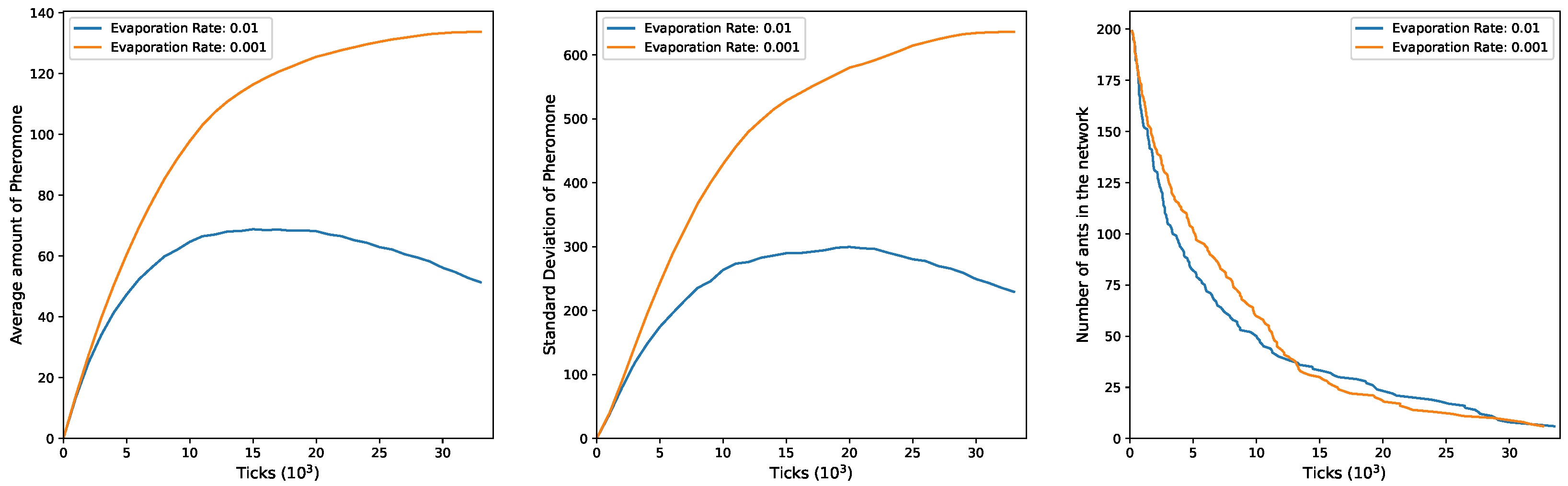
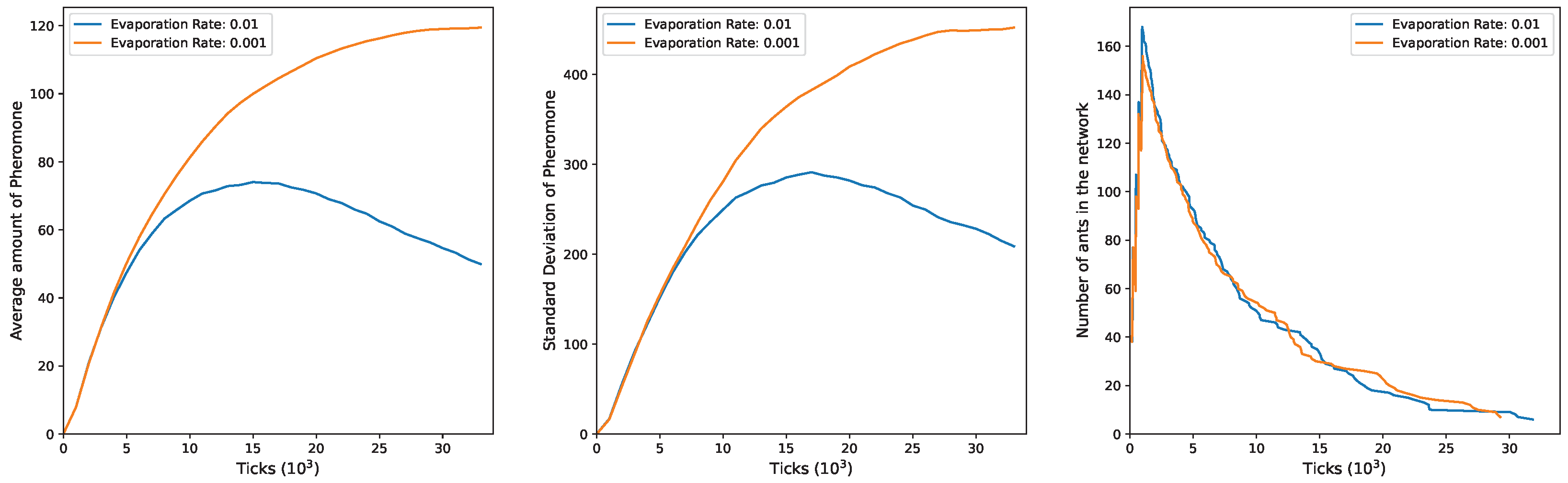
In Figure 3, the outcomes for $g=1$ and $n_g=200$ are illustrated. In the initial phase of the simulation, there is an increase in the mean of pheromones, coinciding with active exploration by a substantial number of ants in the environment. Subsequently, a decline occurs, more pronounced, with an evaporation rate of $0.01$ and a slower stabilization at $0.001$. This pattern underscores the deep connection between mean pheromone levels and the presence of ants in the network. As ants exit the network, there is a corresponding decrease in the pheromone quantity on edges, particularly clear at a higher evaporation rate. This decrease is attributed to the reduced ability of the remaining ants to counteract the ongoing pheromone evaporation. The second plot mirrors these dynamics, illustrating changes in the standard deviation. Also, in this scenario there is an initial rise in the value during the simulation’s early phase, signifying an increase in the heterogeneity of pheromones as ants release them at the edges. As the ants gradually exit the network, the standard deviation decreases when $\rho =0.01$ and stabilizes when $\rho =0.001$. This is consistent with the idea that a smaller ant population in the network results in a diminished ability to counteract the evaporation rate, ultimately leading to a more uniform distribution of pheromone levels across the edges. The third plot depicts the evolving number of ants in the network over time, starting at 200, corresponding to the initial exploration group in the $g=1$ configuration. As time progresses, ants exit with varied trends influenced by the $\rho$ value. Notably, these trends undergo an inversion around $14,000$ ticks.

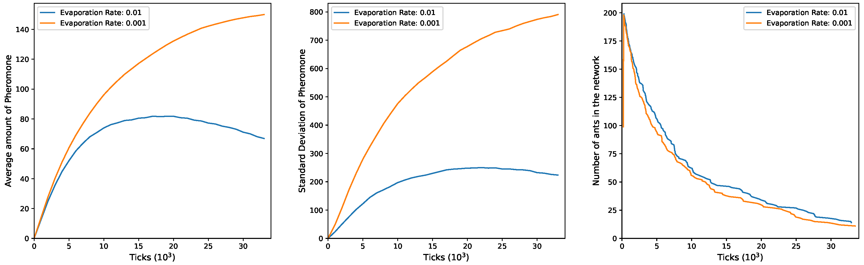
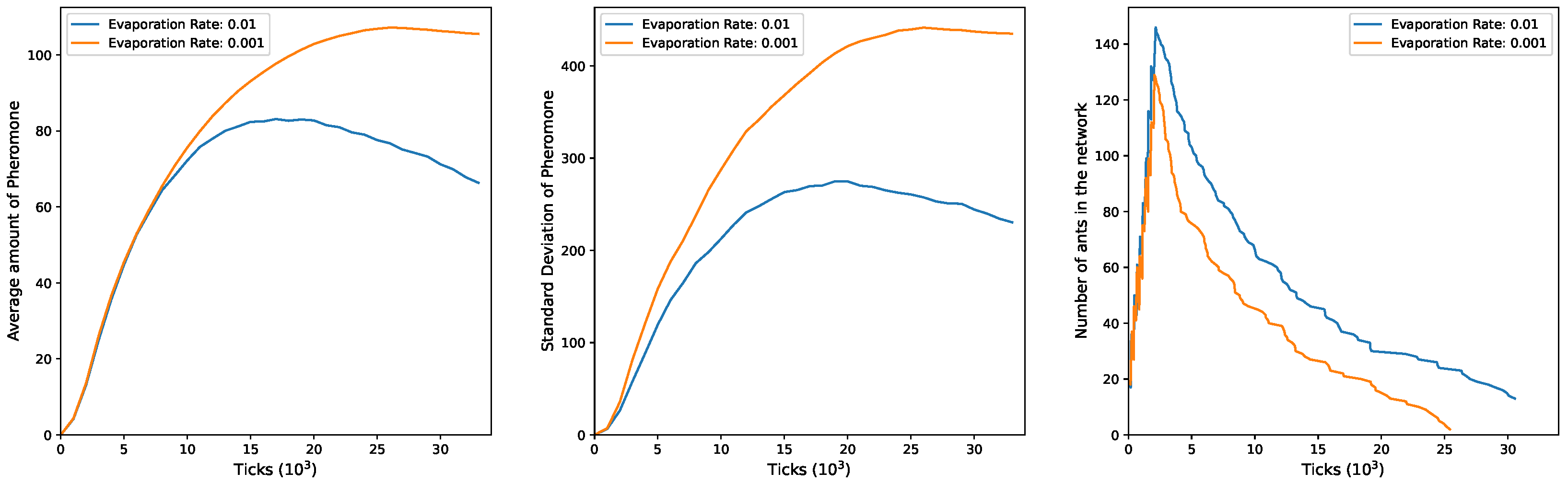
In Figure 4, the plots for $g=2$ and $n_g=100$ exhibit a trend similar to the previous configuration. Both mean pheromones and standard deviation show an initial increase during the simulation. Subsequently, a decline is observed, but only when $\rho =0.01$. Under $\rho =0.001$, both mean and standard deviation continue to rise over time. This discrepancy can be attributed to the more efficient exploratory activity of ants in this setup, resulting in fewer ants being present in the network at any given moment to counteract ongoing pheromone evaporation, particularly with the higher evaporation rate of $\rho =0.01$. The third plot illustrates the evolving number of ants in the network over time, starting at 100 and peaking at 200, indicating the entry of groups 1 and 2. As time progresses, ants exit more rapidly under $\rho =0.001$ and slower under $\rho =0.01$.

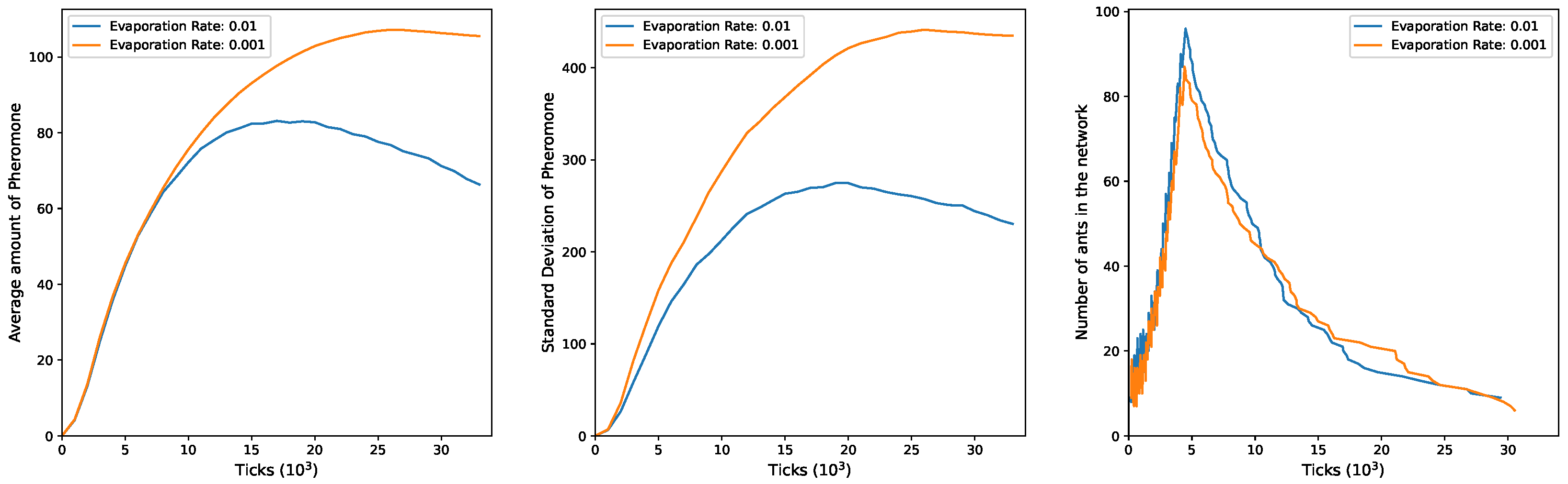
The plots for $g=5$ and $n_g=40$ in Figure 5 follow a similar trend. Both the mean and the standard deviation exhibit an initial increase during the simulation, followed by a decline, but only when $\rho =0.01$. Under $\rho =0.001$, both metrics reach stabilization. As ants gradually exit the environment, their ability to counteract pheromone evaporation is more effective with a low evaporation rate ($\rho =0.001$), resulting in a higher degree of pheromone heterogeneity. Conversely, when the evaporation rate is higher ($\rho =0.01$), the remaining ants in the network struggle to counteract pheromone evaporation, leading to a decrease in the mean and heterogeneity. Concerning the number of ants in the environment, it initiates at 40, with the fluctuations in the plot representing the intermittent entry of the five groups. Over time, ants exit at varying rates depending on the value of $\rho$.

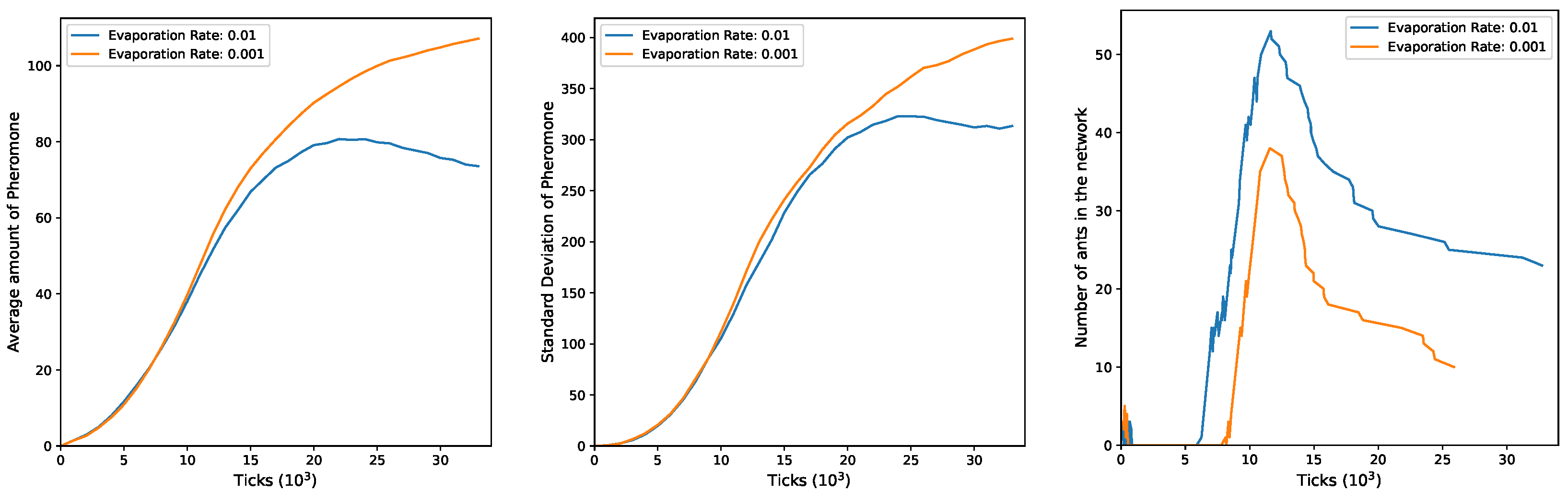
In Figure 6 and Figure 7, the plots for the configurations $g=10$ and $N_g=20$, as well as $g=20$ and $n_g=10$, exhibit a trend similar to previous configurations. For both configurations, both the mean and the standard deviation show an initial increase during the simulation, followed by a decline, but only under $\rho =0.01$. Under $\rho =0.001$, both metrics in both cases reach a stabilization. In other words, as ants gradually exit the environment their ability to counteract pheromone evaporation is more effective with a low evaporation rate ($\rho =0.001$), resulting in a prolonged period of higher pheromone heterogeneity. Conversely, when the evaporation rate is higher ($\rho =0.01$) the remaining ants in the network struggle to counteract pheromone evaporation, leading to a decrease in mean and standard deviation. Regarding the number of ants in the environment, they initiate at 20 and 10, respectively, with the fluctuations in the plot representing the intermittent entry of the other groups (10 and 20, respectively). For $g=10$, it is clear that over time ants exit more rapidly when $\rho =0.01$ than when $\rho =0.001$, suggesting that the ants increasingly benefit from the remaining pheromones on the edges as time unfolds. In contrast, for $g=20$ this pattern holds true but only until around 11,000 ticks, beyond which the two trends reverse.

In Figure 8, for the configuration $g=50$ and $n_g=4$, both the mean and standard deviation show a continuous increase during the simulation when $\rho =0.001$. However, with $\rho =0.01$, the trend in the standard deviation, after an initial phase of increase, starts to decrease, followed by stabilization and a slight subsequent increase. This is in contrast to the mean, which experiences a more pronounced decrease. Furthermore, in this configuration a high degree of heterogeneity is sustained for a more extended period. These behaviors are closely linked to the evolving number of ants in the network, as observed in the third plot. Initially (for $0<T<5000$), groups of four ants engage in exploration, swiftly exiting with no noticeable peaks in the curve. Concurrently, other groups are launched, but their rapid exit is not reflected in the curve. In the subsequent time interval ($5000<T<$ 10,000), there is an increase in the number of ants, marked by fluctuations in the curves. Notably, higher values are observed under $\rho =0.01$, while lower values are seen at $\rho =0.001$. Around 11,000 ticks, the number of ants gradually starts to decrease.

4. Discussion

The observed trends across the two metrics in the overall analysis are deeply connected to the interplay between the number of groups and the evaporation rate. In terms of success rate, the dynamics shift at different evaporation rates. At a higher rate ($\rho =0.01$) the optimal performance is achieved with 10 groups, suggesting that a more consolidated effort among a moderate number of groups is favored for efficient exploration. Conversely, at a lower evaporation rate ($\rho =0.001$) the extended lifespan of pheromones promotes sustained collaboration across 20 groups, leading to improved overall efficiency. The trend in path cost reflects a delicate balance between the collaboration benefits and potential drawbacks of increased group size. At a higher evaporation rate ($\rho =0.01$) the optimal path cost is achieved with 10 groups, denoting an optimal level of cooperation. Conversely, at a lower evaporation rate ($\rho =0.001$), sustained collaboration across 20 groups becomes beneficial due to the extended period of information retention. The slower evaporation rate facilitates distributed collaboration, enhancing exploration efficiency and reducing overall path costs. In this scenario, the persistence of pheromones enables distributed ant groups to communicate better and share information.

In the group analysis, operating as a single group, the colony displayed a remarkable level of consistency, showing comparable success rates and costs at different evaporation rates ($\rho$ values). This consistency suggests that the collective behavior of the colony is inherently robust, adapting seamlessly to varying environmental conditions. Upon division into two groups, a clear dynamic emerged. Group 1 outperformed group 2 when the evaporation rate was higher and vice versa. However, the colony showed an overall consistent performance, hinting at the robustness of its collective decision-making processes. Expanding the analysis to five groups revealed a standout performance by group 1, achieving the highest success rate along with a competitive cost. However, the subsequent groups exhibited signs of performance degradation, highlighting the complexity of managing larger ant colonies with diverse group compositions. Similar trends persisted when the colony was divided into ten groups, with specific groups distinguishing themselves in terms of success rates and costs. Notably, there was a discernible trend of performance degradation progress through the groups. This suggests that as the number of groups increases, the coordination challenges become more pronounced, potentially affecting the overall effectiveness of the colony. Further dividing the colony into twenty and fifty groups exposed a more intricate landscape of performance variations. While certain groups consistently excelled, demonstrating high success rates and cost-effectiveness, others displayed a noticeable decline in performance. Overall, it is noteworthy that the optimization process does not reach its best with the final group of ants in each configuration. In other words, the group achieving the optimal values in terms of success rate or path cost is typically one of the initial groups. Subsequent groups tend to exhibit a decline in performance after one of these early groups attains optimal values in both evaluation metrics.

Finally, in the pheromone distribution analysis, in general, the plots across all configurations exhibit comparable trends. Initially, there is a noticeable increase in mean pheromone levels, corresponding to active exploration and a significant presence of ants. However, a subsequent decline becomes apparent, particularly significant when there is a higher evaporation rate ($\rho =0.01$). This decrease can be attributed to the reduced capacity of the remaining ants to counteract the ongoing evaporation of pheromones. In contrast, lower evaporation rates ($\rho =0.001$) result in more extended periods of elevated pheromone levels. The standard deviation mirrors this pattern, suggesting heightened heterogeneity during exploration and a more uniform distribution as ants exit. The number of ants in the network undergoes fluctuations over time, reaching a peak corresponding to the entry of the last group into the environment. As various groups enter and exit, the network experiences dynamic changes. Generally, a lower evaporation rate leads to a swifter and more efficient exit of ants from the network. These findings shed light on why, in group analysis, the groups that perform exceptionally well are typically among the first rather than the last in each configuration. What emerges is that once a particular group within the considered configuration discovers or achieves the optimal value in terms of success rate and cost, subsequent groups exhibit a decline in their performance. This phenomenon could be attributed to the non-constant presence of groups and ants within the environment over time. Groups initiate exploration at regular intervals, but as time progresses ants exit the environment. Consequently, the activity of pheromone evaporation becomes increasingly significant because the remaining ants within the environment struggle to counteract this process. Consequently, there is yet again an increase in the homogeneity of pheromone distribution across the edges. As a result, each path becomes similar for the ants, impeding their ability to optimize path choices.

5. Conclusions

This paper introduces an agent-based model based on the ACO paradigm where ants are memory-enhanced to explore how partitioning a colony into groups influences the algorithm’s performance. The study specifically delves into the roles of group size and number in the context of a network analysis. Within the model, a collective of ants, starting from a specified location, collaboratively works to find the optimal path leading to the exit within a grid network. The overarching objectives of the colony include maximizing the number of ants successfully leaving and minimizing path costs. Three different kinds of analysis were conducted: an overall analysis, to analyze the performance of the whole colony concerning the two evaluation metrics when divided into groups of different sizes; a group analysis, to investigate the performance of each group into which the colony is partitioned; and a pheromone distributions analysis, to discern any correlation between the temporal distribution of pheromones on the edges and the number of ants navigating the network during the simulation.

In the overall analysis, a nuanced relationship emerged between the number of groups and the algorithm’s performance. At a higher evaporation rate, the optimal configuration involved 10 groups, obtaining the best success rate and path costs. It follows that under conditions of accelerated pheromone decay a moderate level of colony partitioning enhances effective collaboration. Conversely, at a lower evaporation rate, a superior performance was observed with 20 groups, emphasizing the role of prolonged pheromone lifespan in facilitating distributed collaboration and reducing overall costs. This finding underscores the significance of pheromone persistence, particularly in scenarios where environmental conditions permit longer-lasting pheromones.

The group analysis delved deeper into the performance of individual groups. Notably, the colony operating as a single group demonstrated consistent adaptability across different evaporation rates. However, as the number of groups increased, a complex landscape of performance rates emerged. Optimal values in success rate or path cost were typically achieved by one of the initial groups, with subsequent groups showing a decline in performance. This highlights the coordination challenges that escalate with the number of groups and their interactions, emphasizing the need for careful consideration in partitioning colonies, especially in larger-scale scenarios, to mitigate challenges associated with managing diverse groups effectively.

The pheromone distribution analysis provided additional insights into the correlation between pheromone dynamics, ant presence, and group behavior. As the number of ants increased, mean pheromone levels collectively rose, indicating active exploration. However, a subsequent decline, particularly noticeable at higher evaporation rates, emphasized the challenge of sustaining the pheromone quantity over time. The standard deviation analysis added depth to this understanding, revealing that a more uniform distribution, as indicated by lower values, could make it harder for ants to differentiate paths and exit efficiently. Conversely, higher standard deviation values suggested greater heterogeneity, enabling ants to effectively use pheromone signals for their exploration. The temporal dynamics of group entry and exit further highlighted the transient nature of group presence. Peaks in mean pheromone levels aligned with group entry, followed by decreases indicating exits. This temporal pattern underscores the dynamic nature of group interactions and their impact on pheromone distribution.

In summary, our study reveals a correlation between the partitioning of ant colonies and the quality of solutions within an ACO framework, shedding light on the complex interplay between individual ant behaviors and collective dynamics. The adaptability of ant colonies, discerned through the optimal degree of partitioning influenced by pheromone lifespan and group entry into the environment, underscores their responsiveness to diverse environmental conditions. The importance of the evaporation rate of pheromones emerges as a key factor in comprehending group dynamics during maze navigation. When pheromones persist for a longer time, dividing the colony into more groups becomes advantageous. This is because it allows for a more distributed and efficient exploration of the maze. The surplus of pheromones in the network, if not properly managed, could hinder exploration by leading ants in unproductive directions. Conversely, the heightened performance of initial groups highlights the critical role of the early exploration stages. The delicate balance between pheromone presence and evaporation rate fosters effective communication, enabling these groups to efficiently identify and reinforce optimal paths. Yet, as the simulation progresses and ants exit the network, subsequent groups experience performance declines due to a diminished ability to counteract pheromone evaporation. The observed variability in optimal configurations underscores the need for adaptive strategies to optimize ACO performance in evolving environmental conditions. The demonstrated adaptability of the Memory-Enhanced Ant Colony Optimization (ME-ACO) framework holds practical implications, particularly in fields such as logistics, supply chain management, and energy distribution. Dynamically adjusting group configurations could optimize transportation routes in response to changing traffic conditions and seasonal demands. Similarly, in smart grids and energy management, adaptability could enhance efficiency by responding to fluctuating demands and renewable energy availability. Expanding beyond optimization, the ME-ACO framework can be used in modeling and understanding collective behaviors in diverse scenarios. Its flexibility might be crucial in capturing the complex and dynamic interactions among social agents as they interact with the environment and each other. Utilizing an indirect communication mechanism, these interactions give rise to the emergence of collective behaviors, providing a valuable perspective on social dynamics across various contexts. Future extensions of the presented framework may include a sensitivity analysis of parameters to explore model dynamics under different configurations, additional experiments with more complex environments, possibly incorporating benchmark networks from the literature, and the consideration of a dynamic version of the framework where group number and size adapt dynamically to environmental conditions.