Improved Load Frequency Control in Power Systems Hosting Wind Turbines by an Augmented Fractional Order PID Controller Optimized by the Powerful Owl Search Algorithm

Abstract

The penetration of intermittent wind turbines in power systems imposes challenges to frequency stability. In this light, a new control method is presented in this paper by proposing a modified fractional order proportional integral derivative (FOPID) controller. This method focuses on the coordinated control of the load-frequency control (LFC) and superconducting magnetic energy storage (SMES) using a cascaded FOPD–FOPID controller. To improve the performance of the FOPD–FOPID controller, the developed owl search algorithm (DOSA) is used to optimize its parameters. The proposed control method is compared with several other methods, including LFC and SMES based on the robust controller, LFC and SMES based on the Moth swarm algorithm (MSA)–PID controller, LFC based on the MSA–PID controller with SMES, and LFC based on the MSA–PID controller without SMES in four scenarios. The results demonstrate the superior performance of the proposed method compared to the other mentioned methods. The proposed method is robust against load disturbances, disturbances caused by wind turbines, and system parameter uncertainties. The method suggested is characterized by its resilience in addressing the challenges posed by load disturbances, disruptions arising from wind turbines, and uncertainties surrounding system parameters.

1. Introduction

The use of wind turbines in power systems is growing due to the increasing demand for sustainable and environmentally friendly electrical energy [1,2,3]. Wind turbines have several advantages as a stable source of electricity in power systems, such as: (1) abundant energy source: for electricity generation, wind turbines require an abundant wind energy source that is usually available day and night; (2) reduced environmental pollution: using wind turbines as a clean energy source reduces environmental pollution; (3) cost reduction in electricity production: the cost of electricity production with wind turbines is lower than that of fossil fuels. Despite these advantages, wind turbines in power systems have some drawbacks, including the complexity of load-frequency control (LFC) [4,5,6]. Wind turbines rely on wind, which is naturally fluctuating and can complicate LFC in power systems [7]. In power systems, a balance is maintained between generation and consumption [8]. Should any disturbance arise, impeding the smooth functioning of this intricate network, the primary control loop immediately intervenes to restrict any deviations in frequency [9]. Yet it is the secondary control loop, known as the LFC system, which assumes responsibility for restoring frequency to their nominal levels [10]. In an earnest endeavor to enhance frequency stability within the power system, various controllers have been proposed for LFC systems [11,12,13,14,15,16,17,18,19,20,21,22,23,24,25,26,27,28,29,30,31,32,33,34,35,36,37,38,39,40,41,42,43,44,45].

The classic proportional integral derivative (PID) controller is still one of the most popular and widely used controllers in the power industry, which is widely used in power system LFC due to its simplicity, ease of use, fast performance, and stability [11,12,13,14,15,16,17,18,19,20,21,22,23,24,25]. In LFC systems related to power systems, a number of PID controllers are used in order to improve frequency stability; among these PID controllers [11,12] are: PID controllers whose parameters are optimized using the ICA [13] (see list of abbreviations at the end of the article), PID controllers whose parameters are optimized using the PSO [14], PID controllers whose parameters are optimized using the EHO [15], PID controllers whose parameters are optimized using the ACO [16], fuzzy PID controllers [17], fuzzy PID controllers whose parameters are optimized using the optimization algorithm based on novel HLUS-TLBO [18], fuzzy PID controllers whose parameters are optimized using the DE algorithm [19], fuzzy PID controllers whose parameters are optimized using the HDE-PS algorithm [20], fuzzy PID controllers whose parameters are optimized using the PSO [21], fuzzy PID controllers whose parameters are optimized using ACO [22], fuzzy PID controllers whose parameters are optimized using the HFA-PS algorithm [23], control fuzzy PID controllers whose parameters are optimized using MBA [24], and fuzzy PID controllers whose parameters are optimized using FA [25]. In [26], the fuzzy PID controller whose coefficients are optimized using GA is used to improve the frequency of the power system. The PID controller does not perform effectively against disturbances in the power system and the uncertainty of the parameters related to the power system. Fuzzy PID controllers are somewhat resistant to power system disturbances, but they do not perform well against the uncertainty related to the power system.

The fractional order PID (FOPID) controller has two degrees of freedom compared to the PID controller, and these two degrees of freedom have advantages such as: (1) more accuracy, (2) better stability, and (3) robust performance in systems with disturbance and parameter uncertainty [27]. Due to these advantages, FOPID controllers have been widely used in LFC systems related to the power system in order to improve the frequency stability; among these FOPID controllers [28,29] are: FOPID controllers whose parameters are optimized using the ICA [30], FOPID controllers whose parameters are optimized using the GBMO [31], FOPID controllers whose parameters are optimized using the SCA [32], FOPID controllers whose parameters are optimized using the PSO [33], and FOPID controllers whose parameters are optimized using the JSO algorithm [34]. The performance of FOPID controllers is favorable against disturbances and uncertainty related to system parameters, but their performance is affected by severe disturbances.

Superconducting magnetic energy storage (SMES) systems store electric energy in their magnetic field and release it as needed, making them a significant contributor to improving frequency stability alongside the LFC system in power systems [35], due to their extended lifespan and high storage capacity. In [36], coordinated control of the LFC system and SMES is discussed using an H2/H∞ robust controller. However, designing such a robust controller necessitates an accurate model of the power system, and since some components may be ignored in the model, the controller’s optimal performance may be compromised in real-world systems. Another approach to coordinated control is presented in [37], where a neuro-fuzzy controller is employed. Although the neuro-fuzzy controller demonstrates good results in addressing uncertainties related to the power system parameters, it is not robust against disturbances caused by the power system load.

In [38], the coordinated control of the LFC system and SMES using a type-2 fuzzy controller is discussed. However, this controller is also not resistant to severe disturbances in the power system. Similarly, [39] explores the coordinated control of the LFC system and SMES using a PID controller with parameters optimized by the DE algorithm. Unfortunately, this method is also not resistant to disturbances and uncertainties in power system parameters. Reference [40] presents the coordinated control of the LFC system and SMES using a PI controller with parameters optimized using the PSO, taking into account the presence of wind turbines in the power system. However, the performance of this control method is challenging due to the severe disturbances caused by the wind turbine, making the PI controller optimized with the PSO non-resistant to such disturbances. Reference [41] discusses the coordinated control of the LFC system and SMES using a PID controller with parameters optimized by the MSA, considering the presence of wind turbines in the power system. Nevertheless, the performance of this control method is not resistant to load disturbances and disturbances from the wind turbine. In [42], the coordinated control of the LFC system and SMES using a dynamic resistance controller in the presence of wind turbines is discussed. This method exhibits resistance to load disturbances, wind turbine disturbances, and uncertainties related to power system parameters. However, it has certain drawbacks, including: (1) the complexity of the control method, which requires setting numerous parameters and involves heavy calculations, and (2) the necessity for an accurate power system model, as some parameters cannot be accurately modeled, impacting the performance of this control method.

Currently, cascaded controllers are recognized for their superior system control performance compared to single controllers such as PID and FOPID. These cascaded controllers have been employed to enhance frequency stability in power systems [43,44,45,46]. In [43], a cascaded FOPI–FOPD controller with optimized parameters using the DSA method is utilized to improve frequency stability in the power system. The FOPI–FOPD controller parameters are set using the ITAE cost function, and the simulation time is set to 10 s. In [44], a PI–TID cascaded controller is introduced, and its parameters are adjusted using the CBO algorithm to enhance frequency stability in the power system. The PI–TID cascaded controller parameters are determined using the ISE cost function, and the simulation time is set to 120 s. Furthermore, in [45], a PI–FOPID cascaded controller is investigated for improving frequency stability in the power system. The parameters of the PI–FOPID cascaded controller are adjusted using the GTO technique. The ITAE cost function is employed to set the PI–FOPID cascaded controller parameters, and the simulation time is set to 30 s. In [46], the cascaded FOPDN–FOPIDN controller, whose coefficients are optimized using the CSA, is utilized for automatic generation control of production in the power system. The ISE cost function is considered in optimizing the controller coefficients, and the simulation time is set to 100 s.

The main difference between the ISE and ITAE cost functions lies in the method of error calculation. Both cost functions are used to evaluate the quality of control, but they differ in how they quantify and integrate the errors over time. In the ISE cost function, the squared errors at each time point are integrated over the entire time period. This means that the errors are squared and then summed up. The ISE cost function is commonly used for stable control of control systems. On the other hand, the ITAE cost function calculates the absolute errors at each time point, multiplies them by time, and then sums them up. The ITAE cost function captures the process dynamics in the time domain. It emphasizes the errors that occur during the initial response of the system and can be more sensitive to transient behavior. In the context of the paper mentioned, the ISE cost function is used to evaluate the frequency stability of the power system in the presence of a wind turbine. The goal is to control the power system effectively. Reference [41] also utilizes the ISE cost function to control the frequency of the power system with a wind turbine and to adjust the coefficients of the PID controller. The choice of the ISE cost function in this paper allows for comparison with the results obtained using the PID controller in [41].

In this paper, a novel method called the FOPD–FOPID cascaded controller is proposed for the coordinated control of the LFC system and SMES in a power system that includes a wind turbine. The parameters of the FOPD–FOPID cascaded controller are optimized using the developed Owl Search Algorithm (DOSA). The reason for selecting the FOPD–FOPID cascaded controller over other cascaded controllers, such as PI–FOPID, in the power system structure is that the FOPD–FOPID controller, incorporating the FOPD component, provides more accurate and rapid response to frequency changes in the presence of a wind turbine. This characteristic enhances the frequency stability of the power system and ensures robustness against load disturbances, wind turbine disturbances, and uncertainties associated with power system parameters. The DOSA algorithm is employed to optimize the parameters of the cascaded controller within the power system structure. The DOSA algorithm offers several advantages over other meta-heuristic algorithms such as ABC, PSO, MSA, and GTO. These advantages include: (1) robustness in the face of uncertainty related to the objective function, (2) a reduced number of control parameters, and (3) global optimization capability. The paper presents several key innovations, including:

(1)

Enhancing the responsiveness of the power system in the presence of a wind turbine using the cascaded FOPD–FOPID controller.

(2)

Refining the parameters of the FOPD–FOPID controller through the application of the novel DOSA approach, which has not been previously explored in power system research.

(3)

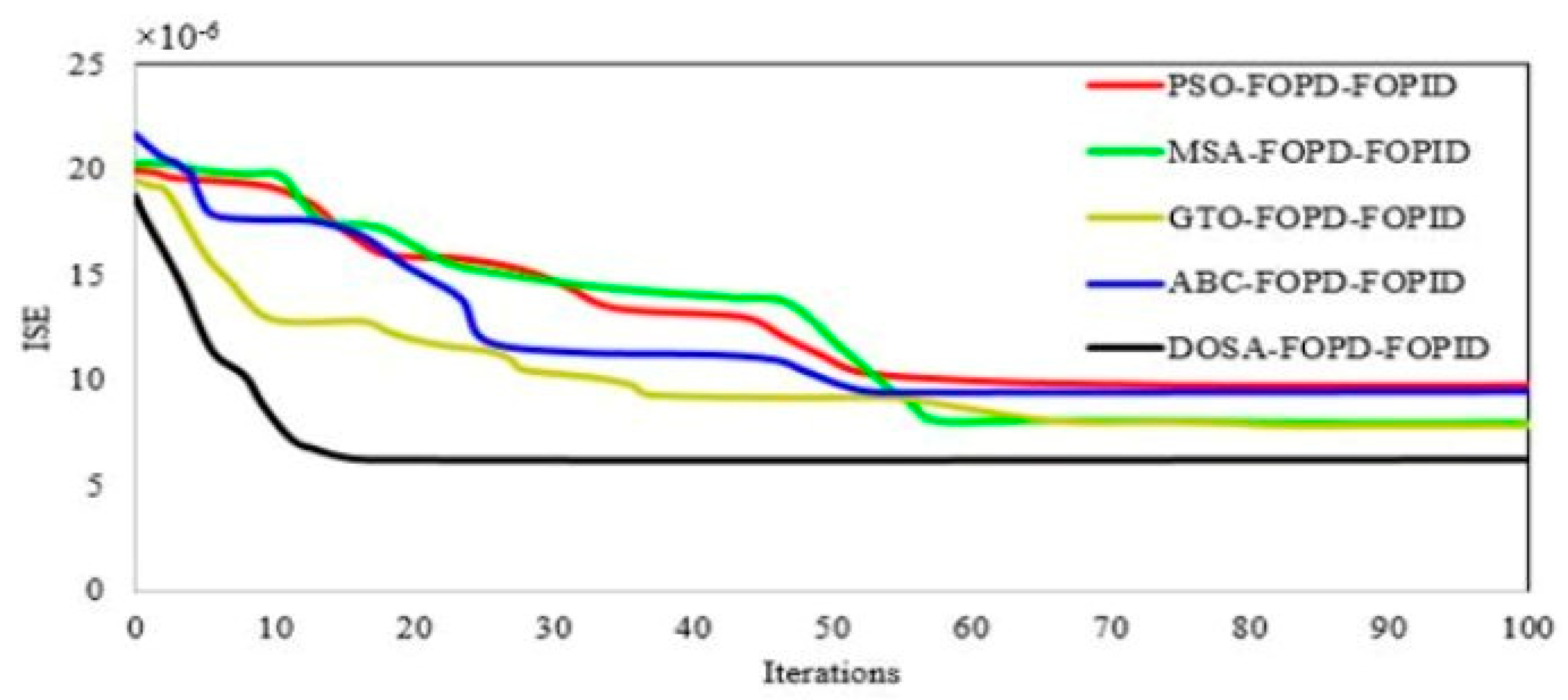
Evaluating and comparing the effectiveness of the proposed algorithm with GTO, MSA, PSO, and ABC algorithms for optimizing the parameters of the FOPD–FOPID controller, employing an objective function based on ISE.

(4)

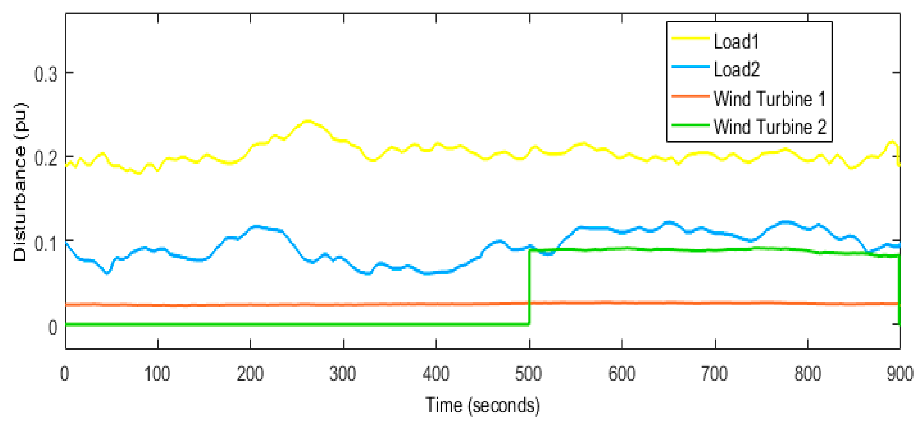
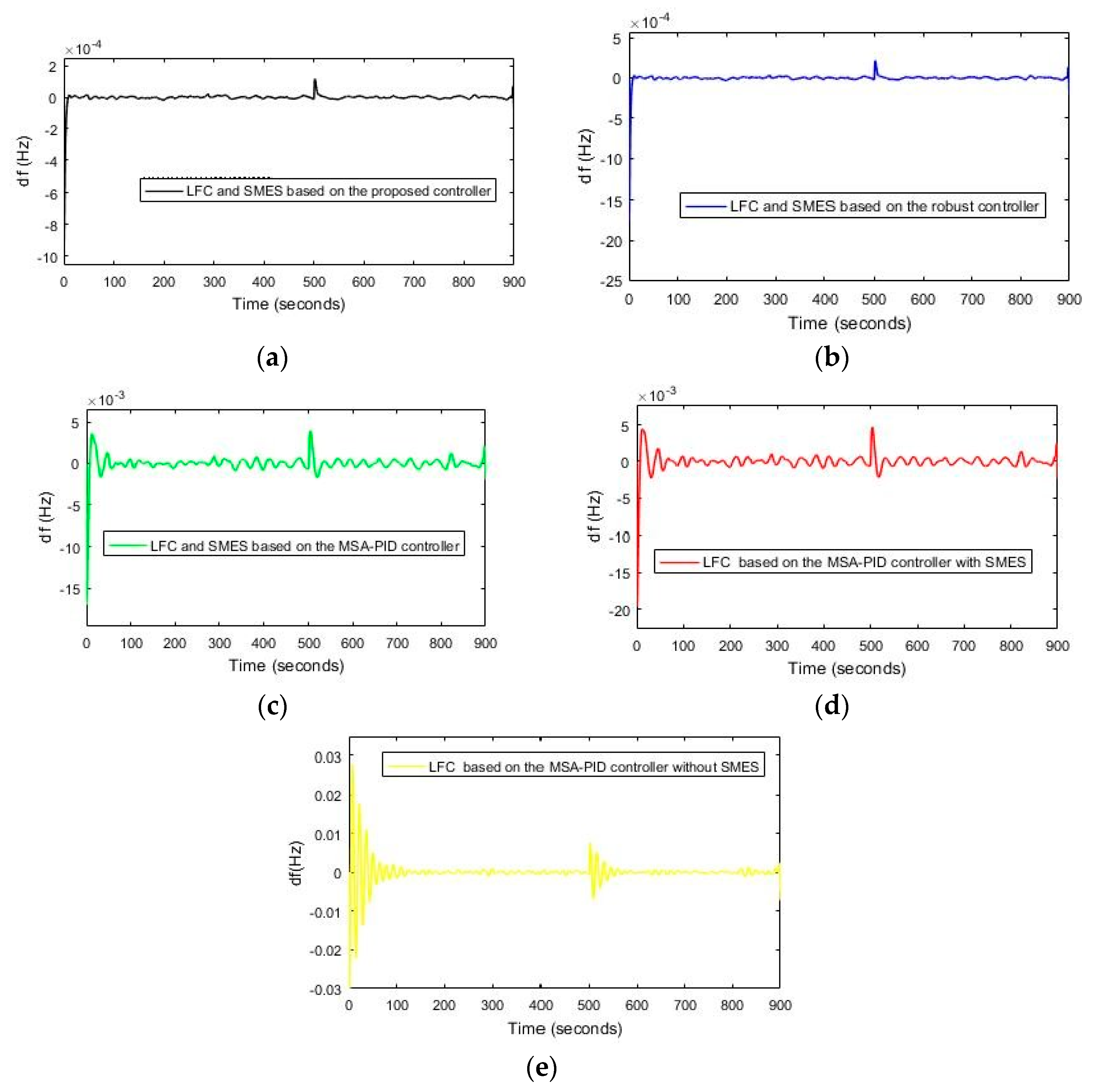
Conducting a comprehensive assessment of the performance of the DOSA–FOPD-FOPID controller for improving coordinated control capabilities within both the LFC system and SMES, considering disturbances and uncertain power system variables.

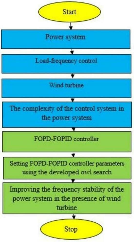
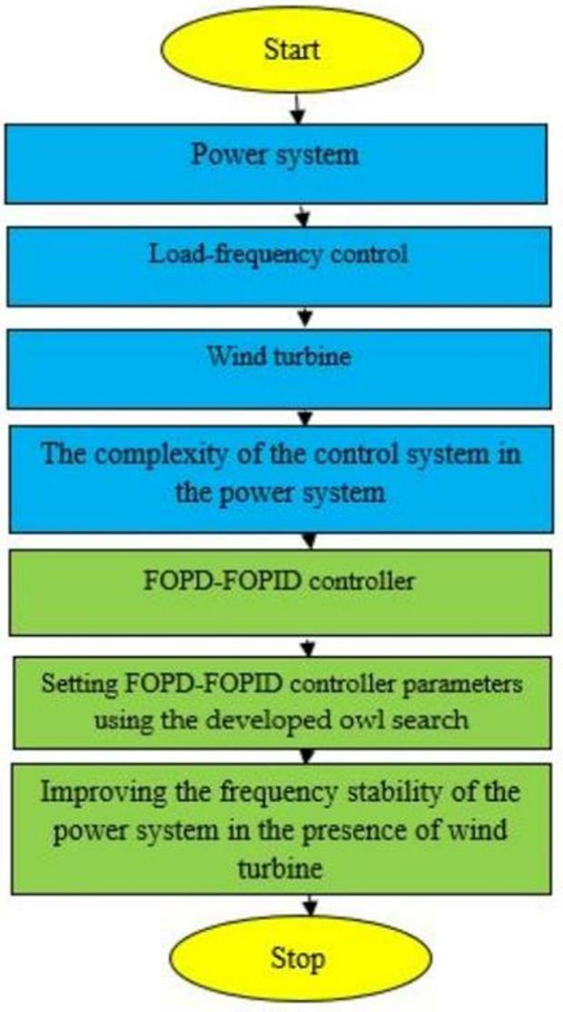
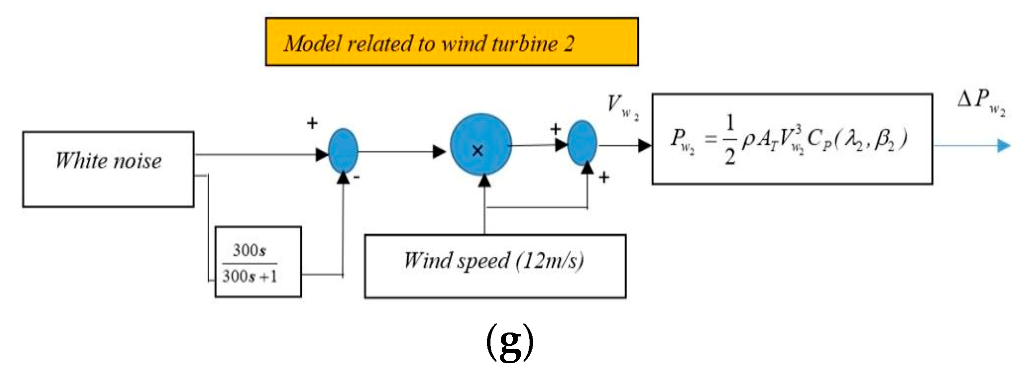
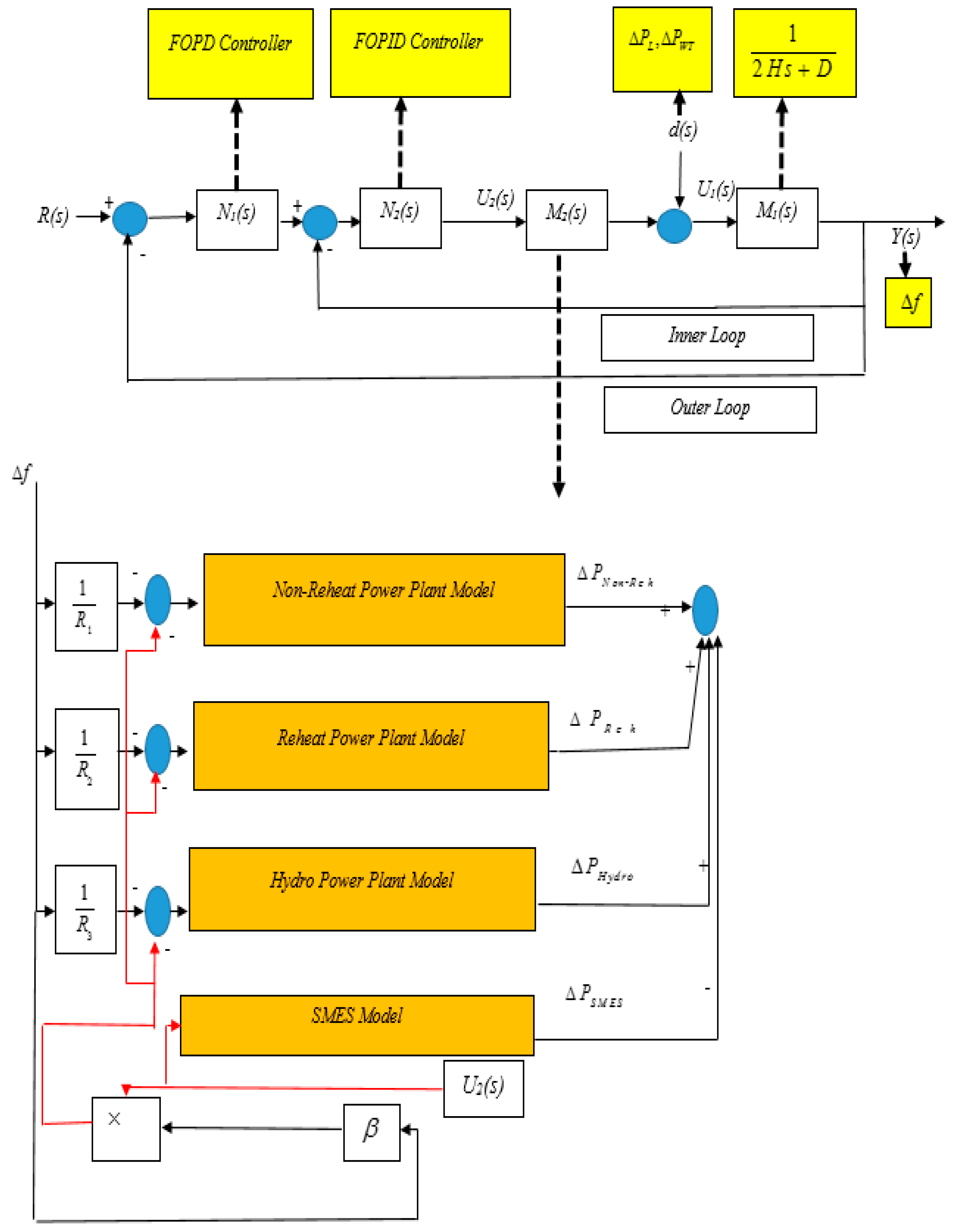
2. The Power System under Scrutiny

In this section, the structure of the power system under scrutiny and the state–space equations of the power system under scrutiny are discussed.

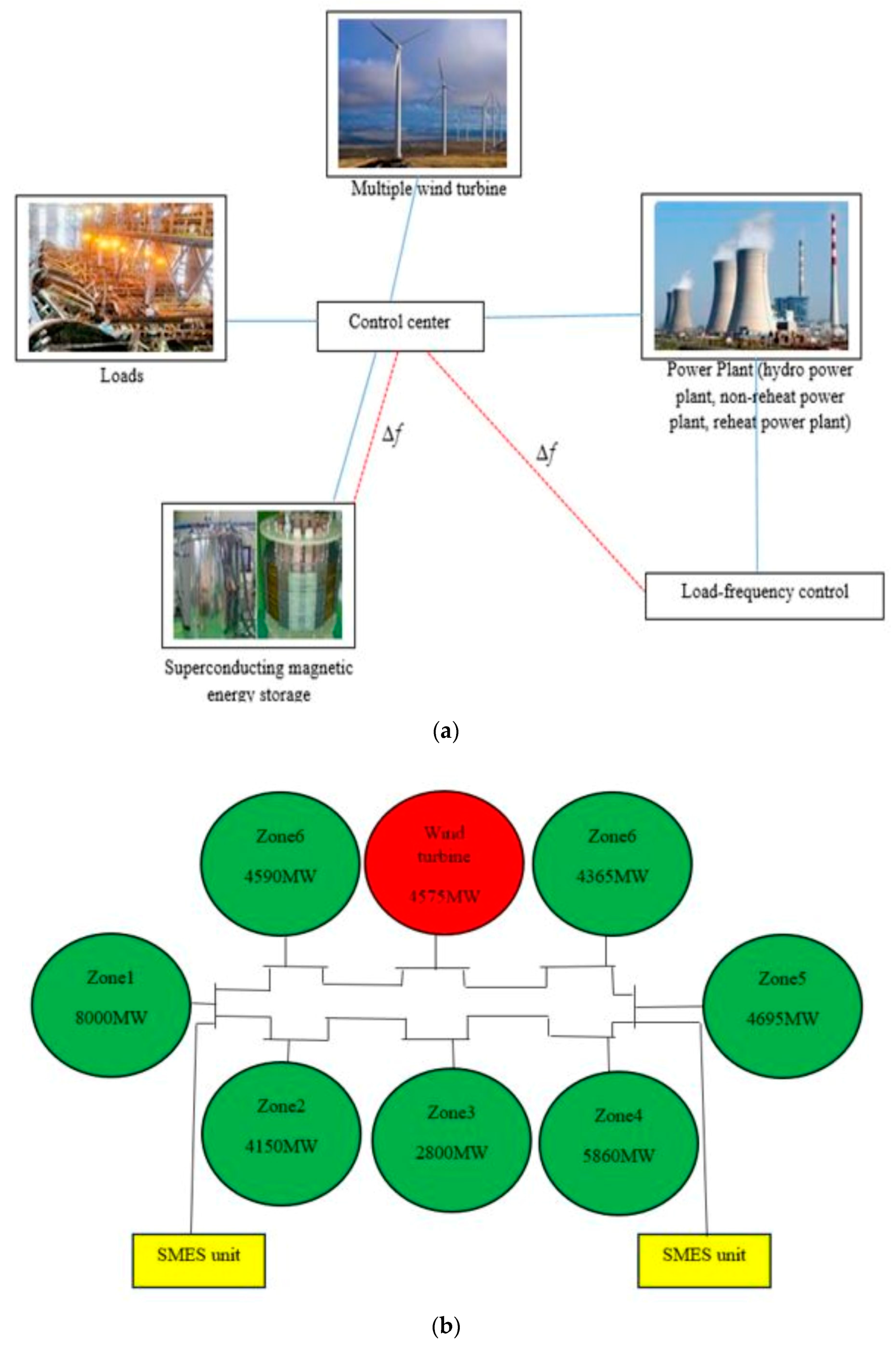
2.1. The Structure of the Power System under Scrutiny

Figure 1a shows the power system configuration incorporating a wind turbine, as described in references [5,42]. Figure 1b shows a single-line diagram of the studied power system [40,41,42]. This system comprises a hydro power plant, non-reheat power plants, reheat power plants, multiple wind turbines, SMES, and a load [40,41,42]. The total power generated by the system is 38,000 MW, while the peak load amounts to 29,000 MW [40,41,42]. Figure 2 illustrates the dynamic model of the power system, taking into account the presence of the wind turbine. The model utilized in this context is a reduced-order (first-order) model, which proves advantageous for analyzing the frequency stability of the power system. The wind turbine model, as shown in Figure 2, is comprehensively described in [40,41,42]. Figure 2 illustrates the model of the turbine for frequency control [40,41,42]. In this model, the wind speed is multiplied by a random speed fluctuation, which is derived from the white noise block in MATLAB/SIMULINK. This multiplication allows for the estimation of random fluctuations in the wind output power. Based on Figure 2, the power system incorporates a coordinated control scheme consisting of an FOPD-FOPID cascaded controller. This controller’s parameters are optimized using the DOSA method, aiming to enhance the frequency stability of the power system in the presence of a wind turbine. The wind turbine exhibits oscillatory behavior and is influenced by the wind speed. The inclusion of the production rate limit definition has led to an improved accuracy in the dynamic model employed for the power system [40,41,42]. The production rate limits are set at 0.2 pu MW/min for non-reheat power plants, 0.1 pu MW/min for reheat power plants, and 0.5 pu MW/min for the hydro power plant [40,41,42].

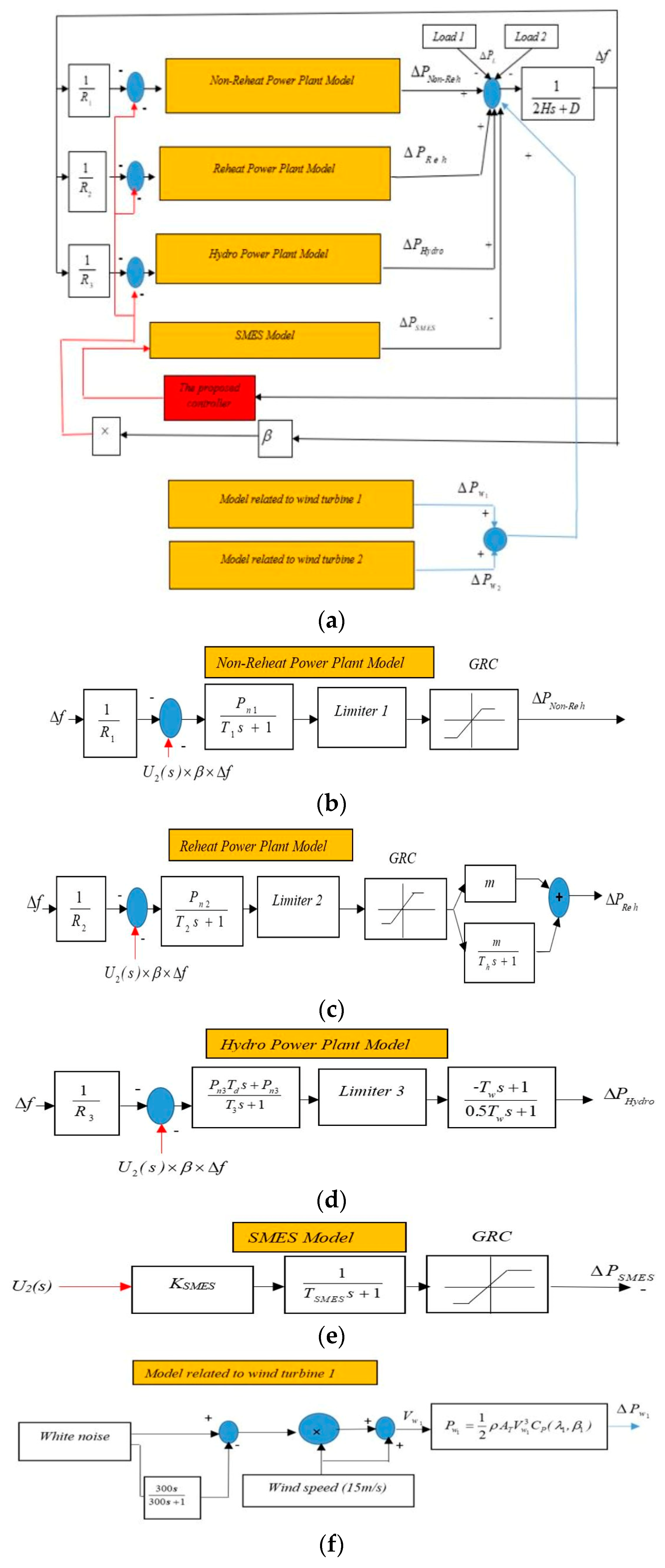
2.2. The State–Space Equations of the Power System under Scrutiny

The design of the proposed controller for the coordinated control of the LFC system and SMES involves the utilization of state-space equations, as illustrated by Equations (1) and (2). The parameters specific to the analyzed power system are provided in

Table 1. Parameters specific to the analyzed power system [40,41,42].

Parameter	Value	Parameter	Value
Pn2	0.6107	R2	2.5
Pw,2	3000 KW	Pn1	0.2529
Pn3	0.1364	H	5.7096
T3	90	Th	6
T2	0.4	R3	1
T1	0.4	m	0.5
Td	5	β	1
Pw,1	750 KW	D	0.028
Tw	1	R1	2.5
Pw,2	3000 KW

[40,41,42].

$$\begin{array}{l}\left[\begin{array}{l}\stackrel{•}{\Delta f}\\ \stackrel{•}{\Delta P_{Non-\mathrm{Re}h}}\\ \stackrel{•}{\Delta P_{\mathrm{Re}h}}\\ \stackrel{•}{\Delta P_{g2}}\\ \stackrel{•}{\Delta P_{Hydro}}\\ \stackrel{•}{\Delta P_{g3}}\\ \stackrel{•}{\Delta P_{WT}}\\ \stackrel{•}{\Delta P_{SMES}}\end{array}\right]=\frac{2m}{T_h}\left[\begin{array}{llllllll}\frac{-D}{2H}& \frac{1}{2H}& \frac{1}{2H}& 0& \frac{1}{2H}& 0& \frac{1}{2H}& \frac{1}{2H}\\ \frac{-P_{n1}}{T_1{R}_1}& \frac{-1}{T_1}& 0& 0& 0& 0& 0& 0\\ \frac{-m{P}_{n2}}{T_2{R}_2}& 0& \frac{-1}{T_h}& (\frac{2m}{T_h}-\frac{m}{T_2})& 0& 0& 0& 0\\ \frac{-P_{n2}}{T_2{R}_2}& 0& 0& \frac{-1}{T_2}& 0& 0& 0& 0\\ (\frac{-T_d{P}_{n3}D}{T_3{R}_{3}H}+\frac{2P_{n3}}{T_3{R}_3})& (\frac{T_d{P}_{n3}}{T_3{R}_{3}H})& (\frac{T_d{P}_{n3}}{T_3{R}_{3}H})& 0& (\frac{T_d{P}_{n3}}{T_3{R}_{3}H}-\frac{2}{Tw})& (\frac{2}{Tw}+\frac{2}{T3})& 0& 0\\ (\frac{T_d{P}_{n3}D}{2T_3{R}_{3}H}-\frac{P_{n3}}{T_3{R}_3})& (\frac{-T_d{P}_{n3}}{2T_3{R}_{3}H})& (\frac{-T_d{P}_{n3}}{2T_3{R}_{3}H})& 0& (\frac{-T_d{P}_{n3}}{2T_3{R}_{3}H})& \frac{-1}{T_3}& 0& 0\\ \frac{-D_i}{T_{SMES}}& 0& 0& 0& 0& 0& \frac{-1}{T_{WT}}& 0\\ 0& 0& 0& 0& 0& 0& 0& \frac{-1}{T_{SMES}}\end{array}\right]\left[\begin{array}{l}\stackrel{}{\Delta f}\\ \stackrel{}{\Delta P_{Non-\mathrm{Re}h}}\\ \stackrel{}{\Delta P_{\mathrm{Re}h}}\\ \stackrel{}{\Delta P_{g2}}\\ \stackrel{}{\Delta P_{Hydro}}\\ \stackrel{}{\Delta P_{g3}}\\ \stackrel{}{\Delta P_{WT}}\\ \stackrel{}{\Delta P_{SMES}}\end{array}\right]+\left[\begin{array}{l}0\\ \frac{-P_{n1}}{T_1}\\ \frac{-m{P}_{n2}}{T_2}\\ \frac{-P_{n2}}{T_2}\\ \frac{2P_{n3}}{T_3}\\ \frac{-P_{n3}}{T_3}\\ 0\\ \frac{-K_{SMES}}{T_{SMES}}\end{array}\right]\left[u\right]\\ +\left[\begin{array}{cc}0-\hfill & \hfill \frac{1}{2H}\hfill \\ 0\hfill & \hfill 0\hfill \\ 0\hfill & \hfill 0\hfill \\ 0\hfill & \hfill 0\hfill \\ 0\hfill & \hfill \frac{-T_d{P}_{n3}}{T_3{R}_{3}H}\hfill \\ 0\hfill & \hfill \frac{T_d{P}_{n3}}{2T_3{R}_{3}H}\hfill \\ \frac{-1}{T_{WT}}\hfill & \hfill 0\hfill \\ 0\hfill & \hfill 0\hfill \end{array}\right]\left[\begin{array}{l}\Delta P_{wi}\\ \Delta P_L\end{array}\right]\end{array}$$

(1)

$$y=\left[1\hspace{0.17em}\hspace{0.17em}\hspace{0.17em}\hspace{0.17em}\hspace{0.17em}0\hspace{0.17em}\hspace{0.17em}\hspace{0.17em}\hspace{0.17em}\hspace{0.17em}\hspace{0.17em}\hspace{0.17em}0\hspace{0.17em}\hspace{0.17em}\hspace{0.17em}\hspace{0.17em}\hspace{0.17em}\hspace{0.17em}\hspace{0.17em}0\hspace{0.17em}\hspace{0.17em}\hspace{0.17em}\hspace{0.17em}\hspace{0.17em}\hspace{0.17em}\hspace{0.17em}\hspace{0.17em}0\hspace{0.17em}\hspace{0.17em}\hspace{0.17em}\hspace{0.17em}\hspace{0.17em}\hspace{0.17em}\hspace{0.17em}\hspace{0.17em}0\hspace{0.17em}\hspace{0.17em}\hspace{0.17em}\hspace{0.17em}\hspace{0.17em}\hspace{0.17em}0\hspace{0.17em}\hspace{0.17em}\hspace{0.17em}\hspace{0.17em}\hspace{0.17em}\hspace{0.17em}0\right]\left[\begin{array}{l}\stackrel{}{\Delta f}\\ \Delta P_{Non-reh}\\ \Delta P_{\mathrm{Re}h}\\ \Delta P_{g2}\\ \Delta P_{Hydro}\\ \Delta P_{g3}\\ \Delta P_{WT}\\ \Delta P_{SMES}\end{array}\right]$$

(2)

3. Design of the Proposed Controller for the Power System

This section provides an overview of the proposed controller’s structure, FOPID controller, an analysis of the DOSA, and the design process of the proposed controller utilizing the DOSA.

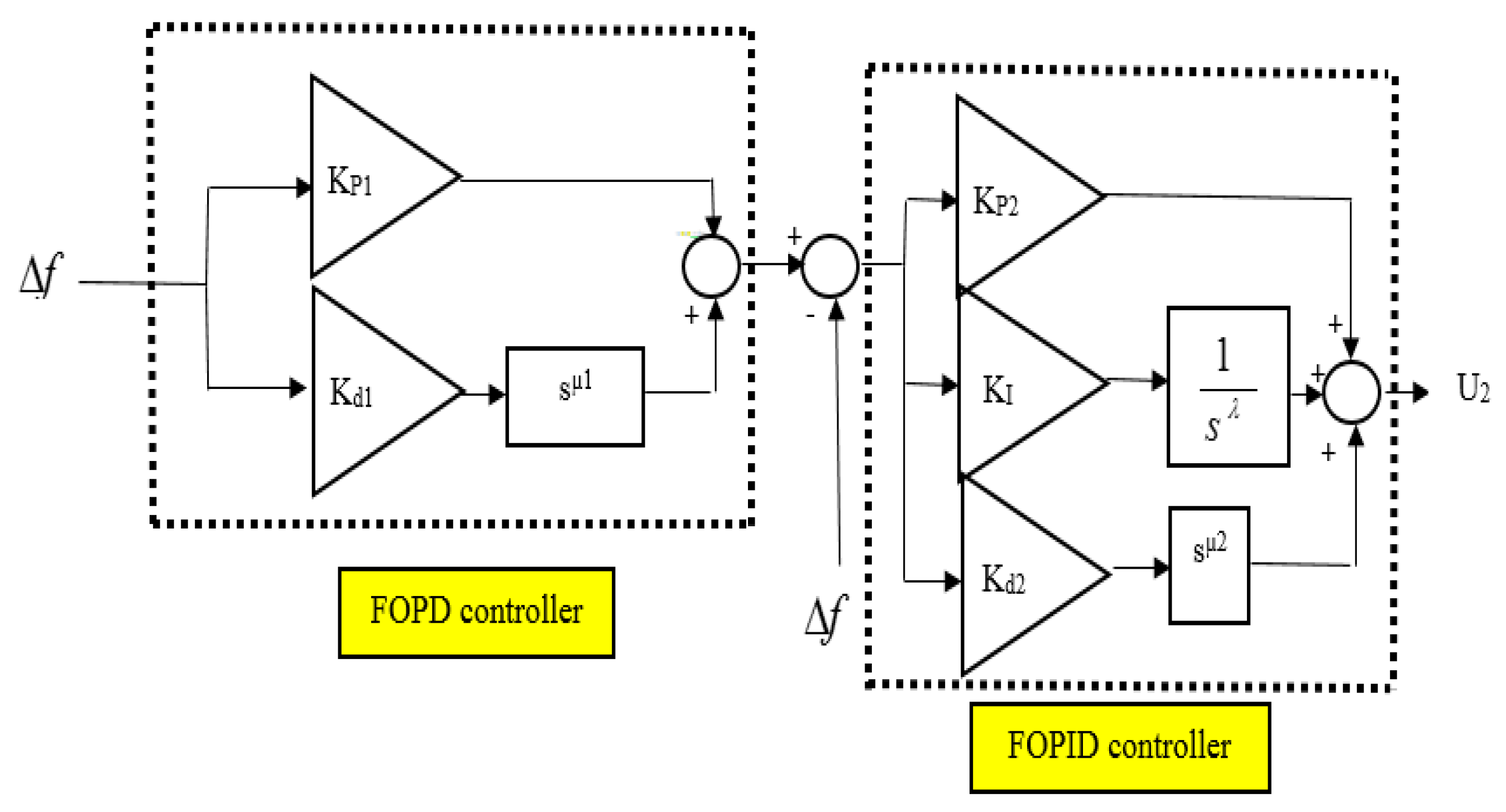
3.1. Structure of the Proposed Controller

The FOPD–FOPID cascaded controller has been intricately designed to enhance the stability of frequency within power systems that incorporate wind turbines. Its primary objective is to minimize deviations in frequency caused by load disturbances, disruptions from wind turbines, and uncertainties in power system parameters. This elaborate controller consists of two components: the FOPD controller and the FOPID controller. The FOPD controller primarily determines the outcome, while the FOPID controller shapes and guides it by adjusting the reference signal. In this proposed control framework, the FOPD controller is referred to as the main, primary, or external controller, and the FOPID controller is referred to as the internal, secondary, or sub-controller. These components work synergistically, as depicted in Figure 3, to establish cohesive coordination between the LFC system and the SMES. Figure 3 illustrates the suggested setup of the cascaded controller, which facilitates the orchestration of the inner loop dynamics through Equation (3). Equation (3) succinctly represents the transfer function that exclusively encapsulates the inner loop dynamics, as demonstrated in Figure 3:

$$Y_2(s)=M_2(s)U_2(s)$$

(3)

In Equation (3), M₂(s) embodies the transfer function of the internal process, whereas U₂(s) signifies the input signal directed towards said process. The principal controller (FOPD), situated in the outer layer, adeptly curtails any oscillations pertaining to frequency and mitigates external interferences. Equation (4) reveals the transfer function characterizing the outer loop’s operation:

$$Y(s)=M_1(s)U_1(s)$$

(4)

where M₁(s) symbolizes the transfer function of the external process, while U₁(s) stands for the input signal directed towards said process. As Figure 3 illustrates, N₂(s) denotes the FOPID controller found in the inner layer, whereas N₁(s) represents the FOPD controller situated in the outer layer. The transfer functions of both FOPD and FOPID controllers are demonstrated through Equations (5) and (6):

$$N_1(s)=K_{P1}+K_{d1}{s}^{{\mu }_1}$$

(5)

$$N_2(s)=K_{P2}+K_I{s}^{-\lambda }+K_{d2}{s}^{{\mu }_2}$$

(6)

Figure 4 shows the inside structure of the FOPD-FOPID controller.

The settings of the suggested controller are found by making the ISE objective function as small as possible by using the DOSA method. Equation (7) shows the main goal of ISE. The limits or boundaries of the objective functions are represented by Equation (8):

$$ISE={\displaystyle \underset{0}{\overset{t_s}{\int }}{(\Delta f)}^{2}dt}$$

(7)

$$\begin{array}{l}{K}_{P1,\min }\le K_{P1}\le K_{P1,\max }\\ K_{d1,\min }\le K_{d1}\le K_{d1,\max }\\ {\mu }_{1,\min }\le {\mu }_1\le {\mu }_{1,\max }\\ K_{P2,\min }\le K_{P2}\le K_{P2,\max }\\ K_{I,\min }\le K_I\le K_{I,\max }\\ K_{d2,\min }\le K_{d2}\le K_{d2,\max }\\ {\lambda }_{\min }\le \lambda \le {\lambda }_{\max }\\ {\mu }_{2,\min }\le {\mu }_2\le {\mu }_{2,\max }\end{array}$$

(8)

3.2. FOPID Controller

Based on the generalized non-integer order fundamental operator, Fractional-order Systems are established (Equation (9)) [27]:

$$a{D}_t^{\psi }=\left\{\begin{array}{ll}\frac{d^{\psi }}{d{t}^{\psi }}& \psi >0\\ 1& \psi =0\\ {\displaystyle \underset{a}{\overset{t}{\int }}{(dt)}^{-\psi }}& \psi <0\end{array}\right.$$

(9)

The limits of the operation, denoted by a and t, are considered in fractional-order systems. It is typically assumed that $\psi \in R$, although it can also be a complex number. Various definitions of the integral-differential operator have been formulated. The Grünwald–Letnikov definition is commonly employed in the application of FOPID due to its suitability for numerically evaluating fractional order derivatives (Equation (10)) [27]:

$$a{D}_t^{\psi }f(t)=\underset{h\to 0}{{\displaystyle \lim }}\frac{1}{h^{\psi }}{\displaystyle \sum _{j=0}^k{(-1)}^j}\left(\begin{array}{l}\psi \\ j\end{array}\right)f(t-jh)$$

(10)

In Equation (10), a is set to 0, t is equal to kh, where k represents the number of computation steps, and h denotes the step size. Considering zero initial conditions, the Laplace transform of the $\psi$-order derivative is given by Equation (11) [27]:

$${\displaystyle \underset{0}{\overset{\infty }{\int }}{e}^{-st}{}_0{D}_t^{\psi }f(t)dt}=s^{\psi }F(s)$$

(11)

In Equation (11), $\psi \in R^{+}$, and s is the usual Laplace variable. The PI ^λD^µ controller, also known as the generalized FOPID controller [27,28,29], incorporates an integrator of order λ and a differentiator of order µ. The time domain equation for the FOPID controller can be expressed as Equation (12). In Equation (12), the terms D^−λ e(t) and D^µ e(t) denote the fractional-order integral and fractional-order derivative, respectively:

$$u_x(t)=K_{P}e(t)+K_i{D}^{-\lambda }e(t)+K_d{D}^{\mu }e(t)$$

(12)

3.3. Developed Owl Search Algorithm (DOSA)

The DOSA is a state-of-the-art meta-heuristic algorithm that offers several advantages over other algorithms such as GTO, MSA, PSO, and ABC. These advantages include: (1) Efficient Search: The DOSA utilizes the owl search behavior, enabling efficient exploration of the search space. The algorithm is designed to strike a balance between exploration and exploitation, facilitating fast convergence towards optimal solutions. (2) Global Optimization: The DOSA is a global optimization algorithm, capable of seeking the global optimum without getting trapped in local optima. This characteristic makes it well-suited for tackling complex optimization problems with multiple solution vertices. (3) Robustness: The DOSA exhibits robustness against noise and uncertainty in the objective function. It adapts effectively to noisy and dynamic environments, making it suitable for real-world applications where the objective function may change over time. (4) Minimal Control Parameters: Compared to other optimization algorithms, the DOSA requires a reduced number of control parameters. This simplifies the tuning process, reduces computational load, and facilitates implementation across various domains. (5) Fast Convergence Speed: The DOSA demonstrates fast convergence in a wide range of optimization problems. It efficiently converges towards near-optimal solutions, significantly reducing the computational time required for finding high-quality solutions. These advantages have been documented in various studies [47,48,49], highlighting the effectiveness and versatility of the DOSA algorithm.

Similar to the application of other meta-heuristic algorithms in electrical engineering [50,51,52], its execution is initiated by fortuitously selecting a population. Within this algorithm, said population symbolizes the owls’ positioning amidst the forest trees exemplifying the search space. Given that the number of random populations is represented as “n” and the forest is considered as a d-dimensional search space in this algorithm, visually expressing the chance placements of these nocturnal creatures within an n × d matrix can be encapsulated with Equation (13) [47]:

$$x={\left[\begin{array}{ccc}{x}_{1,1}& \dots & x_{1,d}\\ .& & .\\ .& & .\\ x_{n,1}& \dots & x_{n,d}\end{array}\right]}_{n\times d}$$

(13)

where the component x_i,j in the matrix defines the jth variable (dimension) of ith owl. In the owl search algorithm, the term “ith owl” refers to the owl that is being considered or processed in the ith iteration or step of the algorithm. The owl search algorithm is a heuristic search algorithm inspired by the behavior of owls when hunting prey. It uses a combination of local search and global exploration to find an optimal solution. In each iteration, the algorithm evaluates the current owl (ith owl) and updates its position based on certain rules and heuristics. The process continues until a satisfactory solution is found or the search space has been fully explored. To make an introductory state of uniform dissemination, Equation (14) is utilized [47,48,49]:

$$x_i=x_l+(x_l+x_u)Z(0,1)$$

(14)

In Equation (14), X_i could be irregular and uniform numbers between [0, 1], and x_u and x_l are the upper and lower bounds of the ith owl within the jth measurement.

In the realm of mathematical equations, specifically Equation (14), Z(0,1) stands as an intriguing integer that embraces both randomness and uniformity within its numerical essence, constrained between the ethereal boundaries [0,1]. Furthermore, the mysterious confines of x_u and x_l possess a duality and significance in defining not just any owl’s position within this enigmatic forest, but rather the profound location it assumes in the jth dimension. As we venture further into comprehending this intricate web of numerics and spatial relations, one is compelled to ponder the cost associated with these owls’ chosen abodes in the forest. Illuminatingly explained through Equation (15) [47,48,49,50], this particular measure serves as a window into understanding how nature has woven together factors such as distance or resources so crucial to determine what truly befits an owl’s dwelling and how they impact its existence:

$$f=\left[\begin{array}{l}{f}_1(\left[x_{1,1},x_{1,2},\dots ,x_{1,d}\right])\\ .\\ .\\ .\\ f_n(\left[x_{n,1},x_{n,2},\dots ,x_{n,d}\right])\end{array}\right]$$

(15)

The owl’s position is contingent upon the magnitude of the sounds it detects through its delicate ears. In this instance, the owl that receives the most intense sound is considered superior because it signifies proximity to the desired goal. The normalized intensity value for each respective owl, denoted by i, will be utilized to revise its position, as derived from Equation (16) [46]:

$$\left\{\begin{array}{l}{I}_i=\frac{f_i-w}{b-w}\\ b=\max \hspace{0.17em}\hspace{0.17em}{f}_m\\ {}^{m\in 1,\dots ,n}\\ w=\min \hspace{0.17em}\hspace{0.17em}{f}_m\\ {}^{m\in 1,\dots ,n}\end{array}\right.$$

(16)

The measurement of prey distance for each individual owl can be acquired by applying Equation (17) [46,47,48]:

$$D_i=\sqrt{{\displaystyle \sum _i{(x_i-L)}^2}}$$

(17)

Equation (17) encompasses the representation of prey positions (L), retrieved through the utilization of the most adept owl. The owl search algorithm postulates the existence of prey amidst the forest as a premise for global optimization. During their pursuit, owls advance meticulously towards their target with gradual aerial movement. The extent to which each ith owl undergoes transformation is delineated in Equation (18) [47,48,49,50]:

$$C_i=\frac{I_i}{D_i^2}+R_n$$

(18)

In the Equation (18), the variable $4\pi D_i^2$ has been substituted with $D_i^2$, while $R_n$ represents a stochastic element introduced in order to enhance the model’s practicality. As the prey transitions from one location to another, it becomes imperative for the owls to cautiously shift closer towards their target. This algorithm encompasses a mechanism by which the alteration in prey position is determined through probability. Consequently, Equation (19) serves as an update mechanism demonstrating how the new positions of the owls relative to those of their intended prey are depicted:

$$x_i^{t+1}=\left\{\begin{array}{l}{x}_i^t+\beta C_i\left|\alpha L-x_i^t\right|,\hspace{0.17em}\hspace{0.17em}{p}_{pm}<0.5\\ x_i^t-\beta C_i\left|\alpha L-x_i^t\right|,\hspace{0.17em}\hspace{0.17em}\hspace{0.17em}{p}_{pm}>0.5\end{array}\right.$$

(19)

Equation (19) introduces the concept of $p_{pm}$ as a representation of prey position change probability, while $\alpha$ and $\beta$ are uniformly distributed random numbers that range from 0 to 0.5 and 0 to 1.9, respectively. This unique characteristic of the owl search algorithm sets it apart from other algorithms, providing superior reliability. While the owl search algorithm is relatively new among optimization algorithms, it occasionally encounters a drawback in becoming trapped within the confines of local optima. Nonetheless, this flaw presents an opportunity for early convergence-inspired solutions. Aware of these limitations, modifications have been implemented to enhance both the performance and effectiveness of the owl search algorithm when confronted with local optima traps. The incorporation of chaos theory has gained traction recently due to its profound influence on modeling effects of nonlinear dynamics; optimization falls within this sphere, susceptible to such influences. By default, in the conventional implementation of the owl search algorithm, only variable $\beta$ serves as a source for randomness within each iteration. However, including variable $\beta$ introduces an alternative pathway towards early convergence by expanding its role throughout iterations. In order to avert premature convergence within the system, the implementation of a tumultuous technique known as Singer mapping is employed [53]. This strategy involves treating the obscure variable as a customary equation in conformity with Equation (20):

$${\beta }_{i+1}=1.07(7.9{\beta }_i-23.3{\beta }_i^2+28.7{\beta }_i^3-13.3{\beta }_i^4)$$

(20)

Furthermore, an alternative approach to enhance initial convergence in the owl search algorithm entails incorporating Lévy flight. The inclusion of random navigation constitutes an integral facet of this methodology for effectively regulating local search. The mathematical representation of this technique can be found in Equations (21) through (23) [53]:

$$Le(w)\approx w^{-1-\tau }$$

(21)

$$w=\frac{A}{{\left|B\right|}^{\frac{1}{\tau }}}$$

(22)

$${\sigma }^2={\left\{\frac{\Gamma (1+\tau )}{\tau \Gamma ((1+\tau )/2)}\frac{\sin (\pi \tau /2)}{2^{(1+\tau )/2}}\right\}}^{\frac{2}{\tau }}$$

(23)

In Equations (21)–(23), $\tau$ represents a number that can be between 0 and 2. The letter w stands for a small measurement size. The letter $\Gamma (0)$ represents a mathematical operation called the gamma function. The letters $A/B\approx N(0,{\sigma }^2)$ indicate that the values are taken from a group where each value is chosen randomly from a bell-shaped curve, with the middle value being zero. The range of values for this group is ${\sigma }^2$. Using Equation (24), we can find the new location of the owls based on the given connections.

$$x_i^{t+1}=\left\{\begin{array}{l}{x}_i^t+\beta C_i\left|\alpha L-x_i^t\right|Le(\delta ),\hspace{0.17em}\hspace{0.17em}{p}_{pm}<0.5\\ x_i^t-\beta C_i\left|\alpha L-x_i^t\right|Le(\delta ),\hspace{0.17em}\hspace{0.17em}\hspace{0.17em}{p}_{pm}>0.5\end{array}\right.$$

(24)

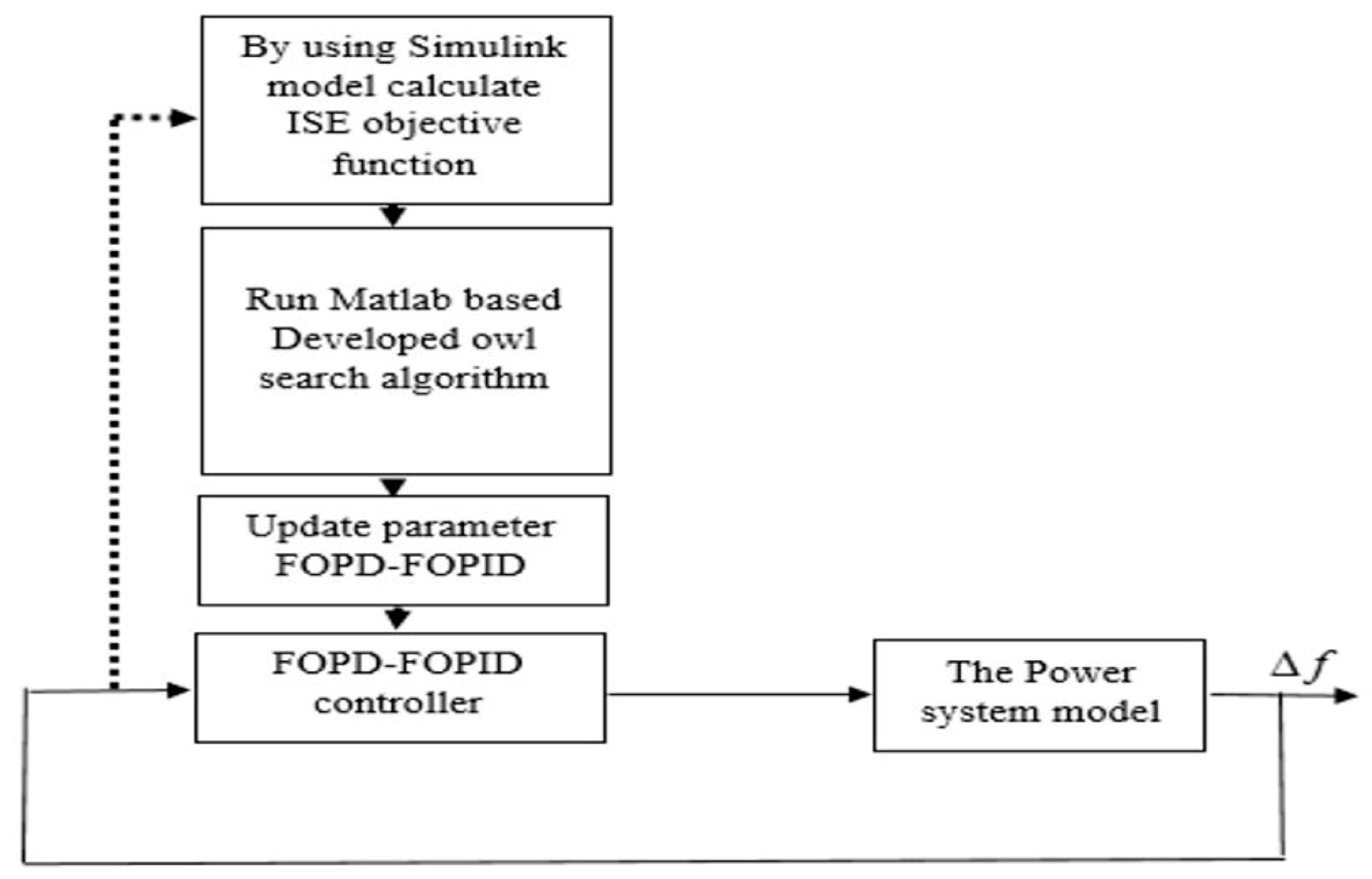
3.4. Design Process of the Proposed Controller Utilizing the DOSA

To improve the performance of the FOPD–FOPID controller for the coordinated control of the LFC system and SMES, we need to follow these steps:

(1)

Definition of the objective function: The objective function is a mathematical representation of the goal we want to achieve in this problem. It is determined using Equation (7).

(2)

Constraints are rules that help us find the best values for the FOPD–FOPID controller. We define these rules using Equation (8).

(3)

Creating the first group of owls: In this step, we create a starting population of owls. Each owl in this group has a different number for each FOPD–FOPID controller setting.

(4)

Analyzing the population: The first group of individuals is assessed using a specific measurement called the objective function. We calculate the value of the objective function for every owl.

(5)

Choosing the best owls: We select the owls with the highest scores to be part of the next generation.

(6)

During this stage, new owls are made for the future generation. This work can be completed by adding or subtracting big owls, or by using random actions.

(7)

Assessment of the new group of owls: The new group of owls is judged based on the objective function.

(8)

Doing steps 5 to 7 again and again until certain stopping conditions are satisfied, like reaching the desired value of the goal function or finishing a certain number of repetitions.

(9)

Choosing the top owl: Once all the rounds are done, the owl with the highest value of the main goal is picked as the best answer. This owl gives the best values for the settings of the FOPD–FOPID controller.

The image depicted in Figure 5 illustrates the utilization of the DOSA to optimize the parameters of the FOPD–FOPID controller. This optimization process is specifically aimed at achieving coordinated control of the LFC system and SMES.

4. Simulation Results and Discussion

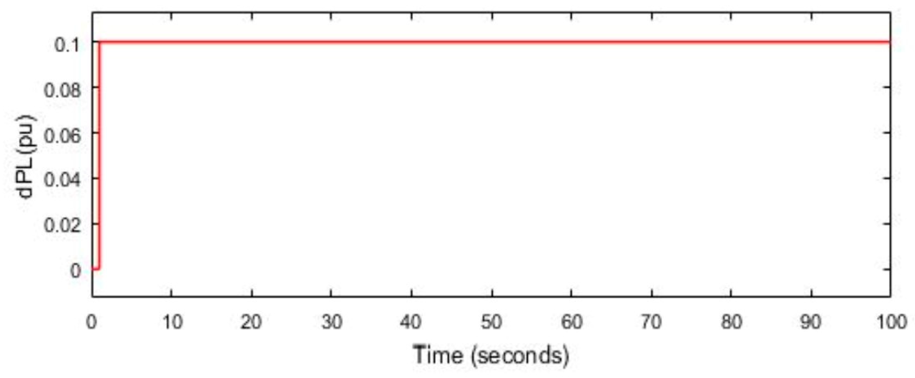
In this particular section, the system under study has undergone testing in the presence of a wind turbine across four distinct scenarios. The first scenario (1) is divided into two parts: firstly, an evaluation of the efficiency and adaptability of the DOSA for optimizing the FOPD–FOPID controller parameters takes place alongside a comparison with other algorithms such as MSA, PSO, ABC, and GTO. Secondly, various methods incorporating the proposed DOSA–FOPD–FOPID controller are utilized to compare performance including LFC and SMES based on a robust controller (Controller 1); LFC and SMES based on the MSA–PID controller (Controller 2); LFC based solely on the MSA–PID controller with SMES (Controller 3); and finally, LFC based on the MSA–PID controller without SMES (Controller 4). These comparisons are made while accounting for both load disruptions and wind turbine disruptions. In scenario (2), the proposed method is being compared to several other methods, namely Controller 1, Controller 2, Controller 3, and Controller 4. The aim is to evaluate its performance in handling load disruptions and wind turbine disruptions. Moving on to scenarios (3) and (4), the performance of the proposed method is assessed alongside the mentioned methods. In addition to load disruptions and wind turbine disruptions, these scenarios also consider uncertainties related to power system parameters and disruptions caused by renewable energy sources such as wind turbines.

4.1. Scenario (1)

In this scenario, the power system being analyzed (Figure 2) experiences a disruption in its load with an amplitude of ΔP_L = 0.1 pu at t = 1 s, as depicted in Figure 6. The fundamental parameters pertaining to the DOSA and FOPD–FOPID cascaded controller are presented in

Table 2. Fundamental parameters pertaining to the DOSA and FOPD–FOPID cascaded controller.

Parameter	Value	Parameter	Value
Population of owls	100	$K_{P1,\min },K_{d1,\min },K_{P2,\min },K_{I,\min },K_{d2,\min }$	0
Forest range for capacity	[0,1000]	$K_{P1,\max },K_{d1,\max },K_{P2,\max },K_{I,\max },K_{d2,\max }$	100
$\alpha$	1	${\lambda }_{\min },{\mu }_{1,2,\min }$	0
Iterations (stop criteria)	100	${\lambda }_{\max },{\mu }_{1,2,\max }$	1

. Figure 7 illustrates the optimization process of FOPD–FOPID controller parameters using different algorithms, namely DOSA, MSA, PSO, ABC, and GTO. The objective function utilized is ISE. As demonstrated by Figure 7, it can be observed that the DOSA algorithm yields a swifter convergence rate than the others mentioned. In terms of ISE values obtained from the respective algorithms (DOSA: 6.8 × 10⁻⁶; GTO: 9 × 10⁻⁶; MSA: 9.1 × 10⁻⁶; ABC: 9.9 × 10⁻⁶; and PSO: 10 × 10⁻⁶), they are displayed in numeric format for easier comprehension. In

Table 3. Values of parameters of the FOPD–FOPID controller using different algorithms.

Controller	KP1	µ1	Kd1	KP2	KI	Kd2	λ	µ2	ISE
DOSA–FOPD–FOPID	91.55	0.65	88.91	98.22	91.44	86.35	0.56	0.74	6.8 × 10−6
GTO–FOPD–FOPID	89.13	0.58	83.66	89.55	83.87	84.18	0.40	0.42	9 × 10−6
MSA–FOPD–FOPID	85.82	0.62	87.44	92.34	90.56	75.79	0.46	0.40	9.1 × 10−6
ABC–FOPD–FOPID	68.23	0.49	91.23	86.25	78.45	76.39	0.43	0.38	9.9 × 10−6
PSO–FOPD–FOPID	70.65	0.47	81.77	75.21	79.92	71.36	0.39	0.48	10 × 10−6

, the values of optimized parameters of the FOPD–FOPID controller considering the ISE objective function for DOSA, GTO, MSA, ABC, and PSO algorithms are shown. According to Figure 7 and Table 3, the DOSA can be used to optimize the FOPD–FOPID controller parameters. In this scenario, load disruptions and wind turbine disruptions have been applied to the power system according to Figure 8. In Figure 9a–e, the FR of the power system using different control methods to load and wind turbine disruptions is shown. According to Figure 9a, the MFD and ST based on LFC and SMES based on the proposed controller (optimized FOPD–FOPID controller using the DOSA) is equal to 0.0009 Hz and 4.2 s, respectively. The MFD and ST based on controller 1 are equal to 0.0018 Hz and 5 s, respectively; the MFD and ST based on controller 2 are equal to 0.0173 Hz and 19 s, respectively; the MFD and ST based on controller 3 are equal to 0.021 Hz and 38 s, respectively; and the MFD and ST based on controller 4 are equal to 0.0476 Hz and 90 s, respectively (Figure 9b–e). Based on the outcomes of this particular scenario, it is evident that the proposed controller surpasses its counterparts in effectively mitigating power system deviations, and it has also reduced the ST of frequency deviations caused by disruptions on the power system.

4.2. Scenario (2)

In this scenario, load disruptions and wind turbine disruptions have been applied to the power system according to Figure 10. In Figure 11a–e, the FR of the power system using different control methods to load disruptions and wind turbine disruptions is shown. According to Figure 11a, the MFD and ST based on the proposed controller (optimized FOPD–FOPID controller using the DOSA) are equal to 0.0007 Hz and 3.55 s, respectively. The MFD and ST based on controller 1 are equal to 0.0015 Hz and 4.46 s, respectively; the MFD and ST based on controller 2 are equal to 0.0081 Hz and 21 s, respectively; the MFD and ST based on controller 3 are equal to 0.0129 Hz and 37 s, respectively; and the MFD and ST based on controller 4 are equal to 0.0256 Hz and 45 s, respectively (Figure 11b–e). Based on these results, the proposed controller performs better in reducing the deviations of the power system than the other mentioned controllers, and it also reduces the settling time of the frequency deviations caused by disruptions in the power system.

4.3. Scenario (3)

In this scenario, load disruptions and wind turbine disruptions have been applied to the power system according to Figure 10. In this scenario, slight uncertainty related to the power system parameters is considered in the system inertia (H = −25%). In Figure 12a–e, the frequency response of the power system to load disruptions, wind turbine disruptions and mild uncertainty related to the system parameters are shown. According to Figure 12a, the MFD and ST based on the proposed controller (optimized FOPD–FOPID controller using the DOSA) are equal to 0.00075 Hz and 3.76 s, respectively. The MFD and ST based on controller 1 are equal to 0.00163 Hz and 4.49 s, respectively; the MFD and ST based on controller 2 are equal to 0.0106 Hz and 24 s, respectively; the MFD and ST based on controller 3 are equal to 0.017 Hz and 42 s, respectively; and the MFD and ST based on controller 4 are equal to 0.0336 Hz and 48 s, respectively (Figure 12b–e). Based on the results obtained in this section, the proposed controller performs better in reducing the deviations of the power system compared to the other mentioned controllers and reduces the ST of the frequency deviations caused by the disruptions in the power system and is resistant to the mild uncertainty related to the system parameters.

4.4. Scenario (4)

In this scenario, load disruptions and wind turbine disruptions have been applied to the power system according to Figure 10. In this scenario, severe uncertainty related to the power system parameters is considered in the system inertia (H = −50%). In Figure 13a–e, the FR of the power system to load disruptions, wind turbine disruptions, and severe uncertainty related to the system parameters are shown. According to Figure 13a, the MFD and ST based on the proposed controller (optimized FOPD–FOPID controller using the DOSA) are equal to 0.00079 Hz and 3.93 s, respectively. The MFD and ST based on controller 1 are equal to 0.00172 Hz and 4.58 s, respectively; the MFD and ST based on controller 2 are equal to 0.0157 Hz and 25 s, respectively; and the MFD and ST based on controller 3 with SMES are equal to 0.0197 Hz and 46 s, respectively (Figure 13b–d). According to Figure 13e, the FR of the power system is unstable against severe disruptions using LFC based on controller 4, and this control method does not have the ability to maintain frequency stability against severe disruptions related to the parameters of the power system. According to the results of scenario (4), the proposed controller performs better in reducing the deviations of the power system than the other mentioned controllers; it reduces the ST of the frequency deviations caused by disruptions in the power system and is resistant to the severe uncertainty related to the system parameters. In

Table 4. Performance results of different control methods for four scenarios.

Controller		Scenario (1)	Scenario (2)	Scenario (3)	Scenario (4)
Proposed controller	MO (Hz)	0.0001	0.00035	0.00037	0.00038
	MU (Hz)	0.0009	0.0007	0.00075	0.00079
	ST (s)	4.2	3.55	3.76	3.93
Controller 1	MO (Hz)	0.0004	0.0008	0.0009	0.0010
	MU (Hz)	0.00184	0.00152	0.001631	0.001724
	ST (s)	5.05	4.461	4.492	4.492
Controller 2	MO (Hz)	0.00421	0.00341	0.0053	0.0092
	MU (Hz)	0.01734	0.00816	0.01066	0.01578
	ST (s)	19.03	21.24	24.53	25.22
Controller 3	MO (Hz)	0.00643	0.00582	0.0127	0.0146
	MU (Hz)	0.0214	0.01291	0.01708	0.01975
	ST (s)	38.12	37.39	42.11	46.25
Controller 4	MO (Hz)	0.0476	0.023	0.0367	---
	MU (Hz)	0.04667	0.02565	0.03363	---
	ST (s)	90.1	45.03	48.21	---

, performance results of different control methods for 4 scenarios are shown.

5. Conclusions

In this paper, a robust control method has been designed for the coordinated control of LFC and SMES using the FOPD–FOPID controller. The DOSA algorithm, which has many advantages over other optimization algorithms, was used to adjust the parameters of the proposed controller. The proposed method in this paper is compared with other methods presented in the field of power system frequency control in the presence of wind turbines. The proposed method was able to improve the MFD and ST related to frequency deviations in the power system caused by load disturbances and wind turbine disturbances by 50% and 17%, respectively, compared to other methods presented in this field (frequency control). The proposed method has been able to improve the MFD and ST related to frequency deviations in the power system caused by load disturbances, wind turbine disturbances, and slight uncertainty of parameters (H = −%25) by 45% and 18%, respectively (compared to other methods presented in the field of frequency control). The proposed method improved the MFD and ST related to frequency deviations in the power system caused by load disturbances, wind turbine disturbances, and extreme uncertainty of parameters (H = −%50) by 45% and 18%, respectively (compared to other methods presented in the field of frequency control). To continue the work of this paper in the future, several suggestions can be made, including: (1) Combining the FOPD–FOPID controller with a neural network and using it in different parts of the power system, (2) Investigating the possibility of using the FOPD–FOPID controller in power systems Smart, (3) checking the performance of the FOPD–FOPID controller in case of faults in the power system and defects in other system components.

References

1. Ukaegbu, U.; Tartibu, L.; Lim, C.W. Multi-Objective Optimization of a Solar-Assisted Combined Cooling, Heating and Power Generation System Using the Greywolf Optimizer. Algorithms 2023, 16, 463. [Google Scholar] [CrossRef]
2. Yang, G.; Yi, H.; Chai, C.; Huang, B.; Zhang, Y.; Chen, Z. Predictive current control of boost three-level and T-type inverters cascaded in wind power generation systems. Algorithms 2018, 11, 92. [Google Scholar] [CrossRef]
3. Zheng, C.; Eskandari, M.; Li, M.; Sun, Z. GA−Reinforced Deep Neural Network for Net Electric Load Forecasting in Microgrids with Renewable Energy Resources for Scheduling Battery Energy Storage Systems. Algorithms 2022, 15, 338. [Google Scholar] [CrossRef]
4. Eskandari, M.; Rajabi, A.; Savkin, A.V.; Moradi, M.H.; Dong, Z.Y. Battery energy storage systems (BESSs) and the economy-dynamics of microgrids: Review, analysis, and classification for standardization of BESSs applications. J. Energy Storage 2022, 55, 105627. [Google Scholar] [CrossRef]
5. Amiri, F.; Eskandari, M.; Moradi, M.H. Virtual Inertia Control in Autonomous Microgrids via a Cascaded Controller for Battery Energy Storage Optimized by Firefly Algorithm and a Comparison Study with GA, PSO, ABC, and GWO. Energies 2023, 16, 6611. [Google Scholar] [CrossRef]
6. Amiri, F.; Hatami, A. Load frequency control for two-area hybrid microgrids using model predictive control optimized by grey wolf-pattern search algorithm. Soft Computing 2023, 27, 18227–18243. [Google Scholar] [CrossRef]
7. Paducel, I.; Safirescu, C.O.; Dulf, E.-H. Fractional Order Controller Design for Wind Turbines. Appl. Sci. 2022, 12, 8400. [Google Scholar] [CrossRef]
8. Lu, L.; Saborío-Romano, O.; Cutululis, N.A. Reduced-Order-VSM-Based Frequency Controller for Wind Turbines. Energies 2021, 14, 528. [Google Scholar] [CrossRef]
9. Abumeteir, H.A.; Vural, A.M. Design and Optimization of Fractional Order PID Controller to Enhance Energy Storage System Contribution for Damping Low-Frequency Oscillation in Power Systems Integrated with High Penetration of Renewable Sources. Sustainability 2022, 14, 5095. [Google Scholar] [CrossRef]
10. Idir, A.; Canale, L.; Bensafia, Y.; Khettab, K. Design and Robust Performance Analysis of Low-Order Approximation of Fractional PID Controller Based on an IABC Algorithm for an Automatic Voltage Regulator System. Energies 2022, 15, 8973. [Google Scholar] [CrossRef]
11. Tan, W. Tuning of PID load frequency controller for power systems. Energy Convers. Manag. 2009, 50, 1465–1472. [Google Scholar] [CrossRef]
12. Hussain, I.; Das, D.C.; Latif, A.; Sinha, N.; Hussain, S.S.; Ustun, T.S. Active power control of autonomous hybrid power system using two degree of freedom PID controller. Energy Rep. 2022, 8, 973–981. [Google Scholar] [CrossRef]
13. Shabani, H.; Vahidi, B.; Ebrahimpour, M. A robust PID controller based on imperialist competitive algorithm for load-frequency control of power systems. ISA Trans. 2013, 52, 88–95. [Google Scholar] [CrossRef] [PubMed]
14. Bahgaat, N.K.; El-Sayed, M.I.; Hassan, M.M.; Bendary, F.A. Load frequency control in power system via improving PID controller based on particle swarm optimization and ANFIS techniques. In Research Methods: Concepts, Methodologies, Tools, and Applications; IGI Global: Hershey, PA, USA, 2015; pp. 462–481. [Google Scholar]
15. Sambariya, D.K.; Fagna, R. A novel Elephant Herding Optimization based PID controller design for Load frequency control in power system. In Proceedings of the 2017 International Conference on Computer, Communications and Electronics (Comptelix), Jaipur, India, 1–2 July 2017; pp. 595–600. [Google Scholar]
16. Bernard, M.; Musilek, P. Ant-based optimal tuning of PID controllers for load frequency control in power systems. In Proceedings of the 2017 IEEE Electrical Power and Energy Conference (EPEC), Saskatoon, SK, Canada, 22–25 October 2017; pp. 1–6. [Google Scholar]
17. Osinski, C.; Leandro, G.V.; da Costa Oliveira, G.H. Fuzzy PID controller design for LFC in electric power systems. IEEE Lat. Am. Trans. 2019, 17, 147–154. [Google Scholar] [CrossRef]
18. Sahu, B.K.; Pati, T.K.; Nayak, J.R.; Panda, S.; Kar, S.K. A novel hybrid LUS-TLBO optimized fuzzy-PID controller for load frequency control of multi-source power system. Int. J. Electr. Power Energy Syst. 2016, 74, 58–69. [Google Scholar] [CrossRef]
19. Sahu, R.K.; Sekhar, G.C.; Panda, S. DE optimized fuzzy PID controller with derivative filter for LFC of multi source power system in deregulated environment. Ain Shams Eng. J. 2015, 6, 511–530. [Google Scholar] [CrossRef]
20. Sahu, R.K.; Panda, S.; Yegireddy, N.K. A novel hybrid DEPS optimized fuzzy PI/PID controller for load frequency control of multi-area interconnected power systems. J. Process Control 2014, 24, 1596–1608. [Google Scholar] [CrossRef]
21. Joshi, M.; Sharma, G.; Bokoro, P.N.; Krishnan, N. A fuzzy-PSO-PID with UPFC-RFB solution for an LFC of an interlinked hydro power system. Energies 2022, 15, 4847. [Google Scholar] [CrossRef]
22. Chen, G.; Li, Z.; Zhang, Z.; Li, S. An improved ACO algorithm optimized fuzzy PID controller for load frequency control in multi area interconnected power systems. IEEE Access 2019, 8, 6429–6447. [Google Scholar] [CrossRef]
23. Sahu, R.K.; Panda, S.; Pradhan, P.C. Design and analysis of hybrid firefly algorithm-pattern search based fuzzy PID controller for LFC of multi area power systems. Int. J. Electr. Power Energy Syst. 2015, 69, 200–212. [Google Scholar] [CrossRef]
24. Fathy, A.; Kassem, A.M.; Abdelaziz, A.Y. Optimal design of fuzzy PID controller for deregulated LFC of multi-area power system via mine blast algorithm. Neural Comput. Appl. 2020, 32, 4531–4551. [Google Scholar] [CrossRef]
25. Sekhar, G.C.; Sahu, R.K.; Baliarsingh, A.K.; Panda, S. Load frequency control of power system under deregulated environment using optimal firefly algorithm. Int. J. Electr. Power Energy Syst. 2016, 74, 195–211. [Google Scholar] [CrossRef]
26. Tammam, M.A.; Aboelela, M.A.S.; Moustafa, M.A.; Seif, A.E.A. Fuzzy like PID controller tuning by multiobjective genetic algorithm for load frequency control in nonlinear electric power systems. Int. J. Adv. Eng. Technol. 2012, 5, 572. [Google Scholar]
27. Sorcia-Vázquez, F.D.J.; Rumbo-Morales, J.Y.; Brizuela-Mendoza, J.A.; Ortiz-Torres, G.; Sarmiento-Bustos, E.; Pérez-Vidal, A.F.; Osorio-Sánchez, R. Experimental Validation of Fractional PID Controllers Applied to a Two-Tank System. Mathematics 2023, 11, 2651. [Google Scholar] [CrossRef]
28. Sondhi, S.; Hote, Y.V. Fractional order PID controller for load frequency control. Energy Convers. Manag. 2014, 85, 343–353. [Google Scholar] [CrossRef]
29. Kumar, A.; Pan, S. Design of fractional order PID controller for load frequency control system with communication delay. ISA Trans. 2022, 129, 138–149. [Google Scholar] [CrossRef]
30. Taher, S.A.; Fini, M.H.; Aliabadi, S.F. Fractional order PID controller design for LFC in electric power systems using imperialist competitive algorithm. Ain Shams Eng. J. 2014, 5, 121–135. [Google Scholar] [CrossRef]
31. Zamani, A.; Barakati, S.M.; Yousofi-Darmian, S. Design of a fractional order PID controller using GBMO algorithm for load-frequency control with governor saturation consideration. ISA Trans. 2016, 64, 56–66. [Google Scholar] [CrossRef]
32. Babaei, F.; Safari, A. SCA based fractional-order PID controller considering delayed EV aggregators. J. Oper. Autom. Power Eng. 2020, 8, 75–85. [Google Scholar]
33. Ahuja, A.; Narayan, S.; Kumar, J. Robust FOPID controller for load frequency control using Particle Swarm Optimization. In Proceedings of the 2014 6th IEEE Power India International Conference (PIICON), Delhi, India, 5–7 December 2014; pp. 1–6. [Google Scholar]
34. Daraz, A.; Malik, S.A.; Basit, A.; Aslam, S.; Zhang, G. Modified FOPID controller for frequency regulation of a hybrid interconnected system of conventional and renewable energy sources. Fractal Fract. 2023, 7, 89. [Google Scholar] [CrossRef]
35. Zaid, S.A.; Kassem, A.M.; Alatwi, A.M.; Albalawi, H.; AbdelMeguid, H.; Elemary, A. Optimal Control of an Autonomous Microgrid Integrated with Super Magnetic Energy Storage Using an Artificial Bee Colony Algorithm. Sustainability 2023, 15, 8827. [Google Scholar] [CrossRef]
36. Shayeghi, H.; Jalili, A.; Shayanfar, H.A. A robust mixed H2/H∞ based LFC of a deregulated power system including SMES. Energy Convers. Manag. 2008, 49, 2656–2668. [Google Scholar] [CrossRef]
37. Pappachen, A.; Fathima, A.P. Load frequency control in deregulated power system integrated with SMES-TCPS combination using ANFIS controller. Int. J. Electr. Power Energy Syst. 2016, 82, 519–534. [Google Scholar] [CrossRef]
38. Sudha, K.R.; Santhi, R.V. Load frequency control of an interconnected reheat thermal system using type-2 fuzzy system including SMES units. Int. J. Electr. Power Energy Syst. 2012, 43, 1383–1392. [Google Scholar] [CrossRef]
39. Biswal, A.; Dwivedi, P.; Bose, S. DE optimized IPIDF controller for management frequency in a networked power system with SMES and HVDC link. Front. Energy Res. 2022, 10, 1102898. [Google Scholar] [CrossRef]
40. Magdy, G.; Shabib, G.; Elbaset, A.A.; Mitani, Y. Optimized coordinated control of LFC and SMES to enhance frequency stability of a real multi-source power system considering high renewable energy penetration. Prot. Control Mod. Power Syst. 2018, 3, 39. [Google Scholar] [CrossRef]
41. Magdy, G.; Mohamed, E.A.; Shabib, G.; Elbaset, A.A.; Mitani, Y. SMES based a new PID controller for frequency stability of a real hybrid power system considering high wind power penetration. IET Renew. Power Gener. 2018, 12, 1304–1313. [Google Scholar] [CrossRef]
42. Amiri, F.; Moradi, M.H. Coordinated Control of LFC and SMES in the Power System Using a New Robust Controller. Iran. J. Electr. Electron. Eng. 2021, 17, 1–17. [Google Scholar]
43. Çelik, E. Design of new fractional order PI-fractional order PD cascade controller through dragonfly search algorithm for advanced load frequency control of power systems. Soft Comput. 2021, 25, 1193–1217. [Google Scholar] [CrossRef]
44. Bhuyan, M.; Das, D.C.; Barik, A.K.; Sahoo, S.C. Performance assessment of novel solar thermal-based dual hybrid microgrid system using CBOA optimized cascaded PI-TID controller. IETE J. Res. 2022, 1–18. [Google Scholar] [CrossRef]
45. Ali, M.; Kotb, H.; Aboras, K.M.; Abbasy, N.H. Design of cascaded pi-fractional order PID controller for improving the frequency response of hybrid microgrid system using gorilla troops optimizer. IEEE Access 2021, 9, 150715–150732. [Google Scholar] [CrossRef]
46. Babu, N.R.; Chiranjeevi, T.; Devarapalli, R.; Knypiński, Ł.; Garcìa Màrquez, F.P. Real-time validation of an automatic generation control system considering HPA-ISE with crow search algorithm optimized cascade FOPDN-FOPIDN controller. Arch. Control. Sci. 2023, 33, 371–390. [Google Scholar]
47. Ren, X.; Wu, Y.; Hao, D.; Liu, G.; Zafetti, N. Analysis of the performance of the multi-objective hybrid hydropower-photovoltaic-wind system to reduce variance and maximum power generation by developed owl search algorithm. Energy 2021, 231, 120910. [Google Scholar] [CrossRef]
48. Lai, G.; Li, L.; Zeng, Q.; Yousefi, N. Developed owl search algorithm for parameter estimation of PEMFCs. Int. J. Ambient Energy 2022, 43, 3676–3685. [Google Scholar] [CrossRef]
49. Cao, Y.; Wang, Q.; Wang, Z.; Jermsittiparsert, K.; Shafiee, M. A new optimized configuration for capacity and operation improvement of CCHP system based on developed owl search algorithm. Energy Rep. 2020, 6, 315–324. [Google Scholar] [CrossRef]
50. Moradi, M.H.; Eskandari, M.; Hosseinian, S.M. Operational strategy optimization in an optimal sized smart microgrid. IEEE Trans. Smart Grid 2014, 6, 1087–1095. [Google Scholar] [CrossRef]
51. Eskandari, M.; Li, L.; Moradi, M.H. Decentralized optimal servo control system for implementing instantaneous reactive power sharing in microgrids. IEEE Trans. Sustain. Energy 2017, 9, 525–537. [Google Scholar] [CrossRef]
52. Eskandari, M.; Li, L.; Moradi, M.H.; Siano, P.; Blaabjerg, F. Optimal voltage regulator for inverter interfaced distributed generation units part I: Control system. IEEE Trans. Sustain. Energy 2020, 11, 2813–2824. [Google Scholar] [CrossRef]
53. Yang, D.; Li, G.; Cheng, G. On the efficiency of chaos optimization algorithms for global optimization. Chaos Solitons Fractals 2007, 34, 1366–1375. [Google Scholar] [CrossRef]
Figure 1. (a) Power system configuration incorporating a wind turbine. (b) Single-line diagram of the power system [5,42].
Algorithms 16 00539 g001
Figure 2. (a) Dynamic model of the power system, taking into account the presence of the wind turbine. (b) Non-Reheat power plant model. (c) Reheat power plant model. (d) Hydro power plant model. (e) SMES model. (f) Model rated to wind turbine 1. (g) Model rated to wind turbine 2.
Algorithms 16 00539 g002aAlgorithms 16 00539 g002b
Figure 3. The suggested setup of a cascaded controller manifests itself in order to orchestrate cohesive coordination between the LFC system alongside SMES.
Algorithms 16 00539 g003
Figure 4. Inside structure of the FOPD-FOPID controller.
Algorithms 16 00539 g004
Figure 5. Utilization of the DOSA to optimize the parameters of the FOPD–FOPID controller.
Algorithms 16 00539 g005
Figure 6. Load disruptions applied to the power system.
Algorithms 16 00539 g006
Figure 7. Convergence of DOSA, MSA, PSO, ABC, and GTO algorithms in optimizing FOPD–FOPID controller parameters.
Algorithms 16 00539 g007
Figure 8. Load disruptions and wind turbine disruptions, scenario 1.
Algorithms 16 00539 g008
Figure 9. (a) The FR of the power system is based on the proposed controller, Scenario (1). (b) The FR of the power system using controller 1, Scenario (1). (c) The FR of the power system using controller 2, Scenario (1), (d) The FR of the power system using controller 3, Scenario (1). (e) The FR of the power system using LFC is based on controller 4, Scenario (1).
Algorithms 16 00539 g009
Figure 10. Load disruptions and wind turbine disruptions, scenario 2.
Algorithms 16 00539 g010
Figure 11. (a) The FR of the power system based on the proposed controller, Scenario (2). (b) The FR of the power system using controller 1, Scenario (2). (c) The FR of the power system using controller 2, Scenario (2), (d) The FR of the power system using controller 3, Scenario (2). (e) The FR of the power system using LFC based on controller 4, Scenario (2).
Algorithms 16 00539 g011
Figure 12. (a) The FR of the power system based on the proposed controller, Scenario (3). (b) The FR of the power system using controller 1, Scenario (3). (c) The FR of the power system using controller 2, Scenario (3), (d) The FR of the power system using controller 3, Scenario (3). (e) The FR of the power system using LFC based on controller 4, Scenario (3).
Algorithms 16 00539 g012
Figure 13. (a) The FR of the power system based on the proposed controller, Scenario (4). (b) The FR of the power system using controller 1, Scenario (4). (c) The FR of the power system using controller 2, Scenario (4), (d) The FR of the power system using controller 3, Scenario (4). (e) The FR of the power system using LFC based on controller 4, Scenario (4).
Algorithms 16 00539 g013