Effect of Data Augmentation on Deep-Learning-Based Segmentation of Long-Axis Cine-MRI

Abstract

Automated Cardiac Magnetic Resonance segmentation serves as a crucial tool for the evaluation of cardiac function, facilitating faster clinical assessments that prove advantageous for both practitioners and patients alike. Recent studies have predominantly concentrated on delineating structures on short-axis orientation, placing less emphasis on long-axis representations due to the intricate nature of structures in the latter. Taking these consideration into account, we present a robust hierarchy-based augmentation strategy coupled with the compact and fast Efficient-Net (ENet) architecture for the automated segmentation of two-chamber and four-chamber Cine-MRI images. We observed an average Dice improvement of 0.99% on the two-chamber images and of 2.15% on the four-chamber images, and an average Hausdorff distance improvement of 21.3% on the two-chamber images and of 29.6% on the four-chamber images. The practical viability of our approach was validated by computing clinical metrics such as the Left Ventricular Ejection Fraction (LVEF) and left ventricular volume (LVC). We observed acceptable biases, with a +2.81% deviation on the LVEF for the two-chamber images and a +0.11% deviation for the four-chamber images.

1. Introduction

The global incidence of Cardio Vascular Diseases (CVD) has been steadily rising, reaching an estimated prevalence of 523 million cases worldwide in 2019. This figure represents a nearly twofold increase over a span of 30 years [1]. In comparison to other CVD, ischemic heart diseases stand out as the leading cause of mortality, accounting for more than 9 million deaths in 2021 [2].

In this context, Cardiac Magnetic Resonance Imaging (CMRI) has emerged as a significant aid for the visualization and diagnosis of myocardial diseases. Its proficiency lies in accurately imaging anatomical regions, all while posing minimal risks to the patient [3]. Meanwhile, deep learning approaches for classification, detection and segmentation have garnered increasing attention and have been actively employed and investigated in the medical-image-analysis domain since the mid 2010s [4].

Multiplanar Cine-MRI sequences are extensively used in clinical practice for CMRI, providing the capability to quantify cardiac function and movement while encompassing the entire heart. This quantification is performed with the help of the short-axis (SAX) and multiple long-axis (LAX) views. The SAX view acquisition usually incorporates 8 to 12 spatial slices across multiple cardiac phases, while each LAX view acquisition covers two, three and four cardiac chambers in a single spatial slice. The intersections of their respective spatial plans are centered on the left ventricle cavity.

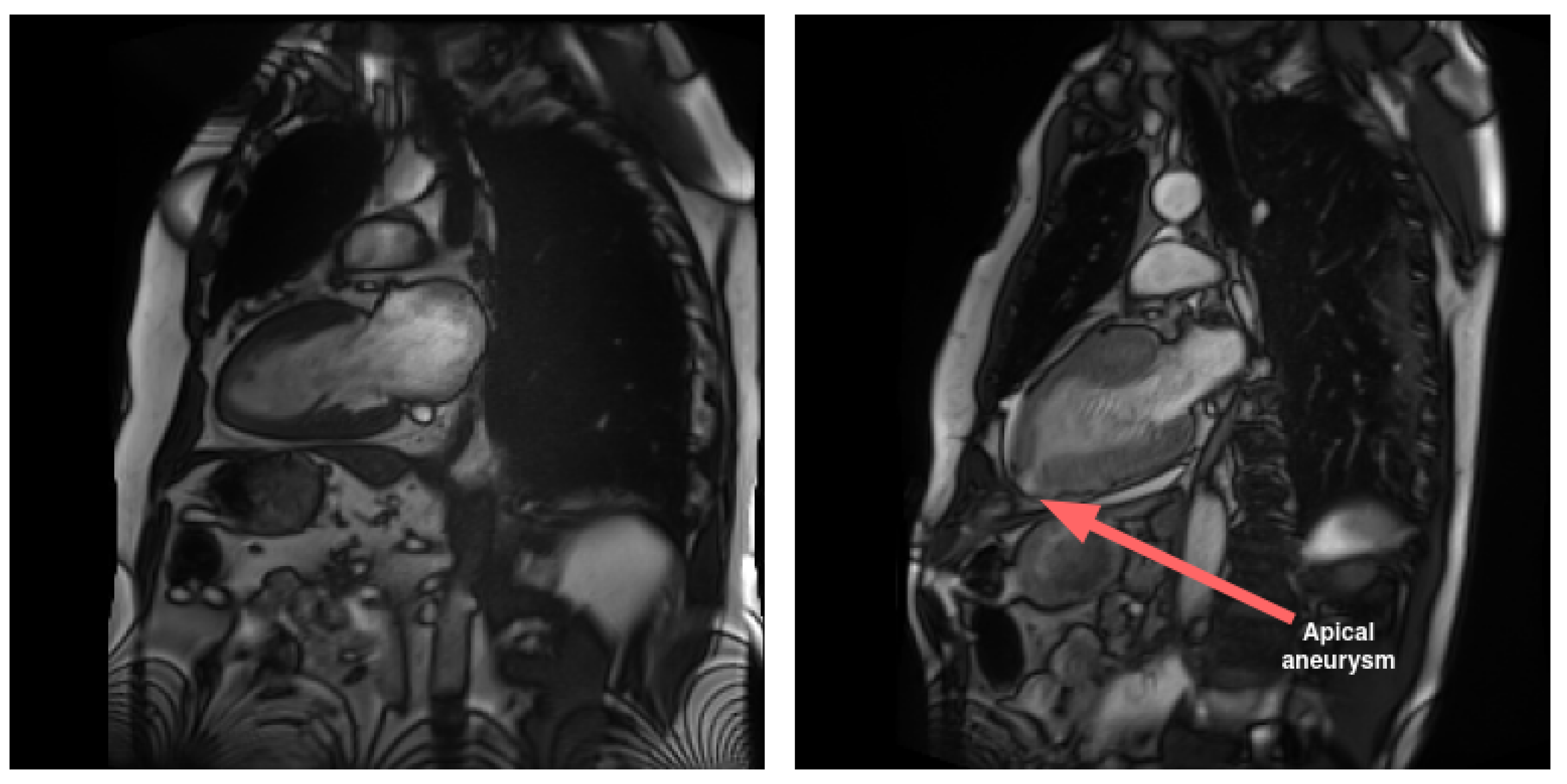
LAX views play a crucial role in imaging atria in comparison to SAX views. Specifically, LAX views are instrumental in visualizing pathological conditions that impact this area of the heart, such as malformations and interatrial communications. Additionally, LAX views contribute to the diagnosis of diseases affecting the apical region of the heart. In contrast to the SAX view, the LAX view enables the assessment of the apical region, as illustrated in Figure 1.

While segmentation for CMRI is a well-investigated domain, the majority of studies predominantly concentrate on SAX segmentation [5], with a particular emphasis on utilizing Cine-MRI sequences. Conversely, LAX views have received comparatively less attention, with methods developed for other image orientations, particularly in SAX [6,7,8,9,10,11,12].

Few studies have conducted an in-depth examination of Cine-MRI long-axis cardiac images, as exemplified by the $\Omega$-net method proposed by Vigneault et al. [13]. In this work, the authors addressed multiclass segmentation for SAX, LAX two-chamber and four-chamber views by employing a predelineation UNet. The bottom features from this UNet were utilized to train a Spatial Transformer Network [14], allowing the learning and estimation of rigid affine transformation matrix parameters to achieve a canonical orientation consistent with clinical practices across the dataset. Following this transformation, the output was directed to a second segmentation pipeline comprising multiple chained UNets. For LAX four-chamber images, the authors annotated over five classes in addition to the background class, facilitating whole-heart segmentation. This study involved full cardiac cycle annotation. The reported results include average Intersection over Union (IoU) scores of 0.856 and 0.845 for LAX two-chamber and LAX four-chamber, respectively.

Another study involving fully annotated LAX four-chamber was conducted by Bai et al. [15]. In this work, the authors compared a semisupervised learning pipeline to a baseline UNet by using a small amount of annotated data. They reached average respective Dice scores of 0.934 ± 0.029 and 0.930 ± 0.032 by using 200 training slices corresponding to ED and ES timeframes for 100 examinations. Their approach introduces a distinct starting postulate, considering the various axes of view as entangled. The idea is that these axes can be learned through shared anatomical features at their intersections, thereby enhancing segmentation by incorporating surrounding features. The most promising outcomes were attained by employing a multitask pipeline that simultaneously addressed both anatomical intersection detection and segmentation.

In previous work, Bai et al. [16] used a VGG16 [17] architecture to automatically segment atria from LAX four- and two-chamber Cine-MRI images. They attained respective Dice scores of 0.93 ± 0.05 on the LAX two-chamber left atrium and 0.95 ± 0.02 and 0.96 ± 0.02 for the LAX four-chamber left atrium and right atrium, respectively. It is worth mentioning that they achieved inference times of approximately 0.2 s for the ED and ES LAX images and 1.4 s when the entire sequence was included.

Other notable works involve the integration of Statistical Models of Deformation (SMOD) with UNet-based segmentation, as proposed by Acero et al. [18]. Their study focused on hypertrophic cardiomyopathy and normal examinations, incorporating LAX two- and four-chamber views, with the right atrium being the sole missing class. Al Khalil et al. [19] used SPADE-GAN image generation in conjunction with VAE-based label deformation by interpolation over LAX four-chamber images to perform data augmentation prior to segmentation. The augmentation generated by the GAN improved their results compared to the use of more traditional morphological alterations [20]. Additionally, Pei et al. [21] and Wang et al. [22] utilized images from the LAX four-chamber view to implement domain adaptation with feature differentiation between CT and MR modalities. The M&M2 challenge incorporated images from the LAX four-chamber view as part of the segmentation task, with a specific focus on right ventricle segmentation [23]. Various methods were developed by participants, employing the four-chamber view in independent pipelines [6,7,8] or through shared information pipelines, with LAX data often utilized to refine SAX segmentation [9,10,11,12]. Notably, among the top-performing methods for the LAX four-chamber segmentation task, excluding the approach proposed by Li et al. [9], separate pipelines were employed, with no information sharing between SAX and LAX.

Most other works have primarily focused on LAX segmentation targeting one or two anatomical structures. These encompass various deep learning approaches [24,25,26] or hybrid pipelines combining deep learning, as exemplified by Zhang et al. [27]. Additionally, Sinclair et al. [25] and Leng et al. [26] also included the LAX three-chamber view, an orientation that is less often studied in segmentation tasks compared to LAX two-chamber and four-chamber views. Notably, Gonzales et al. [28] introduced an automated left atrium segmentation method utilizing active contours on a polar grid. Their approach involves employing a residual network for extracting mitral-valve-insertion points in a preprocessing step. Subsequently, edge reconstruction and Cartesian mapping are applied to obtain the final segmentation.

Over recent years, several deep learning architectures have been applied to tasks related to medical-imaging segmentation. The most notable, UNet, introduced by Ronneberger et al. [29], has been used in numerous works, with various adaptations and modifications [30,31]. This architecture and its derived variants have consistently achieved state-of-the-art performances when applied to medical-image segmentation [23,32]. Additionally, both prior to and concurrently with UNet, Fully Convolutional Networks (FCNs) have also been employed, yielding acceptable results [16].

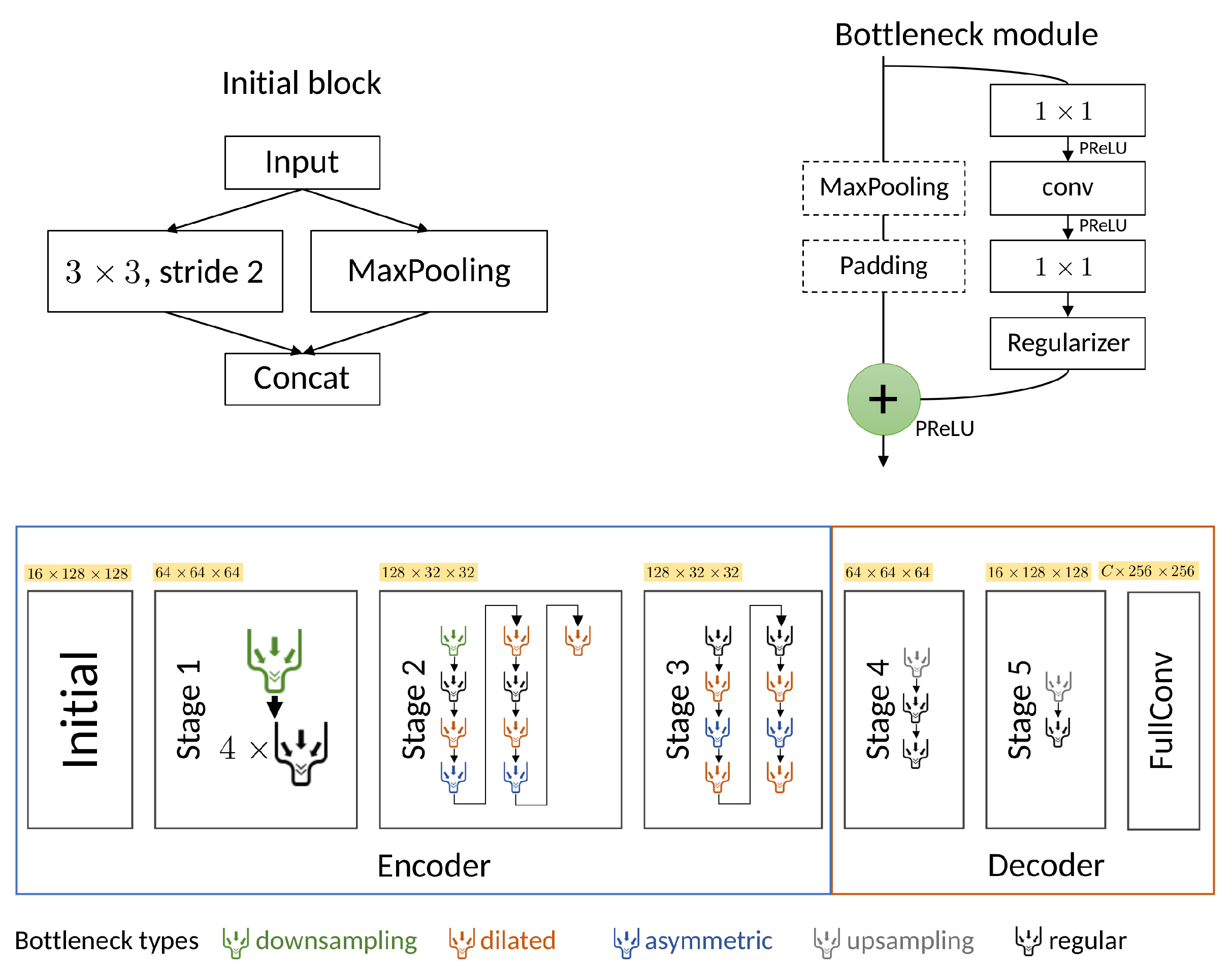
We employed the ENet architecture by Paszke et al. [33] due to its capability to produce effective segmentation results with lower computational costs and faster inference. A detailed description of the architecture is provided in Section 2.2. The ENet architecture has previously found application in the medical-imaging domain [34,35,36,37]. For instance, Salvaggio et al. achieved favorable results in prostate-volume estimation by using ENet [34]. Furthermore, Karimov et al. conducted a performance evaluation of ENet, comparing it against UNet by using histological slices [37]. Their findings indicated that ENet achieved a Dice performance comparable to UNet but demonstrated a superior computational efficiency, with performance gains of up to 15 times.

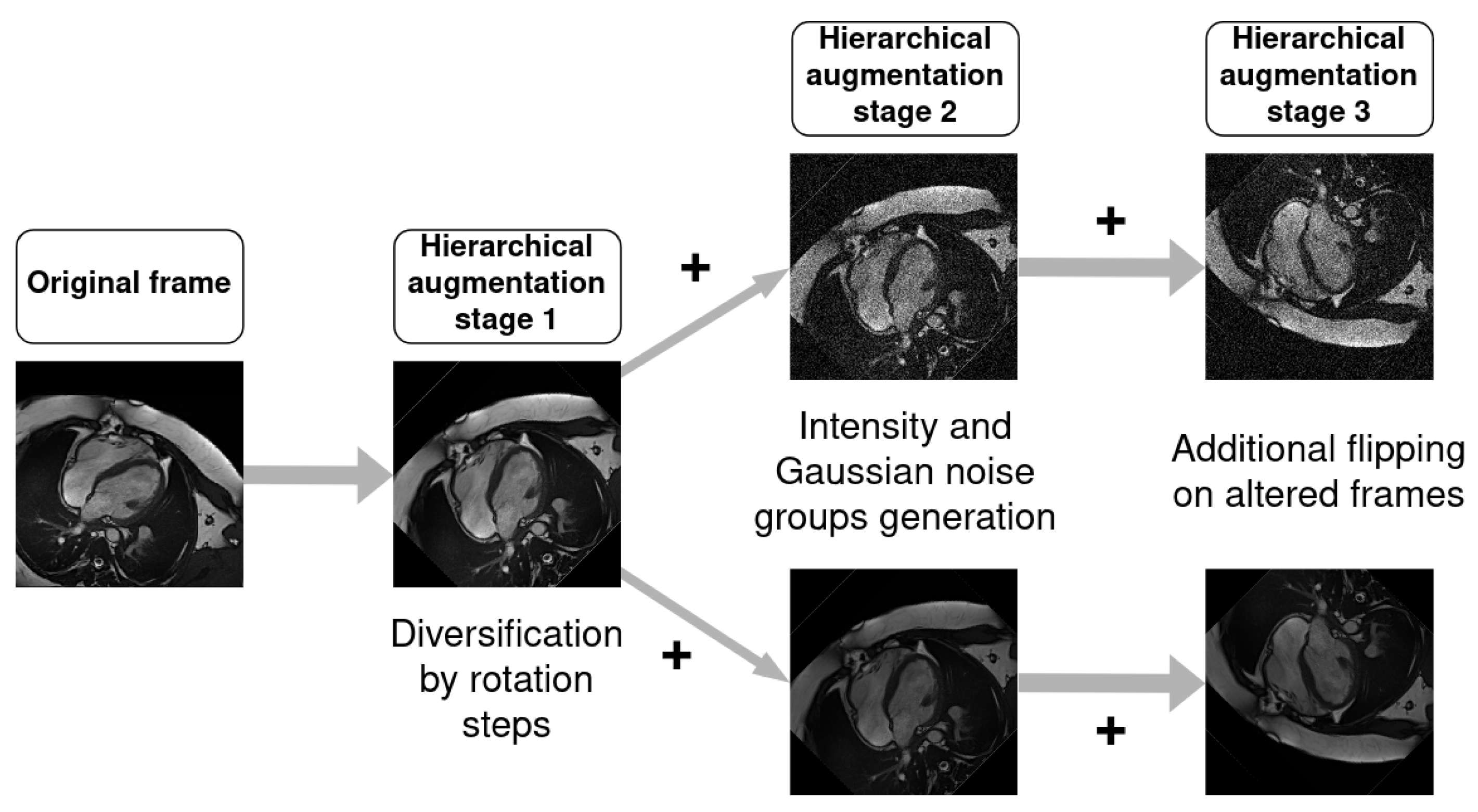
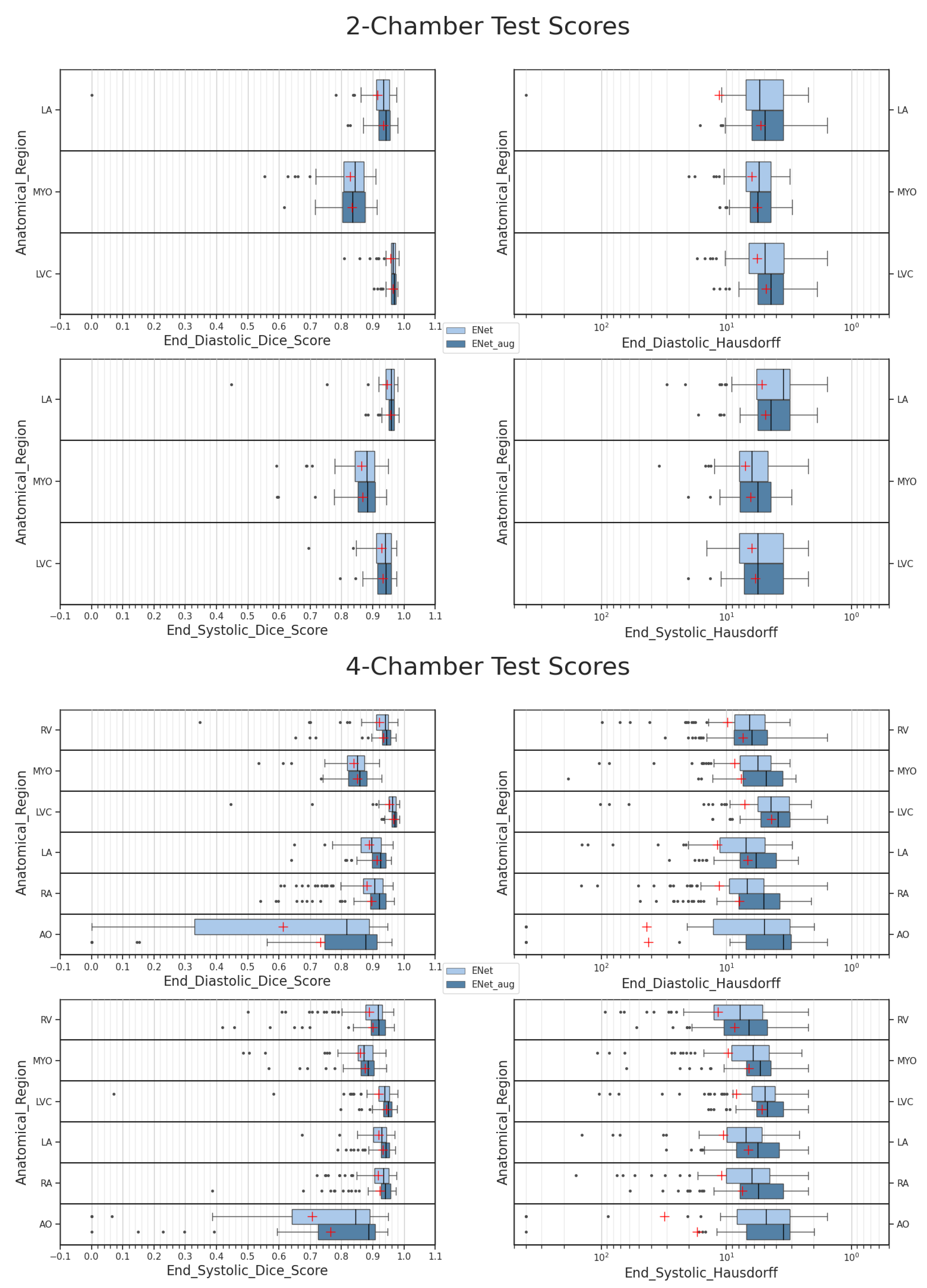
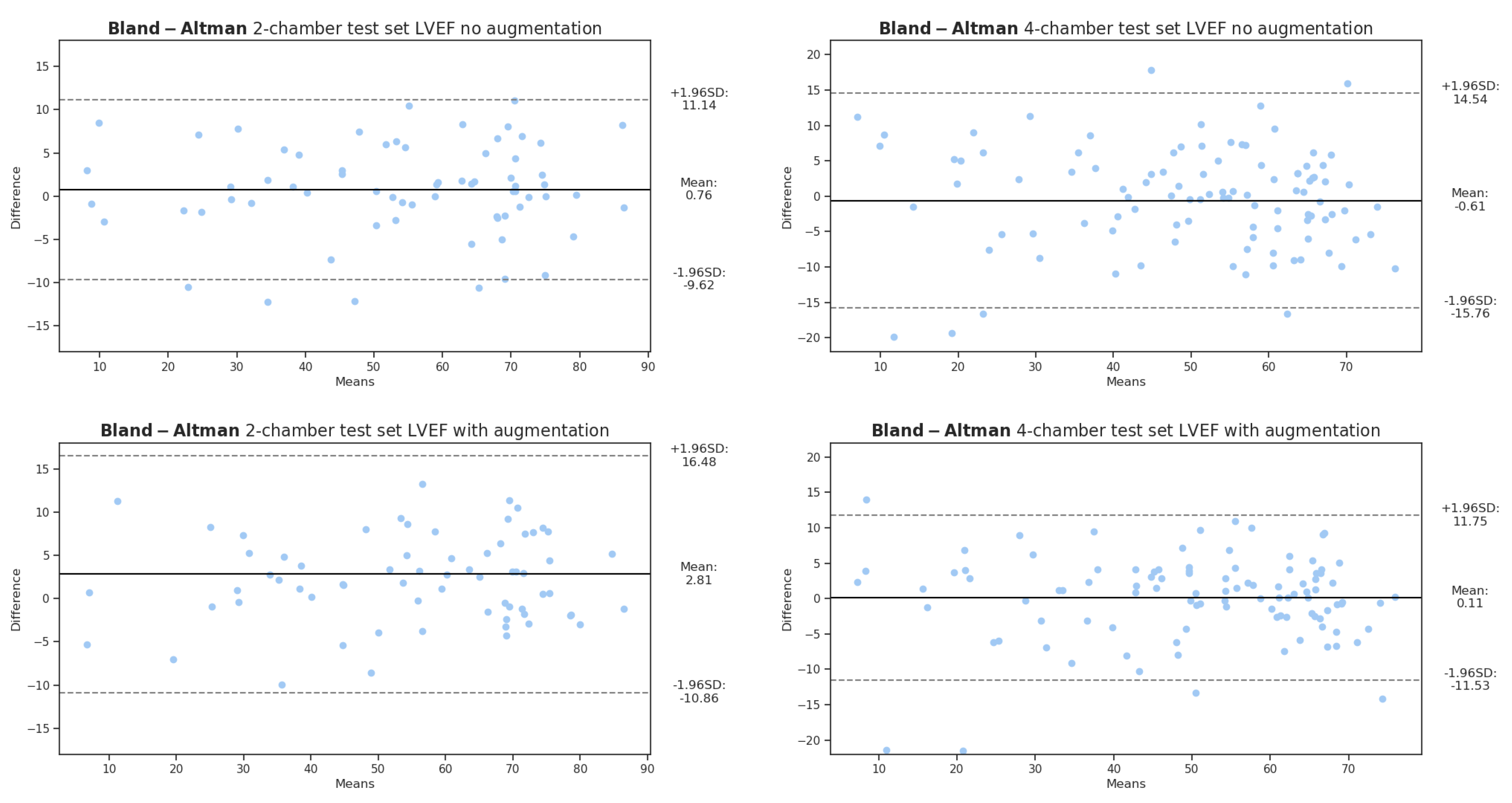
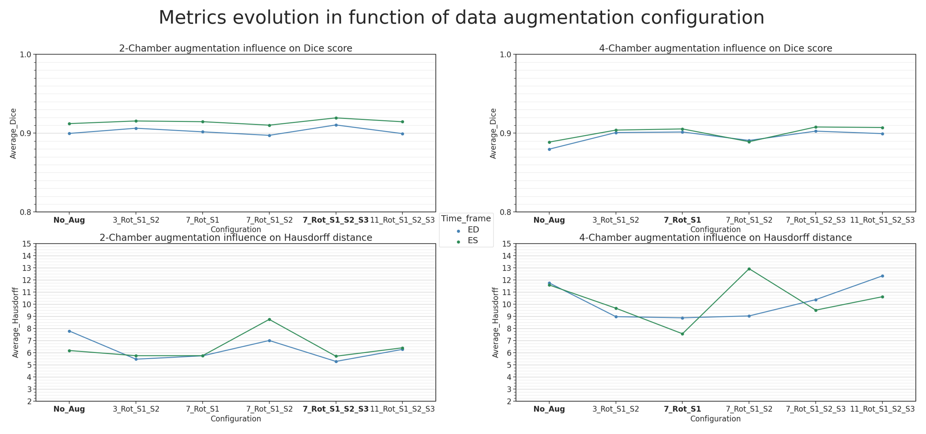
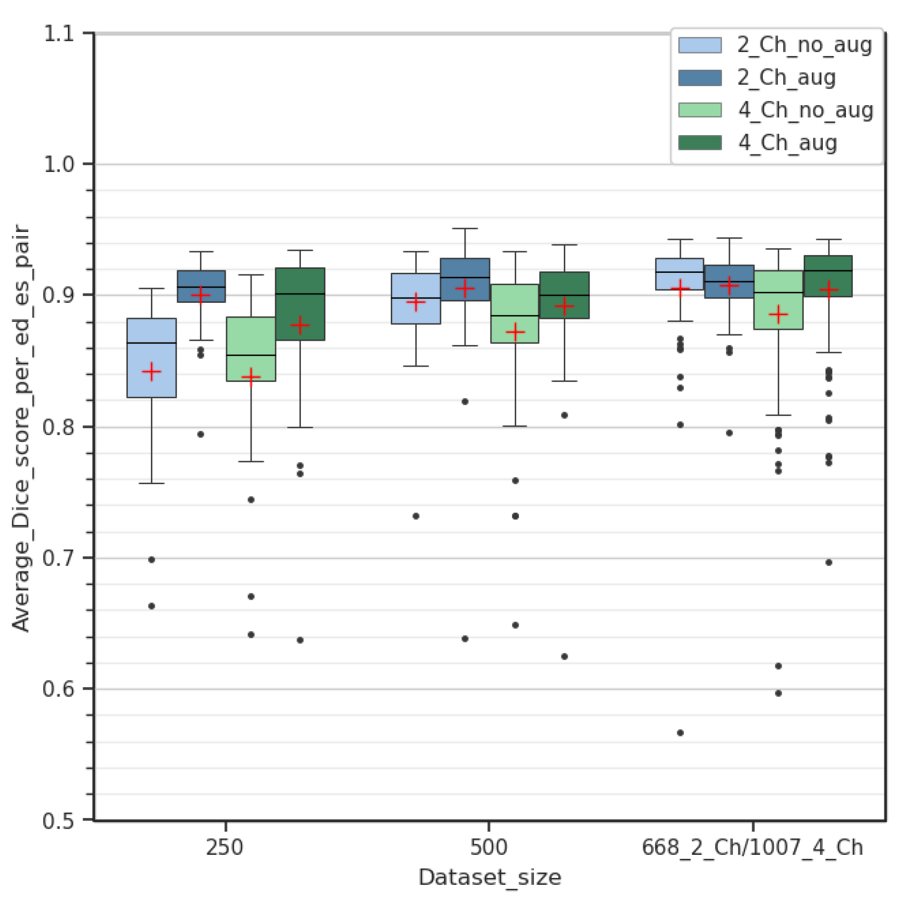
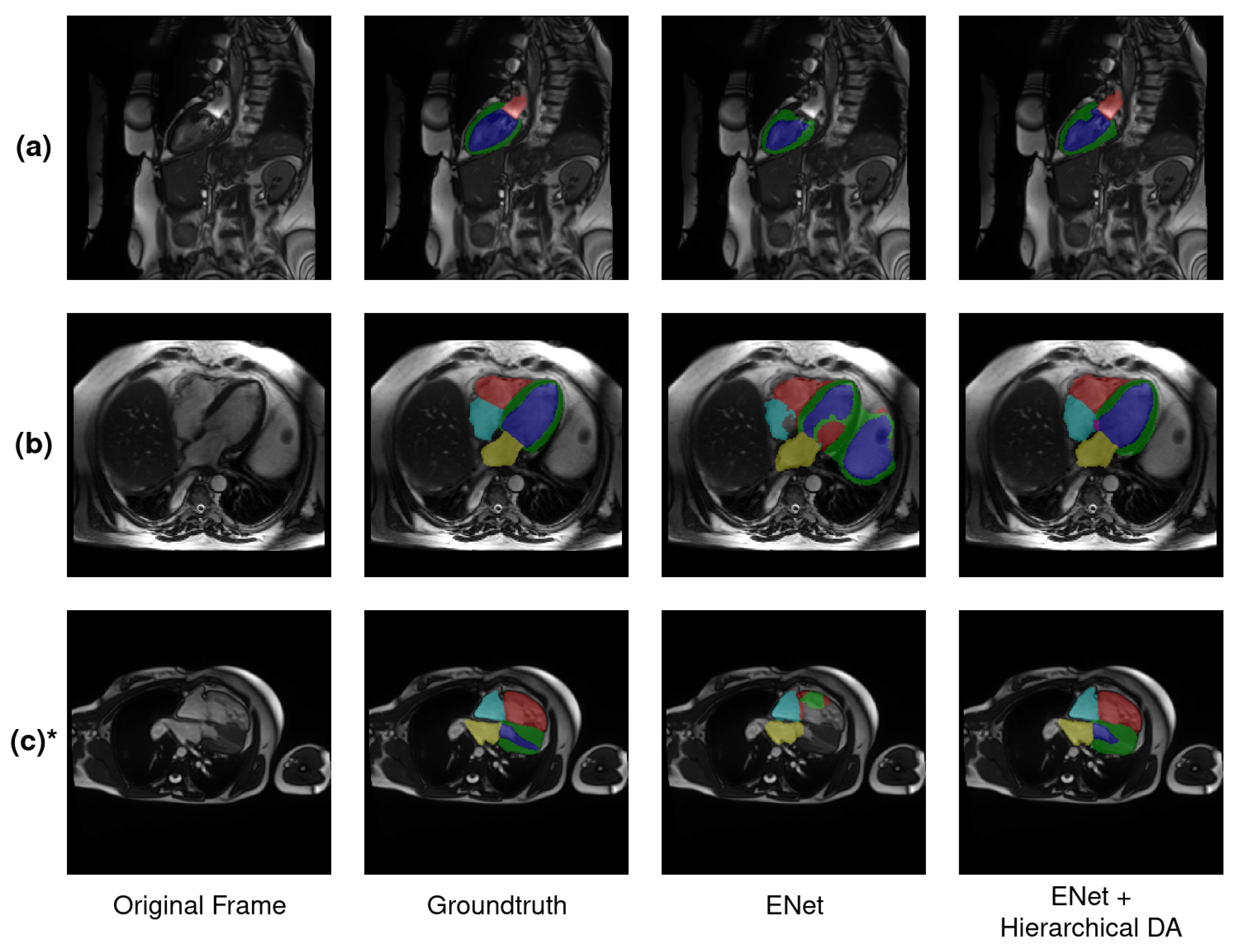
In the realm of cardiac Cine-MRI segmentation, ENet has primarily been utilized for SAX when applied to the MRI modality [35,36]. To the best of our knowledge, our study represents the first instance of using the ENet architecture for long-axis two- and four-chamber segmentation in Cine-MRI. In contrast to the previously mentioned works, the current article concentrates on whole-heart segmentation in both LAX two- and four-chamber views and does not involve a SAX study. Our assessment specifically explores the impact of hierarchical data augmentation on segmentation improvement, with an additional focus on extrapolating the Left Ventricular Ejection Fraction (LVEF).

The remainder of this paper is structured as follows. In Section 2, we provide details on the datasets, our hierarchical data-augmentation technique and the network architecture used for our comparison. In Section 3, the scores with and without data augmentation are presented as well as the clinical metric estimation over the LVEF. In Section 4, the segmentation results are analyzed along the data-augmentation influence, and finally, in Section 6, we present our conclusions.

2. Materials and Methods

The proposed pipeline targets whole-heart segmentation over LAX 2- and 4-chamber Cine-MRI images. The objective is to automatically produce anatomically accurate segmentation maps from original image acquisition. The procedure is carried out through the use of an ENet model trained on an augmented dataset with transforms and alterations following a hierarchy-based protocol. A practical usage demonstration is shown in Section 3.3.

2.1. Datasets

2.1.1. Annotation Rules

For training the models, two datasets containing Cine-MRI LAX 2-chamber and 4-chamber images were utilized, comprising 668 and 1007 examinations, respectively. The variation in the dataset sizes is partially attributed to the nonavailability of anatomical ground truths for some examinations. For each Cine-MRI study, end-diastolic (ED) and end-systolic (ES) phases of the cardiac cycle were visually selected and annotated under the supervision of an expert physicist. The segmentation task in the 2-chamber view focused on the left ventricle cavity (LVC), the myocardium (MYO) and the cavity of the left atrium (LA). For the 4-chamber view, three additional classes were used: the cavities of the right ventricle (RV) and the right atrium (RA), along with the aortic root (AO). The aortic root class was introduced to address cases where the aorta is visible on the image in a 4-chamber orientation. The absence of a consistently present aortic root class across all samples contributes to the segmentation complexity in the 4-chamber view.

In both orientations, specific rules based on anatomy were established. The LVC must be disconnected from the background and enveloped by the MYO class. Additionally, the LVC must also be in direct contact with the LA at the level of the atrioventricular valve. If present, the AO class must also be in direct contact with the left ventricle cavity at the level of the aortic valve.

2.1.2. Database Information

The majority of the examinations were retrieved and anonymized from CHU-Dijon Hospital. The acquisitions were performed by using the AERA, SOLA and SKYRA scanner models from Siemens. Notably, the SKYRA model has a 3.0 Tesla field strength, while the other scanners operate at 1.5 Tesla. In both LAX orientations, an additional subset of 44 examinations from Siemens scanners, sourced from the DETERMINE LV Segmentation Challenge of the Cardiac Atlas Project validation database [38,39] was included. These examinations were conducted by using the AVANTO, SONATA and ESPREE scanner models.

For the LAX 4-chamber database, 219 examinations from the MnM2 challenge obtained by using Siemens scanners were also incorporated [23], thereby adding four additional sources to this database. The inclusion of MnM2 images contributes to the difference in the number of images between the two views, as mentioned in Section 2.1.1, given that the challenge did not specifically focus on the 2-chamber view. Existing annotations for examinations from these two additional sets were modified and adapted to the previously defined delineation procedures.

Image matrix sizes ranged from 156 × 192 to 290 × 352 voxels for 2-chamber images and from 192 × 156 to 352 × 330 voxels for 4-chamber images. The image resolutions are isotropic in the plane and range from 0.99 to 2.08 mm on both databases. The out-of-plane resolution varies from 1.00 to 9.00 mm on both databases. Since these sequences consist of a single spatial slice, the out-of-plane resolution was not considered for the experiments.

No selection based on pathology was made during the data collection. As a result, both datasets comprise multiple diseases in addition to normal examinations. The included conditions encompass myocardial infarction, cardiopathies and congenital conditions, many of which can potentially alter heart anatomy.

2.2. Network Architecture

In 2016, Paszke et al. introduced the Efficient Neural Network (ENet) for segmentation tasks [33], which is depicted in Figure 2. Despite sharing an encoder–decoder-based architecture with UNet, ENet exhibits significant differences. Notably, it features a small decoder, along with early and limited downsampling to preserve spatial fine-level features, serving as both an alternative and a complement to the skip-connections method. The ENet architecture is made up of six stages comprising an initial stage, followed by three stages forming the encoder and the last two stages forming the decoder.

The initial stage contains a single block shown at the top left of Figure 2. Stage 1 is composed of five bottleneck blocks while stages 2 and 3 share a similar structure, with the distinction that stage 3 lacks the downsample bottleneck. The different color-coded bottleneck modules correspond to a downsampling bottleneck, implemented by using a maxpooling parallel branch; the dilated, asymmetric or regular bottlenecks implemented by using corresponding convolutions; and the asymmetric bottleneck implemented by using a sequence of $5\times 1$ and $1\times 5$ convolutions. A detailed description of the architecture can be referred to in the original work [33].

The novelty of the ENet architecture lies in the various design choices made with a specific focus on improving the computational complexity. One such choice was the use of dilated convolutions and using saved indices from max pooling layers to produce sparse upsampled maps in the decoders. Other choices include the application of early downsampling to heavily reduce the input size, a smaller decoder size, using Parametric Rectified Linear Units (PReLU) instead of RELUs, implementing information-preserving dimensionality changes by performing pooling operations in parallel with a convolution of stride 2 and concatenating the resulting feature maps, among others.

The used ENet architecture in itself makes use of skip connections following the work of Lieman-Sifry et al. [35]. However, these connections are applied only over the maximum argument parameters extracted from early pooling layers and are passed to the unpooling layers of the decoder.

These strategies, among other minor tweaks, enable the architecture to learn with a wide reception field while keeping computational costs low. Despite the network’s structure comprising 358 different layers including 89 associated with convolutions, the amount of parameters remains low, totaling 0.373 M.

2.3. Methodology

2.3.1. Training Context

Each database was divided into training, validation and testing sets with respective proportions of $0.7$, $0.2$ and $0.1$. Prior to training, slices and labels were resized to 256 × 256 pixels, with in-plane isotropic pixel dimensions ranging from 0.99 to 1.95 mm in the LAX 2-chamber and from 0.99 to 2.08 mm in the LAX 4-chamber. In total, 135 and 68 examinations were used for validation and testing in the 2-chamber dataset, respectively, while the numbers reached 200 and 102 examinations for the 4-chamber dataset, respectively.

The training experiments were conducted over 100 epochs with data normalization applied during prior experiments. The Adam optimizer [40] was used to minimize a combination loss of equally represented multiclass cross-entropy and multiclass Dice. Class weighting was implemented to address the potential imbalance between the heart region and the surrounding areas. The class weights were determined based on the rules established in the work of Zotti et al. [41], with added emphasis on weakly represented classes such as AO. The experiments described in the presented work were performed on an NVIDIA RTX 4500 GPU, using the NVIDIA-Tensorflow 1.15.5 library.

2.3.2. Data Augmentation

Training was performed with and without data augmentation to observe the influence on the segmentation accuracy. The augmentation was performed following a hierarchical procedure as outlined in Figure 3, where original data were duplicated into multiple groups. Each group is associated with a specific image alteration and follows a set of predefined rotations.

The first stage comprised generating rotated versions of the input image r times, where $r\in \{3,7,11\}$ depending on the chosen configuration. The rotation angles took on values from the following sets:

$$\begin{array}{c}{R}_1\in \{-{30}^{\circ },0^{\circ },+{30}^{\circ }\}\\ R_2\in \{-{45}^{\circ },0^{\circ },+{45}^{\circ }\}\\ R_3\in \{-{60}^{\circ },-{45}^{\circ },-{15}^{\circ },0^{\circ },+{15}^{\circ },+{45}^{\circ },+{60}^{\circ }\}\\ R_4\in \{-{90}^{\circ },-{60}^{\circ },-{30}^{\circ },0^{\circ },+{30}^{\circ },+{60}^{\circ },+{90}^{\circ }\}\\ R_5\in \{-{90}^{\circ },-{75}^{\circ },-{60}^{\circ },-{45}^{\circ },-{15}^{\circ },0^{\circ },+{15}^{\circ },+{45}^{\circ },+{60}^{\circ },+{75}^{\circ },+{90}^{\circ }\}\end{array}$$

where $|R_1|=3$, $|R_2|=3$, $|R_3|=7$, $|R_4|=7$ and $|R_5|=11$. This resulted in $Nr$ images, where N is the total number of images in a given set.

The rotated images obtained from stage 1 were then subjected to alterations in the image intensity and noise during stage 2. An initial intensity normalizing augmentation was applied by scaling the pixel intensities with a uniformly sampled random value from the interval $[0.6,1]$. Subsequently, two parallel subgroups of images were generated. The first subgroup applied additive zero-mean Gaussian noise with a standard deviation uniformly sampled from the interval $[1\times {10}^3,5\times {10}^3]$. The second subgroup applied another intensity variation, this time uniformly sampled from the interval $[0.3,1]$.

The third stage comprised generating horizontally and vertically flipped versions of the already altered images from stage 2.

2.3.3. Metrics

The Dice coefficient (or Dice score) is a commonly used metric to assess semantic segmentation tasks. It enables the measurement of similarity between the obtained segmentation (prediction) and the ground truth. The coefficient is calculated by determining the ratio between the overlapping pixels and the total number of pixels from both the prediction and the ground truth. The Dice coefficient is computed using Equation (1):

$$Dice=\frac{2\times |Pred\cap Gt|}{\left|Pred\right|+\left|Gt\right|}$$

(1)

Dice coefficients have values between 0 and 1. A value of 1 indicates perfect similarity between the prediction and the ground truth, while a value of 0 means that the prediction is entirely different from the ground truth (no overlapping pixels). Predictions with higher accuracy approach Dice coefficients closer to 1.

In addition to the Dice coefficient, which assesses similarity globally, the Hausdorff distance is also used to gauge similarity locally. It involves measuring the maximum distance between the prediction and the ground truth. Spatial resolution must be taken into account for its calculation, as summarized by Equation (2):

$$d_H(P,G)=max[d_{PG},d_{GP}]=max\{\underset{p\in P}{max}[\underset{g\in G}{min}d(p,g)],\underset{g\in G}{max}[\underset{p\in P}{min}d(p,g)]\}$$

(2)

where lower values correspond to closer edges between prediction P and ground truth G, and therefore more accurate segmentations.

The left ventricular volume and ejection fraction are two of the most prominent clinical metrics used to assess segmentation methods. Several methods enable the extrapolation of these metrics by using the left ventricle segmentations obtained from LAX Cine-MRI images [42]. These methods can be applied to different modalities as long as the acquisitions share a similar plane of view and common anatomical features. For instance, the LVEF can be calculated by using the single-plane long-axis ellipsoid model, as was demonstrated by Bulwer et al. [42] on echocardiography images. The same method was used in this work to determine ED and ES volumes from ground truths and predictions, using Equation (3):

$$V=\frac{8}{3\pi }\times \frac{A^2}{L}$$

(3)

with A corresponding to the area of the left ventricle cavity region and L being the major axis. Postprocessing was performed before computing clinical metrics to prevent errors related to outlier detection. However, as depicted in Figure 4, the left ventricle cavity is often one of the easier classes for the models to segment.

3. Results

This section details the experiments conducted to characterize the differences in data augmentation between the two datasets. A comparison of the clinical metrics relative to the LVEF, as well as the ED and ES volumes between the ground truths and ENet outputs, is also presented. A total of 68 patient studies, each consisting of ED/ES image pairs, were used for the test set in the two-chamber dataset, while 102 studies were used for the four-chamber dataset.

3.1. General Observations

Better segmentation performances compared to four-chamber were achieved over the two-chamber dataset, both with and without hierarchical data augmentation. Mean Dice scores of 0.910 and 0.915 were achieved over the two- and four-chamber sets, respectively. The difference was more pronounced during the ES phase, with a Dice score of 0.919 on the two-chamber test set compared to 0.905 on the four-chamber test set. These results are not surprising as the two-chamber orientation contains fewer classes to segment and lesser anatomical shape variance compared to the four-chamber dataset. The difference in the amount of data available between the two sets is another factor that may affect the Dice score. Further experiments were carried out in Section 4.2 to investigate this aspect.

These factors make the two-chamber dataset easier to converge for the architecture, leaving a smaller margin of improvement that can be achieved with data augmentation. Concurrently, the Hausdorff distances were, on average, lower over the two-chamber orientation, on both the validation and test sets. A mean value of 5.49 mm over the two-chamber test was obtained, as shown in

Table 1. Average metrics scores at end-diastolic (ED) and end-systolic (ES) timeframes, with and without hierarchical data augmentation.

Models *	Dice						Hausdorff HD (mm)
	ED		ES		Mean Difference		ED		ES		Mean Difference
	DA	No DA	DA	No DA	Rel (%)	Abs (%)	DA	No DA	DA	No DA	HD (mm)	Abs (%)
ENet 2 cav test	0.910 ± 0.034	0.900 ± 0.072	0.919 ± 0.039	0.912 ± 0.059	0.85	0.99	5.28 ± 2.17	7.79 ± 17.98	5.71 ± 2.76	6.17 ± 3.87	1.49	21.35
ENet 2 cav val	0.903 ± 0.065	0.904 ± 0.055	0.916 ± 0.040	0.914 ± 0.042	0.05	0.06	5.90 ± 4.52	6.23 ± 5.24	6.14 ± 3.69	6.65 ± 5.08	0.42	6.52
ENet 4 cav test	0.902 ± 0.061	0.880 ± 0.080	0.905 ± 0.068	0.889 ± 0.082	1.90	2.15	8.87 ± 13.65	11.75 ± 21.51	7.56 ± 9.27	11.58 ± 20.63	3.45	29.58
ENet 4 cav val	0.906 ± 0.053	0.886 ± 0.084	0.907 ± 0.060	0.892 ± 0.082	1.75	2.02	7.33 ± 9.08	9.08 ± 15.14	8.45 ± 13.01	9.82 ± 16.37	1.56	16.51

with data augmentation. Comparatively, a mean value of 8.22 mm was obtained when computing the average of the ED and ES results over the data-augmented four-chamber set.

Performance differences between the ED and ES predictions are more pronounced in the two-chamber orientation, as observed in Table 1, especially regarding Dice scores. This difference is related to individual LA and MYO class performances, which show a marked increase in Dice at the ES phase, as can be seen in Figure 4. The difference is explainable by the larger size of these anatomical targets during end systole, making them easier to segment. On the contrary, differences between the average Dice at ED and ES are less pronounced with the four-chamber test set. As can be observed from Figure 4, this is related to the greater amount of anatomical regions with divergent behaviors, leading to a homogenization of the Dice performance between ED and ES, as shown in Table 1.

The significant variation and lower performance over AO in the four-chamber set can be explained by its lower presence in the dataset. Moreover, this anatomical region presents variations among subjects, and its occurrence depends on the spatial orientation chosen during the acquisition (Table 5).

3.2. Influence of Data Augmentation

Both architectures were trained on augmented datasets following procedures described previously in Section 2.3.2. Using this hierarchical strategy, several configurations were tested, involving varying degrees of rotation applied to all of the generated groups of normal and altered images. In the lightest configuration, only rotation-based data augmentation was performed by using $R_3$, including rotations ranging from −60° to +60° over seven steps, along with the preliminary intensity alteration. This experiment is denoted as ENet + Stage 1 Aug in Table 4 and 7_Rot_S1 in Figure 7, respectively.

The heaviest configurations involved all three hierarchical stages of augmentation. The corresponding experiments are later referred to as ENet + FullAug 11 rotation steps and ENet + FullAug in Section 4.2 and are associated with 11_Rot_S1_S2_S3 and 7_Rot_S1_S2_S3 in Figure 7, respectively.

In some intermediate augmentation configurations, the third stage was removed. Instead, an additional frame-alteration group focused solely on image flipping is placed in the second stage. This augmentation was performed in parallel with the image-quality-alteration groups instead of being applied to them sequentially, making it mostly geometric in nature. The number of rotations was also reduced to mitigate the overfitting issues arising from data similarity. With the lightest of these intermediate configurations, the rotation configurations $R_1$ and $R_2$ were used, with $r=3$ rotations. The experiments involving two-stage augmentation are referred to as ENet + Stages 1 and 2 Aug and ENet + Stages 1 and 2 Aug 3 Rotation Steps in Section 4.2. They correspond to the labels 7_Rot_S1_S2 and 3_Rot_S1_S2 in Figure 7, respectively.

Using the heaviest data-augmentation process, 51,150 and 77,550 training images were generated from the two- and four-chamber datasets, respectively, compared to 930 and 1410 with no data augmentation. While most of the configurations referred above were shared between databases, the rotation range was settled at a wider amplitude of 45° for the four-chamber dataset compared to the 30° two-chamber dataset in configuration Stages 1 and 2 Aug 3 Rotation Steps. This change was made as acquisitions showed more anatomical variation over the four-chamber dataset, as seen in Figure 9c, for example. In general, data augmentation proved to be beneficial across the two orientations, although with different best-performing configurations. The experiments ENet + Stage 1 Aug and ENet + FullAug were associated with the best metric results over the four-chamber and two-chamber sets, respectively. Their corresponding results are reported in Table 1, Tables 4 and 6.

More-robust metric scores were observed across all classes, as seen in Figure 4. The average markers in red show a general increase in Dice on both the ED and ES frames. Moreover, the computed Hausdorff scores display a general decrease in correlation as the Dice increases. The performance improvement is more visible over the four-chamber dataset, with higher differences in the Dice and Hausdorff scores, as can be inferred from Table 1. On the other hand, this increase is less significant for the two-chamber dataset, with a less consistent difference. This behavior is not surprising, in part due to the segmentation task being easier due to a lower number of classes and the segmentation performances already being convincing without data augmentation. Details regarding the latter observation are provided in Section 4.2.

With both datasets, the Dice score and Hausdorff distance show a reduction in the amount of outliers and in the standard deviation for both the ED and ES phase when data augmentation is applied.

3.3. Clinical Metrics

The Dice score and Hausdorff distance were estimated on both validation and test sets, as reported in Table 1, Tables 4 and 6. Following the same rule, clinical metrics were computed with respect to the ground truths. The results of the ED and ES volumes and Left Ventricular Ejection Fraction (LVEF) are reported in

Table 2. Average left ventricular clinical metrics obtained with augmented and nonaugmented configurations. The ground-truth values from manual annotations are shown in parentheses.

Models	Average ED Volume (mL)		Average ES Volume (mL)		LVEF (%)
	DA (gt)	No DA (gt)	DA (gt)	No DA (gt)	DA (gt)	No DA (gt)
ENet 2 cav test	180 ± 67 (181 ± 70)	177 ± 69 (181 ± 70)	85 ± 71 (91 ± 72)	88 ± 71 (91 ± 72)	56.65 ± 19.70 (53.84 ± 19.97)	54.60 ± 20.15 (53.84 ± 19.97)
ENet 2 cav val	177 ± 70 (179 ± 71)	177 ± 68 (179 ± 71)	86 ± 64 (88 ± 66)	87 ± 63 (88 ± 66)	55.31 ± 18.06 (55.12 ± 17.33)	54.53 ± 18.14 (55.12 ± 17.33)
ENet 4 cav test	152 ± 59 (157 ± 59)	155 ± 72 (157 ± 59)	79 ± 53 (83 ± 57)	82 ± 58 (83 ± 57)	50.32 ± 17.62 (50.21 ± 17.57)	49.60 ± 17.66 (50.21 ± 17.57)
ENet 4 cav val	146 ± 58 (151 ± 61)	142 ± 57 (151 ± 61)	74 ± 51 (80 ± 52)	73 ± 49 (80 ± 52)	53.43 ± 15.51 (51.42 ± 14.74)	51.82 ± 14.99 (51.42 ± 14.74)

. The ED and ES volumes were approximated following the method described in Section 2.3.3. The average results of the validation and test sets are presented in Table 2.

The computed ED and ES volumes are generally close to the values obtained from the ground truths. However, a small negative bias can be observed both over the ED and ES frames. The volumes from automatic processing are, on average, systematically lower compared to the given ground-truth values. The LVEF percentages show a small overestimation with selected models from data augmentation.

We observed that with the four-chamber dataset, an increase in Dice by 2% was correlated with an improvement in the LVEF metric from a mean bias of −0.61 to +0.11, as seen in Figure 5. Conversely, for the two-chamber dataset, an increase of 0.75% in Dice was associated with a deterioration in the mean bias from +0.76 to +2.81%. This decrease in performance could be related to the difference in the location of the mitral valve boundary between ground truths and predictions. Comparatively, the agreement is better with the four-chamber dataset, on both the augmented and nonaugmented configurations. Another possible reason resides in the smaller set size of the two-chamber orientation, rendering it more responsive to outliers.

Lower LVEF differences were obtained over the validation sets, as reported in Table 2. This can be attributed to the higher number of examinations available compared to the test set, resulting in a finer representation of the encountered anatomical variations.

4. Discussion

This section presents the results of the experiments, with a specific focus on the effect of data augmentation. Before delving into the effects of data augmentation, the results of K-fold cross-validation are presented to demonstrate the consistency of the models and the training procedure.

4.1. K-Fold Cross Validation

To evaluate the robustness of the architecture, a K-fold cross-validation was conducted on both original datasets without augmentation, with $K=5$. For each fold, 10% of the dataset was set aside for testing to ensure that the test size remained constant across all of the experiments. The original random seed was fixed to guarantee consistent testing throughout. In total, 600 and 905 examinations were utilized for cross-validation inference for the two- and four-chamber datasets, respectively. A second randomization seed was fixed to ensure consistent shuffling in the training set. The results for the Dice score and Hausdorff distance are reported in

Table 3. Average Dice (DSC) and Hausdorff (HD) scores across the K folds of cross-validation. Experiments were applied to nonaugmented datasets.

Models	K1		K2		K3		K4		K5
	Mean DSC	Mean HD	Mean DSC	Mean HD	Mean DSC	Mean HD	Mean DSC	Mean HD	Mean DSC	Mean HD
ENet 2 cav	0.897	6.66	0.905	6.18	0.905	6.39	0.903	8.27	0.897	7.00
UNet 2 cav	0.896	13.31	0.896	14.00	0.892	17.05	0.894	8.83	0.891	9.54
ENet 4 cav	0.886	13.73	0.880	12.55	0.885	13.20	0.889	10.34	0.883	13.87
UNet 4 cav	0.904	11.88	0.906	12.18	0.905	9.46	0.903	9.85	0.910	10.96

and Figure 6.

The Hausdorff distance exhibited higher variability due to its sensitivity to localized outliers in predictions. Dice coefficient differences remained low across folds, indicating consistent model learning. Any discrepancies compared to the reported results in Table 1 and

Table 4. Representative scores of the tested data-augmentation configurations. Model experiences in bold are those retained for computed augmentation metrics in Table 1 and Table 2. When not indicated, 7 rotation steps were applied by default, as shown in Figure 7.

2-Chamber Models	Validation Set (135 Examinations)				Test Set (68 Examinations)
	End Diastole		End Systole		End Diastole		End Systole
	Dice	Hausdorff(mm)	Dice	Hausdorff(mm)	Dice	Hausdorff(mm)	Dice	Hausdorff(mm)
ENet NoAug	0.904 ± 0.055	6.23 ± 5.24	0.914 ± 0.042	6.65 ± 5.08	0.900 ± 0.072	7.79 ± 17.98	0.912 ± 0.059	6.17 ± 3.87
ENet + Stage 1 Aug	0.899 ± 0.057	5.96 ± 4.25	0.914 ± 0.038	6.09 ± 3.70	0.902 ± 0.037	5.74 ± 2.47	0.915 ± 0.038	5.75 ± 2.70
ENet + Stages 1 and 2 Aug 3 Rotation Steps	0.900 ± 0.056	6.25 ± 5.13	0.915 ± 0.039	6.41 ± 4.20	0.906 ± 0.039	5.46 ± 2.41	0.916 ± 0.039	5.75 ± 2.59
ENet + Stages 1 and 2 Aug	0.891 ± 0.067	7.92 ± 17.35	0.911 ± 0.041	6.73 ± 4.16	0.897 ± 0.047	7.00 ± 10.17	0.910 ± 0.045	8.74 ± 16.25
ENet + FullAug 11 Rotation Steps	0.894 ± 0.069	7.30 ± 14.28	0.914 ± 0.041	6.33 ± 4.50	0.899 ± 0.040	6.27 ± 6.35	0.915 ± 0.037	6.40 ± 5.77
ENet + FullAug	0.903 ± 0.065	5.90 ± 4.52	0.916 ± 0.040	6.14 ± 3.69	0.910 ± 0.034	5.28 ± 2.17	0.919 ± 0.039	5.71 ± 2.76
4-Chamber Models	Validation Set (200 Examinations)				Test Set (102 Examinations)
	End Diastole		End Systole		End Diastole		End Systole
	Dice	Hausdorff (mm)	Dice	Hausdorff (mm)	Dice	Hausdorff (mm)	Dice	Hausdorff (mm)
ENet NoAug	0.886 ± 0.084	9.08 ± 15.14	0.892 ± 0.082	9.82 ± 16.37	0.880 ± 0.080	11.75 ± 21.51	0.889 ± 0.082	11.58 ± 20.63
ENet + Stage 1 Aug	0.906 ± 0.053	7.33 ± 9.08	0.907 ± 0.060	8.45 ± 13.01	0.902 ± 0.061	8.87 ± 13.65	0.905 ± 0.068	7.56 ± 9.27
ENet + Stages 1 and 2 Aug 3 Rotation Steps	0.902 ± 0.064	7.65 ± 8.93	0.904 ± 0.064	8.40 ± 11.84	0.901 ± 0.059	8.97 ± 10.93	0.903 ± 0.065	9.83 ± 15.03
ENet + Stages 1 and 2 Aug	0.891 ± 0.067	8.82 ± 12.45	0.895 ± 0.067	9.16 ± 16.61	0.891 ± 0.066	9.03 ± 15.30	0.888 ± 0.075	13.11 ± 23.63
ENet + FullAug 11 Rotation Steps	0.903 ± 0.063	9.19 ± 15.96	0.905 ± 0.066	10.11 ± 17.03	0.899 ± 0.061	12.33 ± 21.57	0.907 ± 0.065	10.72 ± 19.94
ENet + FullAug	0.903 ± 0.063	8.25 ± 17.26	0.907 ± 0.064	8.99 ± 13.04	0.903 ± 0.060	10.37 ± 15.88	0.907 ± 0.060	9.66 ± 14.72

can be attributed to the training variability.

4.2. Differences in Data Augmentation

As mentioned in Section 2.3, several augmentation configurations were implemented with varying degrees of rotation, flipping and the inclusion or exclusion of image-quality alterations through noise and intensity variations. Different behaviors were observed for each dataset. From Table 4 and Figure 7, it is evident that the best performances are achieved with the ENet architecture trained on the two-chamber augmented dataset generated for the ENet + FullAug configuration. This configuration corresponds to the full hierarchical pipeline data augmentation schematized in Figure 3. The primary contributing factor here was the number of generated rotation steps, as an excessive number of rotations led to lower performances, as was seen with the ENet + FullAug 11 Rotation Steps configuration. The ENet + FullAug configuration, comprising seven rotation steps, yielded the best results.

Apart from rotation, the strategy used for flipping plays an equally important role in improving the segmentation. This was observed in the augmentation configuration with two stages. In this case, flipping as a separate processing group in parallel to image alterations may contribute to decreased performances, as opposed to being applied in the third stage. This is particularly more visible with the ENet + Stages 1 and 2 Aug configuration, which also used seven rotation steps. Lowering the number of rotations in the ENet + Stages 1 and 2 Aug 3 Rotation Steps configuration improved metrics in both cases, although not up to the best-achieved results.

On the other hand, experiments using data augmentation solely based on rotations with moderate intensity changes led to the best results achieved with the four-chamber dataset. While the average results are lower than those obtained in the two-chamber dataset, the improvements tend to be more pronounced in comparison. With the exception of the aforementioned ENet + Stages 1 and 2 Aug configuration, a clear increase is observed over the Dice metric with all augmentation configurations tried on the four-chamber dataset. This difference between the results with both augmented datasets can be attributed to the higher variability of the encountered situations present in the four-chamber dataset, leading to more configurations with potential image-quality variations. Overall, this point supports the conclusions shared by Martin-Isla et al. [23] and Beetz et al. [43], where a mix of both shape modification and image-quality alterations led to improved segmentation. Another factor contributing to the observed difference in improvement is the presence of difficult segmentation classes with more complex forms, as well as the inconsistently present AO class.

Further experimentation was carried out by comparing the average Dice improvement between different dataset configurations, as shown in Figure 8. Random examinations were chosen to generate smaller datasets, comprising 250 and 500 ED/ES image pairs, respectively, for both two-chamber and four-chamber views. The corresponding test sets contained 25 and 50 examinations/pairs, respectively. For this experiment, the ENet + Stage 1 Aug configuration was applied to both views.

Data augmentation demonstrated a more pronounced Dice improvement over the two-chamber dataset with a limited amount of data. However, as the number of examinations increased, this improvement became less noticeable, contrary to what can be inferred with the four-chamber dataset in Figure 8. While the quantity of examinations differs between datasets for reasons provided in Section 2.1, this additional experiment demonstrates that it is plausible to expect a similar trend if the number of examinations was the same across both datasets.

4.3. Handling of Difficult Examinations

Gathering data from different sources with no pathological filtering can introduce difficult cases that, although uncommon, are susceptible to being encountered in clinical practice. Several factors contribute to the complexity of analyzing an examination. The first one is anatomical and/or pathological, especially with deformed hearts, as seen in conditions such as the tetralogy of Fallot, dilated right ventricle or aneurysm. A second factor resulting in challenging cases stems from image-quality degradation. These alterations result from various causes such as field inhomogeneities, noise and artifacts related to motion, partial volume effects or cardiac implants. These two factors affect myocardium delineation, as observed in Figure 9a,c, in the case of artifacts or severe anatomical deformation.

A third factor is related to the choice of the slice axis plane, as it may influence the potential occurrences of visible anatomical regions to be detected. This is especially true with the aortic root in the four-chamber orientation, as its presence depends on the plane chosen during acquisition. Pertaining to these aspects, our hierarchical data augmentation plays a crucial step in reducing potential detection errors related to the first two factors mentioned (Figure 7).

It is worth mentioning that in these examples, a region corresponding to the aortic root was falsely segmented with data augmentation, even when it was not present in the original ground truth in Figure 9b. This can be explained by the difficulty for the network to determine a clear boundary feature for this anatomical region, which is both induced by its nonsystematic presence across the frames as well as the significant anatomical changes in the images between subjects and between the end-diastole and end-systole phases. These challenges came into play with the computed performance, resulting in lower metrics and a higher rate of failures in this class compared to other regions. Nevertheless, in the above example, the model produced a noncorrect but visually plausible segmentation map with respect to these points.

For the current experiments, the aortic root was segmented to reduce the gap that was sometimes present between atria and as an attempt to mitigate associated segmentation errors. Sensitivity and specificity were also computed for this segmentation class in

Table 5. True positive and true negative rates on aortic root segmentation at end-diastole ED and end-systole ES, computed after selected 4-chamber data-augmentation training.

Aorta-Detection Metrics	Validation Set (200 Examinations)		Test Set (102 Examinations)
	ED	ES	ED	ES
True positive	41	42	29	33
True negative	143	134	65	64
False positive	14	21	5	4
False negative	2	3	3	1
Sensitivity	0.953	0.933	0.906	0.971
Specificity	0.911	0.865	0.929	0.941

.

4.4. Comparison to UNet

The effect of data augmentation was also assessed via training by using the UNet architecture, which is one of the most widely used architectures in the medical-imaging domain. This experiment involved the best data-augmentation configurations discussed in Section 4.2. The results of the comparison between ENet and UNet are reported in

Table 6. Average metric scores for ENet and UNet at end-diastolic and end-systolic phases, with and without hierarchical data augmentation. In bold are the best-reported results between architectures.

Models	Dice				Hausdorff (mm)
	ED		ES		ED		ES
	DA	No DA	DA	No DA	DA	No DA	DA	No DA
ENet 2 cav test	0.910 ± 0.034	0.900 ± 0.072	0.919 ± 0.039	0.912 ± 0.059	5.28 ± 2.17	7.79 ± 17.98	5.71 ± 2.76	6.17 ± 3.87
ENet 2 cav val	0.903 ± 0.065	0.904 ± 0.055	0.916 ± 0.040	0.914 ± 0.042	5.90 ± 4.52	6.23 ± 5.24	6.14 ± 3.69	6.65 ± 5.08
UNet 2 cav test	0.914 ± 0.046	0.897 ± 0.091	0.913 ± 0.077	0.902 ± 0.112	8.63 ± 15.69	10.96 ± 22.74	8.66 ± 20.37	13.59 ± 32.45
UNet 2 cav val	0.908 ± 0.066	0.889 ± 0.093	0.919 ± 0.057	0.901 ± 0.087	7.53 ± 12.32	14.50 ± 33.07	8.06 ± 12.52	13.73 ± 28.87
ENet 4 cav test	0.902 ± 0.061	0.880 ± 0.080	0.905 ± 0.068	0.889 ± 0.082	8.87 ± 13.65	11.75 ± 21.51	7.56 ± 9.27	11.58 ± 20.63
ENet 4 cav val	0.906 ± 0.053	0.886 ± 0.084	0.907 ± 0.060	0.892 ± 0.082	7.33 ± 9.08	9.08 ± 15.14	8.45 ± 13.01	9.82 ± 16.37
UNet 4 cav test	0.918 ± 0.053	0.898 ± 0.077	0.915 ± 0.064	0.898 ± 0.090	7.51 ± 10.33	9.07 ± 14.21	7.20 ± 9.92	10.34 ± 16.70
UNet 4 cav val	0.920 ± 0.054	0.900 ± 0.095	0.919 ± 0.055	0.900 ± 0.095	6.02 ± 6.78	9.15 ± 22.81	7.90 ± 10.69	10.79 ± 29.11

.

Better performances were obtained with UNet over ENet for the four-chamber dataset. This can be attributed to the difference in the depth and learnable parameters between the two networks. The ENet architecture is simpler with lesser learnable parameters and employs various techniques to reduce the computational complexity of the operations it employs.

On the contrary, the ENet architecture was able to achieve better results on the two-chamber dataset, especially for the Hausdorff distance scores. The observed difference can be explained by the following hypothesis. As the ENet architecture is shallower than UNet, learning simpler structures, as present in two-chamber images, is easier than learning complex structures, as present in four-chamber images. Nevertheless, the performances of ENet stay acceptable despite the model’s smaller size compared to UNet.

A small overlap of the ENet segmentation with the background can also be observed sometimes, as depicted in Figure 10, where the MYO segmentation (green) tends to bleed into the background pixels. This error can also be seen to a lesser extent with both atria boundaries as well in Figure 9c (yellow and cyan). We hypothesize that the diminished downsampling method used by the architecture results in a loss of details in complex shapes with this architecture. This in turn makes the segmentation broader and less responsive to small-scale changes between different anatomical regions as compared to UNet.

5. Limitations

While the present work focuses on whole-heart segmentation in the LAX two- and four-chamber orientation in Cine-MRI, several shortcomings related to the imaging modality and sequence may potentially limit the usage of segmentation. While data augmentation was performed to compensate for these issues, some MRI acquisitions may present extreme degradation related to movement blur, blood flow signals or magnetic field inhomogeneities. Moreover, metric-quality assessments such as with the Hausdorff distance are limited by the spatial resolution, most of the time between 1 and 2 mm per voxel in the plane and often superior to 5 mm out of the plane.

Our database focused only on the ED and ES timeframes of the cardiac cycle. This aspect limits possibilities regarding detailed strain computation since clinical ground truths were not available for other time frames. In addition, only the longitudinal and radial strain can be determined over the LAX plane of view, with the circumferential strain computed from SAX acquisitions. While we demonstrated the feasibility of the acceptable LVEF quantification with the ENet architecture, we did not perform strain computation in this study. A detailed strain analysis can be considered as a major focus of study in future work.

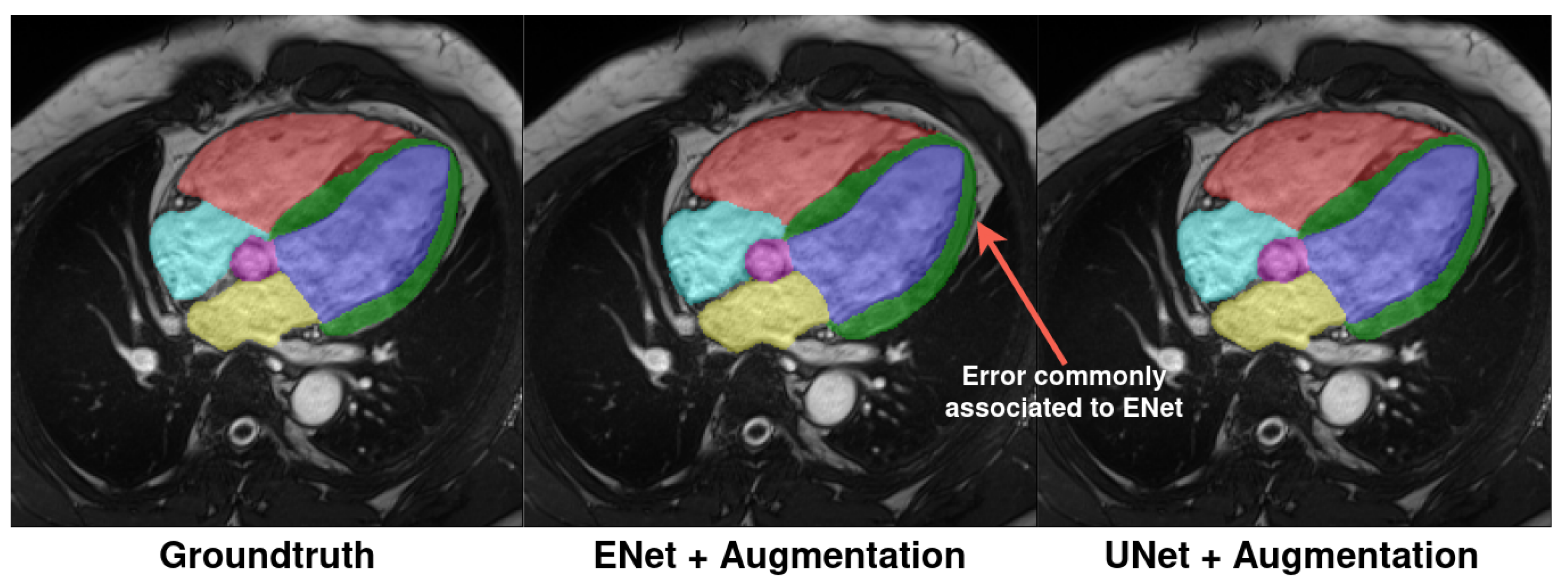
While a short comparison was performed with the state-of-the-art UNet architecture, further hyperparameter optimization, for instance over different loss functions, may provide deeper insights into the performance differences between the architectures.

6. Conclusions

In this work, we present an automated segmentation framework for the detection of anatomical structures on Cine-MRI LAX images, which exhibit more complex structures compared to the SAX orientation. We assess the effect of a comprehensive hierarchical data-augmentation strategy in detecting LAX anatomical structures, demonstrating its ability to produce robust results against anatomical anomalies and image degradation. The strategy has also shown its usefulness in producing acceptable segmentation outputs to compute the LVEF clinical metric, with Bland−Altman plots displaying a negligible bias over the four-chamber test set.

We demonstrate that the ENet CNN architecture is a viable option for whole-heart segmentation in both two- and four-chamber sequences, achieving acceptable results. The combination of an acceptable performance in both orientations along with the compact size of ENet makes this model attractive for practical real-time applications and deployment. While the segmentation may be less precise near anatomical frontiers with small overlaps, the obtained results make its use for clinical purposes feasible.

We also conducted a short comparison with a barebone UNet architecture, revealing slightly lower performances depending on the dataset. While it can be hypothesized that core conceptual differences come into play regarding the observed behaviors, this comparison would benefit from additional experiments to observe better characterization and highlight differences between the outputs produced by the two architectures.

References

1. Roth, G.A.; Mensah, G.A.; Johnson, C.O.; Addolorato, G.; Ammirati, E.; Baddour, L.M.; Barengo, N.C.; Beaton, A.Z.; Benjamin, E.J.; Benziger, C.P.; et al. Global Burden of Cardiovascular Diseases and Risk Factors, 1990–2019. J. Am. Coll. Cardiol. 2020, 76, 2982–3021. [Google Scholar] [CrossRef] [PubMed]
2. Vaduganathan, M.; Mensah, G.A.; Turco, J.V.; Fuster, V.; Roth, G.A. The Global Burden of Cardiovascular Diseases and Risk. J. Am. Coll. Cardiol. 2022, 80, 2361–2371. [Google Scholar] [CrossRef] [PubMed]
3. Karamitsos, T.D.; Francis, J.M.; Myerson, S.; Selvanayagam, J.B.; Neubauer, S. The Role of Cardiovascular Magnetic Resonance Imaging in Heart Failure. J. Am. Coll. Cardiol. 2009, 54, 1407–1424. [Google Scholar] [CrossRef] [PubMed]
4. Wang, L.; Wang, H.; Huang, Y.; Yan, B.; Chang, Z.; Liu, Z.; Zhao, M.; Cui, L.; Song, J.; Li, F. Trends in the application of deep learning networks in medical image analysis: Evolution between 2012 and 2020. Eur. J. Radiol. 2022, 146, 110069. [Google Scholar] [CrossRef] [PubMed]
5. Bernard, O.; Lalande, A.; Zotti, C.; Cervenansky, F.; Yang, X.; Heng, P.A.; Cetin, I.; Lekadir, K.; Camara, O.; Gonzalez Ballester, M.A.; et al. Deep Learning Techniques for Automatic MRI Cardiac Multi-Structures Segmentation and Diagnosis: Is the Problem Solved? IEEE Trans. Med. Imaging 2018, 37, 2514–2525. [Google Scholar] [CrossRef] [PubMed]
6. Fulton, M.J.; Heckman, C.R.; Rentschler, M.E. Deformable Bayesian convolutional networks for disease-robust cardiac MRI segmentation. In Proceedings of the International Workshop on Statistical Atlases and Computational Models of the Heart, Strasbourg, France, 27 September 2021; Springer: Berlin/Heidelberg, Germany, 2021; pp. 296–305. [Google Scholar]
7. Arega, T.W.; Legrand, F.; Bricq, S.; Meriaudeau, F. Using MRI-specific data augmentation to enhance the segmentation of right ventricle in multi-disease, multi-center and multi-view cardiac MRI. In Proceedings of the International Workshop on Statistical Atlases and Computational Models of the Heart, Strasbourg, France, 27 September 2021; Springer: Berlin/Heidelberg, Germany, 2021; pp. 250–258. [Google Scholar]
8. Punithakumar, K.; Carscadden, A.; Noga, M. Automated segmentation of the right ventricle from magnetic resonance imaging using deep convolutional neural networks. In Proceedings of the International Workshop on Statistical Atlases and Computational Models of the Heart, Strasbourg, France, 27 September 2021; Springer: Berlin/Heidelberg, Germany, 2021; pp. 344–351. [Google Scholar]
9. Li, L.; Ding, W.; Huang, L.; Zhuang, X. Right ventricular segmentation from short-and long-axis mris via information transition. In Proceedings of the International Workshop on Statistical Atlases and Computational Models of the Heart, Strasbourg, France, 27 September 2021; Springer: Berlin/Heidelberg, Germany, 2021; pp. 259–267. [Google Scholar]
10. Liu, D.; Yan, Z.; Chang, Q.; Axel, L.; Metaxas, D.N. Refined deep layer aggregation for multi-disease, multi-view & multi-center cardiac MR segmentation. In Proceedings of the International Workshop on Statistical Atlases and Computational Models of the Heart, Strasbourg, France, 27 September 2021; Springer: Berlin/Heidelberg, Germany, 2021; pp. 315–322. [Google Scholar]
11. Jabbar, S.; Bukhari, S.T.; Mohy-ud Din, H. Multi-view SA-LA Net: A framework for simultaneous segmentation of RV on multi-view cardiac MR Images. In Proceedings of the International Workshop on Statistical Atlases and Computational Models of the Heart, Strasbourg, France, 27 September 2021; Springer: Berlin/Heidelberg, Germany, 2021; pp. 277–286. [Google Scholar]
12. Queirós, S. Right ventricular segmentation in multi-view cardiac MRI using a unified U-net model. In Proceedings of the International Workshop on Statistical Atlases and Computational Models of the Heart, Strasbourg, France, 27 September 2021; Springer: Berlin/Heidelberg, Germany, 2021; pp. 287–295. [Google Scholar]
13. Vigneault, D.M.; Xie, W.; Ho, C.Y.; Bluemke, D.A.; Noble, J.A. Ω-Net (Omega-Net): Fully automatic, multi-view cardiac MR detection, orientation, and segmentation with deep neural networks. Med. Image Anal. 2018, 48, 95–106. [Google Scholar] [CrossRef] [PubMed]
14. Jaderberg, M.; Simonyan, K.; Zisserman, A.; Kavukcuoglu, k. Spatial Transformer Networks. In Proceedings of the Advances in Neural Information Processing Systems, Montreal, QC, Canada, 7–12 December 2015; Curran Associates, Inc.: Red Hook, NY, USA, 2015; Volume 28. [Google Scholar]
15. Bai, W.; Chen, C.; Tarroni, G.; Duan, J.; Guitton, F.; Petersen, S.E.; Guo, Y.; Matthews, P.M.; Rueckert, D. Self-Supervised Learning for Cardiac MR Image Segmentation by Anatomical Position Prediction. arXiv 2019, arXiv:1907.02757. [Google Scholar]
16. Bai, W.; Sinclair, M.; Tarroni, G.; Oktay, O.; Rajchl, M.; Vaillant, G.; Lee, A.; Aung, N.; Lukaschuk, E.; Sanghvi, M.; et al. Automated cardiovascular magnetic resonance image analysis with fully convolutional networks. J. Cardiovasc. Magn. Reson. 2018, 20, 65. [Google Scholar] [CrossRef]
17. Simonyan, K.; Zisserman, A. Very deep convolutional networks for large-scale image recognition. arXiv 2014, arXiv:1409.1556. [Google Scholar]
18. Acero, J.C.; Zacur, E.; Xu, H.; Ariga, R.; Bueno-Orovio, A.; Lamata, P.; Grau, V. SMOD - Data Augmentation Based on Statistical Models of Deformation to Enhance Segmentation in 2D Cine Cardiac MRI. In Functional Imaging and Modeling of the Heart; Springer: Berlin/Heidelberg, Germany, 2019; pp. 361–369. [Google Scholar] [CrossRef]
19. Al Khalil, Y.; Amirrajab, S.; Lorenz, C.; Weese, J.; Pluim, J.; Breeuwer, M. Reducing segmentation failures in cardiac MRI via late feature fusion and GAN-based augmentation. Comput. Biol. Med. 2023, 161, 106973. [Google Scholar] [CrossRef]
20. Al Khalil, Y.; Amirrajab, S.; Pluim, J.; Breeuwer, M. Late fusion U-Net with GAN-based augmentation for generalizable cardiac MRI segmentation. In Proceedings of the International Workshop on Statistical Atlases and Computational Models of the Heart, Strasbourg, France, 27 September 2021; Springer: Berlin/Heidelberg, Germany, 2021; pp. 360–373. [Google Scholar]
21. Pei, C.; Wu, F.; Huang, L.; Zhuang, X. Disentangle domain features for cross-modality cardiac image segmentation. Med. Image Anal. 2021, 71, 102078. [Google Scholar] [CrossRef] [PubMed]
22. Wang, R.; Zheng, G. CyCMIS: Cycle-consistent Cross-domain Medical Image Segmentation via diverse image augmentation. Med. Image Anal. 2022, 76, 102328. [Google Scholar] [CrossRef] [PubMed]
23. Martin-Isla, C.; Campello, V.; Izquierdo, C.; Kushibar, K.; Sendra-Balcells, C.; Gkontra, P.; Sojoudi, A.; Fulton, M.; Arega, T.; Punithakumar, K.; et al. Deep Learning Segmentation of the Right Ventricle in Cardiac MRI: The M&Ms Challenge. IEEE J. Biomed. Health Inform. 2023, 27, 3302–3313. [Google Scholar] [CrossRef] [PubMed]
24. Zhang, W.; Ding, X.; Liu, Y.; Qiao, B. Slide deep reinforcement learning networks: Application for left ventricle segmentation. Pattern Recognit. 2023, 141, 109667. [Google Scholar] [CrossRef]
25. Sinclair, M.; Bai, W.; Puyol-Antón, E.; Oktay, O.; Rueckert, D.; King, A.P. Fully automated segmentation-based respiratory motion correction of multiplanar cardiac magnetic resonance images for large-scale datasets. In Proceedings of the 20th International Conference of Medical Image Computing and Computer-Assisted Intervention (MICCAI 2017), Quebec City, QC, Canada, 11–13 September 2017; Proceedings, Part II 20. Springer: Berlin/Heidelberg, Germany, 2017; pp. 332–340. [Google Scholar]
26. Leng, S.; Yang, X.; Zhao, X.; Zeng, Z.; Su, Y.; Koh, A.S.; Sim, D.; Le Tan, J.; San Tan, R.; Zhong, L. Computational platform based on deep learning for segmenting ventricular endocardium in long-axis cardiac MR imaging. In Proceedings of the 2018 40th Annual International Conference of the IEEE Engineering in Medicine and Biology Society (EMBC), Honolulu, HI, USA, 18–21 July 2018; pp. 4500–4503. [Google Scholar]
27. Zhang, X.; Noga, M.; Martin, D.G.; Punithakumar, K. Fully automated left atrium segmentation from anatomical cine long-axis MRI sequences using deep convolutional neural network with unscented Kalman filter. Med. Image Anal. 2021, 68, 101916. [Google Scholar] [CrossRef] [PubMed]
28. Gonzales, R.; Seemann, F.; Lamy, J.; Arvidsson, P.; Heiberg, E.; Murray, V.; Peters, D. Automated left atrial time-resolved segmentation in MRI long-axis cine images using active contours. BMC Med. Imaging 2021, 21, 101. [Google Scholar] [CrossRef] [PubMed]
29. Ronneberger, O.; Fischer, P.; Brox, T. U-Net: Convolutional Networks for Biomedical Image Segmentation. In Proceedings of the Medical Image Computing and Computer-Assisted Intervention (MICCAI 2015), Munich, Germany, 5–9 October 2015; Navab, N., Hornegger, J., Wells, W.M., Frangi, A.F., Eds.; Springer: Cham, Switzerland, 2015; pp. 234–241. [Google Scholar]
30. Azad, R.; Aghdam, E.K.; Rauland, A.; Jia, Y.; Avval, A.H.; Bozorgpour, A.; Karimijafarbigloo, S.; Cohen, J.P.; Adeli, E.; Merhof, D. Medical image segmentation review: The success of u-net. arXiv 2022, arXiv:2211.14830. [Google Scholar]
31. Yin, X.X.; Sun, L.; Fu, Y.; Lu, R.; Zhang, Y. U-Net-Based medical image segmentation. J. Healthc. Eng. 2022, 2022, 4189781. [Google Scholar] [CrossRef]
32. Huang, H.; Lin, L.; Tong, R.; Hu, H.; Zhang, Q.; Iwamoto, Y.; Han, X.; Chen, Y.; Wu, J. UNet 3+: A Full-Scale Connected UNet for Medical Image Segmentation. In Proceedings of the ICASSP 2020—2020 IEEE International Conference on Acoustics, Speech and Signal Processing (ICASSP), Barcelona, Spain, 4–8 May 2020; pp. 1055–1059. [Google Scholar]
33. Paszke, A.; Chaurasia, A.; Kim, S.; Culurciello, E. Enet: A deep neural network architecture for real-time semantic segmentation. arXiv 2016, arXiv:1606.02147. [Google Scholar]
34. Salvaggio, G.; Comelli, A.; Portoghese, M.; Cutaia, G.; Cannella, R.; Vernuccio, F.; Stefano, A.; Dispensa, N.; Tona, G.L.; Salvaggio, L.; et al. Deep Learning Network for Segmentation of the Prostate Gland with Median Lobe Enlargement in T2-weighted MR Images: Comparison with Manual Segmentation Method. Curr. Probl. Diagn. Radiol. 2021, 51, 328–333. [Google Scholar] [CrossRef]
35. Lieman-Sifry, J.; Le, M.; Lau, F.; Sall, S.; Golden, D. FastVentricle: Cardiac segmentation with ENet. In Proceedings of the International Conference on Functional Imaging and Modeling of the Heart, Toronto, ON, Canada, 11–13 June 2017; Springer: Berlin/Heidelberg, Germany, 2017; pp. 127–138. [Google Scholar]
36. Painchaud, N.; Skandarani, Y.; Judge, T.; Bernard, O.; Lalande, A.; Jodoin, P.M. Cardiac segmentation with strong anatomical guarantees. IEEE Trans. Med. Imaging 2020, 39, 3703–3713. [Google Scholar] [CrossRef] [PubMed]
37. Karimov, A.; Razumov, A.; Manbatchurina, R.; Simonova, K.; Donets, I.; Vlasova, A.; Khramtsova, Y.S.; Ushenin, K. Comparison of UNet, ENet, and BoxENet for Segmentation of Mast Cells in Scans of Histological Slices. In Proceedings of the 2019 International Multi-Conference on Engineering, Computer and Information Sciences (SIBIRCON), Novosibirsk, Russia, 21–27 October 2019; pp. 544–547. [Google Scholar]
38. Kadish, A.H.; Bello, D.; Finn, J.P.; Bonow, R.O.; Schaechter, A.; Subacius, H.P.; Albert, C.M.; Daubert, J.P.; Fonseca, C.G.; Goldberger, J.J. Rationale and Design for the Defibrillators to Reduce Risk by Magnetic Resonance Imaging Evaluation (DETERMINE) Trial. J. Cardiovasc. Electrophysiol. 2009, 20, 982–987. [Google Scholar] [CrossRef] [PubMed]
39. Suinesiaputra, A.; Cowan, B.R.; Al-Agamy, A.O.; Elattar, M.A.; Ayache, N.; Fahmy, A.S.; Khalifa, A.M.; Medrano-Gracia, P.; Jolly, M.-P.; Kadish, A.H.D.; et al. A collaborative resource to build consensus for automated left ventricular segmentation of cardiac MR images. Med. Image Anal. 2014, 18, 50–62. [Google Scholar] [CrossRef] [PubMed]
40. Kingma, D.P.; Ba, J. Adam: A method for stochastic optimization. arXiv 2014, arXiv:1412.6980. [Google Scholar]
41. Zotti, C.; Luo, Z.; Lalande, A.; Jodoin, P.M. Convolutional neural network with shape prior applied to cardiac MRI segmentation. IEEE J. Biomed. Health Inform. 2018, 23, 1119–1128. [Google Scholar] [CrossRef]
42. Bulwer, B.E.; Solomon, S.D.; Janardhanan, R. Echocardiographic assessment of ventricular systolic function. In Essential Echocardiography: A Practical Handbook with DVD; Springer: Berlin/Heidelberg, Germany, 2007; pp. 89–117. [Google Scholar]
43. Beetz, M.; Corral Acero, J.; Grau, V. A Multi-View Crossover Attention U-Net Cascade with Fourier Domain Adaptation for Multi-Domain Cardiac MRI Segmentation. In Proceedings of the Statistical Atlases and Computational Models of the Heart. Multi-Disease, Multi-View, and Multi-Center Right Ventricular Segmentation in Cardiac MRI Challenge: 12th International Workshop (STACOM 2021), Held in Conjunction with (MICCAI 2021), Strasbourg, France, 27 September 2021; pp. 323–334. [Google Scholar] [CrossRef]
Figure 1. An example of a visible anomaly (right) compared to normal case (left) in LAX 2-chamber view, at the level of the apex (and not visible in SAX). The anomaly is the result of a localized aneurysm in the apical region. The condition is concomitant to hypertrophic cardiomyopathy and exhibits a thickened myocardium wall. The presented images are part of a Cine-MRI sequence.
Algorithms 17 00010 g001
Figure 2. The ENet architecture (bottom) depicting the initial block (top left), the bottleneck module (top right) and the complete architecture (bottom). The output shapes are shown for an input image of size 256 × 256 with and an output of C classes. conv is either a regular, dilated or full convolution (also known as 3 × 3 filters or a 5 × 5 convolution decomposed into two asymmetric ones).
Algorithms 17 00010 g002
Figure 3. Hierarchical procedure followed for data augmentation. Amount of rotations and flipping presence were varied across the different configurations.
Algorithms 17 00010 g003
Figure 4. Results obtained with ENet on test sets. Darker plots correspond to data-augmented scores. Mean values are represented as red crosses. Hausdorff distances are represented on a logarithmic scale for better readability.
Algorithms 17 00010 g004
Figure 5. Bland−Altman plots obtained over 2- and 4-chamber test sets with augmented and nonaugmented models. A positive bias is observed with 2-chamber models in agreement with results reported in Table 2.
Algorithms 17 00010 g005
Figure 6. Cross-validation scores for each of the trained folds. Cross-validation results using a UNet architecture are also shown here to provide further evidence of consistency of the models and datasets.
Algorithms 17 00010 g006
Figure 7. Average metric curves over different data-augmentation configurations. Nonaugmented and best average configuration performance-wise (presented in Table 1, Table 4 and Table 6) are emphasized in bold.
Algorithms 17 00010 g007
Figure 8. Comparison of Dice score improvement between 2- and 4-chamber views with different amounts of data. Experiments were conducted with shared dataset sizes of 250 and 500 examinations in addition to originally available data.
Algorithms 17 00010 g008
Figure 9. Examples of various difficult scenarios encountered in 2-chamber (a) and 4-chamber (b,c) views. In (a), the following color scheme is used: LA = red, LVC = blue and MYO = green. In (b,c) the following color scheme is used: RV = red, LVC = blue, MYO = green, LA = yellow, RA = cyan and AO = purple. It is also worth noting that the aortic root was detected in row (b) thanks to data augmentation. * Examination extracted from validation set.
Algorithms 17 00010 g009
Figure 10. Example of typical errors produced by ENet architecture compared to ground truth and UNet prediction. A small overlap outside of the real myocardium is visible. The same color scheme from Figure 9 is applied.
Algorithms 17 00010 g010