Article

Frequent Errors in Modeling by Machine Learning: A Prototype Case of Predicting the Timely Evolution of COVID-19 Pandemic
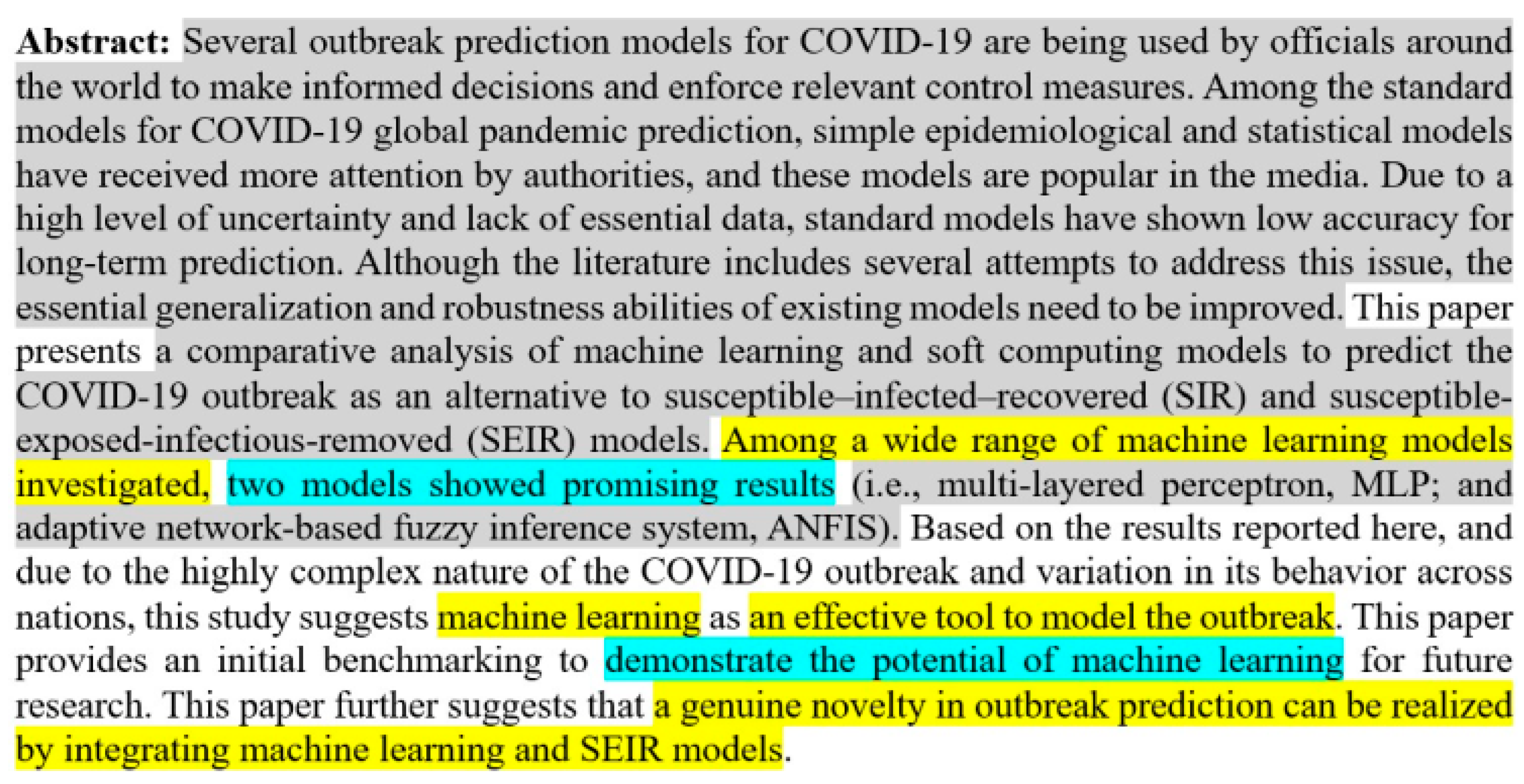
by
Károly Héberger
Plasma Chemistry Research Group, Institute of Materials and Environmental Chemistry, HUN-REN Research Centre for Natural Sciences, Institute of Excellence, Hungarian Academy of Sciences, Magyar tudósok krt. 2., H-1117 Budapest, Hungary
Algorithms 2024, 17(1), 43; https://doi.org/10.3390/a17010043
Submission received: 22 December 2023 / Accepted: 8 January 2024 / Published: 19 January 2024
(This article belongs to the Special Issue Supervised and Unsupervised Classification Algorithms (2nd Edition))

Abstract

:
Background: The development and application of machine learning (ML) methods have become so fast that almost nobody can follow their developments in every detail. It is no wonder that numerous errors and inconsistencies in their usage have also spread with a similar speed independently from the tasks: regression and classification. This work summarizes frequent errors committed by certain authors with the aim of helping scientists to avoid them. Methods: The principle of parsimony governs the train of thought. Fair method comparison can be completed with multicriteria decision-making techniques, preferably by the sum of ranking differences (SRD). Its coupling with analysis of variance (ANOVA) decomposes the effects of several factors. Earlier findings are summarized in a review-like manner: the abuse of the correlation coefficient and proper practices for model discrimination are also outlined. Results: Using an illustrative example, the correct practice and the methodology are summarized as guidelines for model discrimination, and for minimizing the prediction errors. The following factors are all prerequisites for successful modeling: proper data preprocessing, statistical tests, suitable performance parameters, appropriate degrees of freedom, fair comparison of models, and outlier detection, just to name a few. A checklist is provided in a tutorial manner on how to present ML modeling properly. The advocated practices are reviewed shortly in the discussion. Conclusions: Many of the errors can easily be filtered out with careful reviewing. Every authors’ responsibility is to adhere to the rules of modeling and validation. A representative sampling of recent literature outlines correct practices and emphasizes that no error-free publication exists.

Graphical Abstract

1. Introduction

János Máttyus Nepomuk published a book entitled Horse Science in 1845 [1]. One of its figures includes a sick horse, on which all the external and internal horse diseases are indicated that can affect the animal during its life (Figure 1). Naturally, such an animal cannot exist; still, it is used figuratively in the Hungarian language (“állatorvosi ló”, i.e., “veterinary horse”). One cannot find a scientific article that commits all possible (known) errors, but a recent, highly cited paper [2] can be used as a prototype for illustrative purposes. In this paper, I will summarize the correct practice and the methodology to be followed for model discrimination.
The existence of any “scientific method” is seriously questioned by the appearance of Kuhn’s book, The Structure of Scientific Revolutions [3]. However, there are many rules, and standards which govern scientific investigation, e.g., the principle of parsimony (Occam’s razor) [4] declares: “Entities should not be multiplied beyond necessity”. Consequently, if we have different explanations of the observed data, the simplest one should be preferred. In other words: if two models provide the same description (prediction) in the statistical sense, the simpler one should be accepted. Occam’s razor is a sort of universal feature pervading nearly all fields of science. Machine learning, deep learning, etc. might violate the principle of parsimony on a large scale, while they usually provide state-of-the-art predictive performance on large datasets. Over- and underdetermined models are routinely used for prediction. Breiman called attention to the two cultures in statistics (and generally in data science) [5]: one is based on a stochastic data model, whereas the other is based on algorithmic models and assumes that the data mechanism is unknown. Ardabilli et al.’s paper [2] belongs to the latter culture definitely. Hence, rigid adherence to Occam’s razor cannot be expected. However, algorithmic modeling should only be used on large, complex datasets, but not for “small” datasets.
Let us return to Earth from the philosophical heights. Consistent notation is a prerequisite in scientific communication, as described in detail in ref. [6].
The proper method comparison has been pioneered by Frank and Friedman [7] using simulated datasets (five algorithms, 36 situations, the performance was measured by the distance to the true model and by the average squared prediction error).
A recent review (personal reminiscences) [8] summarizes the modeling procedure according to the OECD principles and regulations, with a detailed discussion on the steps of modeling procedure, genetic algorithm, rigorous validation, external test sets, performance parameters, variable selection, avoiding chance correlations, giving the applicability domain, consensus modeling and alike. Quantitative Structure–Activity Relationship modeling is analogous to ML modeling completely in this sense.
After the above short summary on how to perform statistical modeling, it is high time to define the aims of the present work: (i) collecting the frequent errors committed by certain authors with the intention of helping scientists to avoid them and by no means humiliate people, who are not aware of the present status of knowledge. (ii) Specifically, the following goals can be formulated for forecasting the epidemic: Can the progress of the COVID-19 epidemic be modeled with machine learning (ML) algorithms? Can useful predictions be made? Which algorithm is the best? Of course, the answer is yes to all questions, it is possible, and it can be. The best model can be selected, and even the models can be ranked in a rigorous manner. The question remains how, and how to do it properly in a scientifically sound manner.
The gathered errors and recommendations have far-reaching consequences: The publisher MDPI should revise its editorial policy, and rejection should be default if the results/discussion and conclusions contradict each other or a certain level (number) of errors found. The above and similar crucial errors indicate that the reviewers have NOT read the manuscripts entirely. Sloppy reviewers should be banned from further reviewing at least for a certain period (e.g., for five or ten years). Reviewers and authors alike should go through the checklist (Section 3.11) to help optimal progress in science.
New, multicriteria optimization (SRD) calculations and ANOVA have been made (Section 3.3,Section 3.6 and Section 3.7) to reveal outliers and to illustrate that even a wrong starting point may lead to an appropriate conclusion. Moreover, this work aims to gather the correct practices of model discrimination, usage of performance parameters, fair model comparison, and alike.

2. Materials and Methods
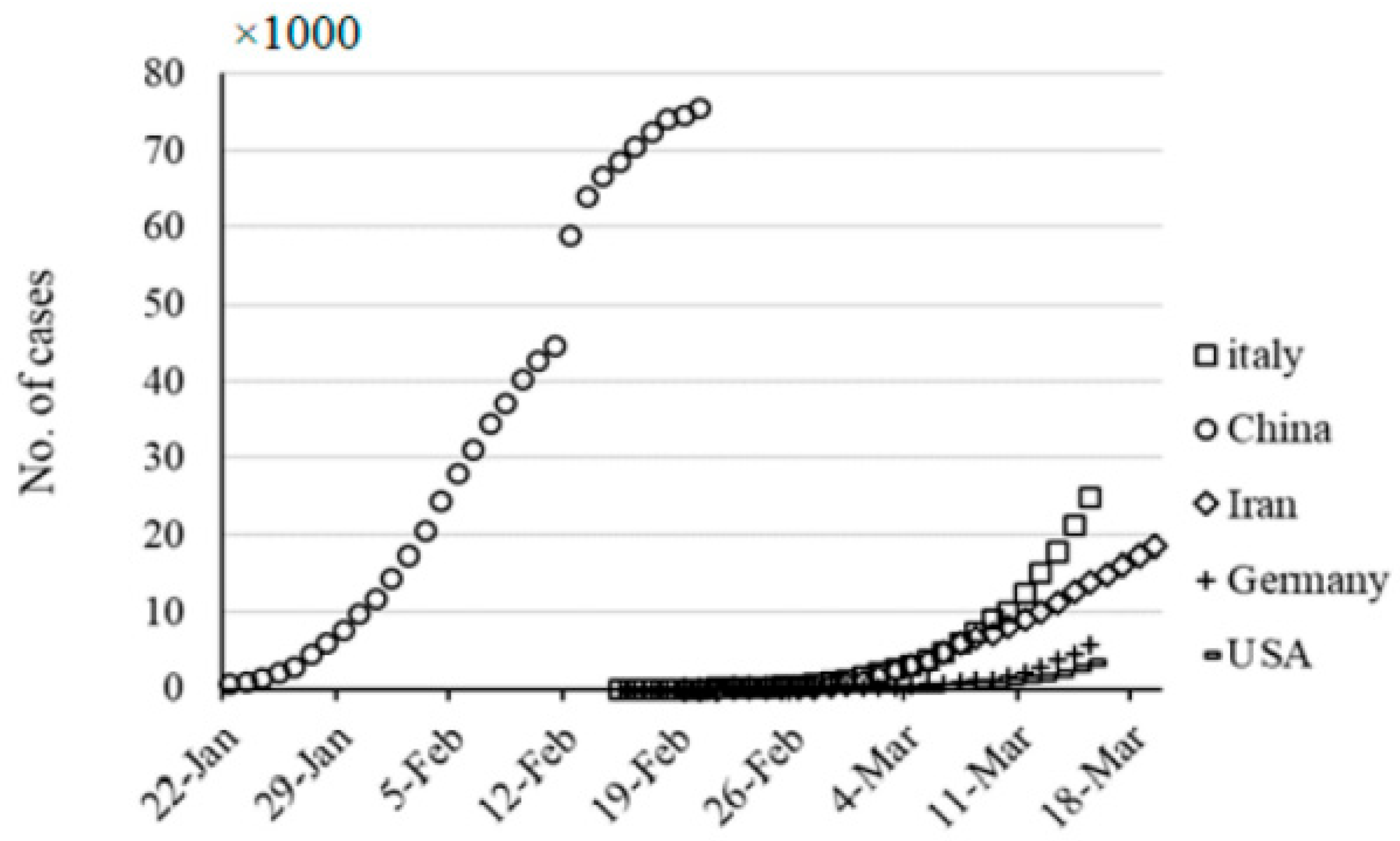
2.1. Data

The cumulative number of cases [number of infected persons] for five countries over 30 days served as the basis of investigation (Figure 2). The starting date and evolution are different. There is no reason given why the time interval is limited when wider ranges are readily available. The outcome of the investigations does not justify urgency; several months of waiting would be warranted.

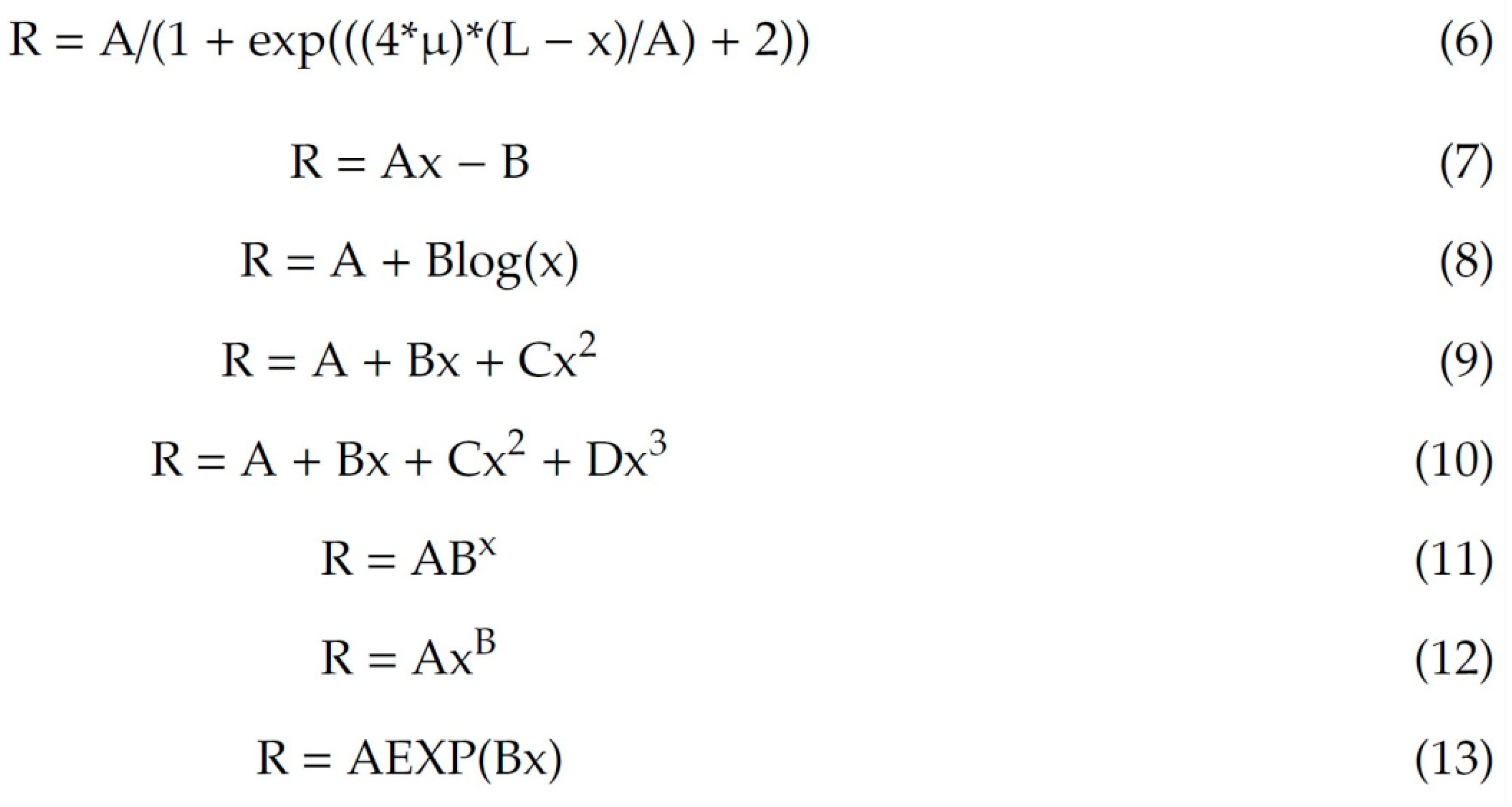
2.2. Models to Be Compared

Eight models have been compared; see Figure 3, including logistic (Lgs), linear (Lin), logarithmic (Lgt), quadratic (Qad), cubic (Cub), compound (Cop), power (Pow), and exponential (Exp) equations, respectively, where A, B, C, µ, and L are parameters (constants) to be fitted.
It should be noted that the exponential equation has been proven inappropriate in a previous part of ref. [2]: Equation (4) of ref. [2] has been derived from differential equations and contains a misprint; the time (t) is missing from the right-hand side.

2.3. Algorithms for Searching Global Minimum

Perhaps the first one was the simulated annealing [9] followed by tabu search [10] dating back to the 1980s. A series of nature-inspired algorithms were elaborated after that, including genetic algorithm (GA) [11] and particle swarm optimization (PSO) [12]. Year to year, a novel framework was found for nature-inspired optimizations: e.g., Ant Colony Optimization (ACO) [13]. Honey Bee Optimization (HBO) was inspired by the foraging behavior of honey bees, and thus it uses employed bees, onlooker bees, and scout bees to explore the search space [14]. It was immediately developed into the Artificial Bee Colony Algorithm (ABC) [15]. Firefly Algorithm (FA) copied the flashing behavior of fireflies [16]; Cuckoo Search (CS) involves a population of nests (solutions) where cuckoos lay their eggs (candidate solutions) [17]. Krill Herd Optimization [18] was followed by grey wolf optimizer (GWO), which mimics the hunting behavior of grey wolves and involves three types of wolves (alpha, beta, and delta) that simulate the leadership hierarchy in a wolf pack [19], not to speak about many more. All the above are search algorithms aimed at finding the proximity of the global minimum. All have some “tricks” to escape local minima. They do not give one single best solution, but a population of candidate (good) solutions. They tend to be hybridized, i.e., coupled with other techniques to find the exact global minimum. All have some kind of hierarchical organization and regularization (meta) parameters, and their initial choice greatly determines their performance. It is worth running the computer codes multiple times with random initialization.

2.4. Fair Method (Model) Comparison

A proven algorithm for fair model comparison is called the sum of ranking differences (SRDs) as described in ref. [20]; its extension to input matrices containing equal numbers (ties) has been published in 2013 [21]. A link to a downloadable program can be found here [22]. Two validation options are available: randomization test [23] and cross-validation [23] with the application of the Wilcoxon test [24]. Although SRD was primarily developed to solve model comparison problems, it realizes multicriteria optimization [25], as long as the input matrix is arranged as such: alternatives in the columns and features (criteria) in the rows.

3. Results and Discussion

3.1. Contradictions in Abstract, Discussion and Conclusion

Let us start with the abstract of ref. [2] (Figure 4).
The guidelines of MDPI journals suggest the partitioning of the abstract into four parts (background, methods, results, and conclusions). Figure 4 shows unbalanced partitioning, to say the least. There are few or no results written in the middle gray part (starting at sentence five): SIR and SEIR do not embody the results of the authors’ work, and only two machine learning algorithms, MLP and ANFIS, were examined there. It is simply impossible to generalize these findings to the “wide range of machine learning models”. The models provided in Figure 3 are not ML, but causal ones or their approximations. Algorithms for finding the global minimum (Section 2.3) are not machine learning algorithms, either. It should be noted that physicists tend to confuse ML and deep learning, although ML is not a method of artificial intelligence (AI).
The authors are probably not aware of the English understatement. Science is international and binds different cultures together. It is not appropriate to hurt anybody, and cautious formulation is mandatory. As a consequence, “promising results” and great “potential” mean just the opposite, c.f., ref. [26]. The advocated policy is to express the results explicitly, preferably with numbers and without quality terms, e.g., “successful” modeling means nothing. The reader should decide whether the modeling is successful or rudimentary. Dubious formulations should be avoided.
It is difficult to decide the truthfulness of the statements marked by yellow. I am deeply convinced that properly applied machine learning algorithms can effectively model the outbreak of the epidemic. However, the results of these investigations [2] indicate the opposite as was stated in the discussion section: “Extrapolation of the prediction beyond the original observation range of 30 days should not be expected to be realistic considering the new statistics” [2] and “The fitted models generally showed low accuracy and also weak generalization ability for the five countries” [2].
Another point is whether to publish negative results. Many scientists advocate against it, while others find them useful for the scientific community: we can avoid reproducing experiments with hopeless outcomes, thereby saving money and energy for new experiments and calculations. Therefore, it is a matter of opinion whether to report negative results. I am inclined to say yes, but in the context of a failure only; in that case, the conclusions should have been read as the following: “… advancement of global models with generalization ability would not be feasible” and “… it is not possible to select the most suitable scenario” [2]. The authors honestly admit the fallacious modeling in the discussion section, but then they conclude that “machine learning [is] an effective tool to model the outbreak”. Why? Why did the editor and the reviewers not notice this? Even less understandable is the next statement that occurs twice in the paper: “a genuine novelty in outbreak prediction can be realized by integrating machine learning and SEIR models”, especially if we see that no such integration was involved in the study.
The only plausible explanation for such contradictions can be that neither the editor nor the reviewers read the manuscript fully, if the authors. The authorship is to be determined by the Vancouver criteria [27] (see Appendix A) as prescribed by the ethical guide of MDPI (https://www.mdpi.com/ethics#_bookmark2 (accessed on 9 January 2024)).

3.2. Model Comparison

Ref. [2] clearly defines the aim: “This paper aims to investigate the generalization ability of the proposed ML models and the accuracy of the proposed models for different lead times”. Figure 3 collects the models to be compared: all models (with one exception) are linear or linear in parameters (curvilinear), or easily linearizable by logarithmic transformation. That is, the normal equations can be solved easily in closed form. For example, the estimated parameters of Equation (7) in Figure 3 by maximum likelihood ( A ^ and B ^ ) can be calculated without any minimum search (using the notations of Equation (7) in Figure 3):
A ^ = n i n x i R i i n x i i n R i n i n x i 2 i n x i 2
And
B ^ = b x ¯ R ¯
What is the need to apply search algorithms when solutions are readily available? Why is it necessary to fit the models by global optimization algorithms (which are developed for complicated problems, implicit dependent variables, and many hundreds or even thousands of parameters and variables)? Similarly, all parameters of other models (except the logistic one) can be derived easily by solving the normal equations (eventually after logarithmic transformation). Logistic regression can also be solved by iteration easily without the usage of global optimization algorithms. In other words, the principle of parsimony was neglected or overlooked without any justification.

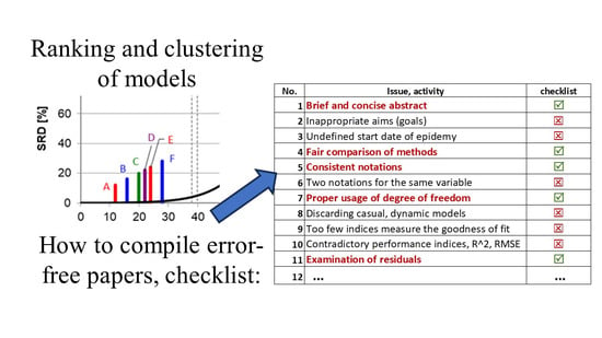
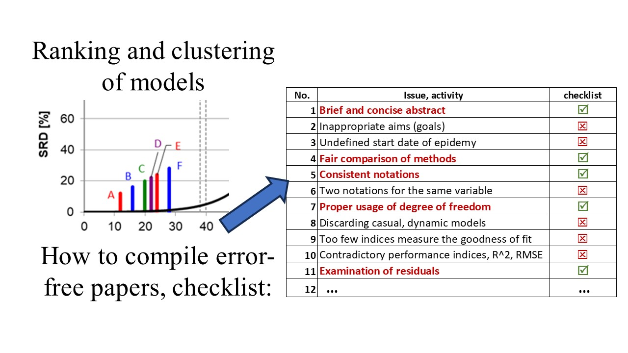
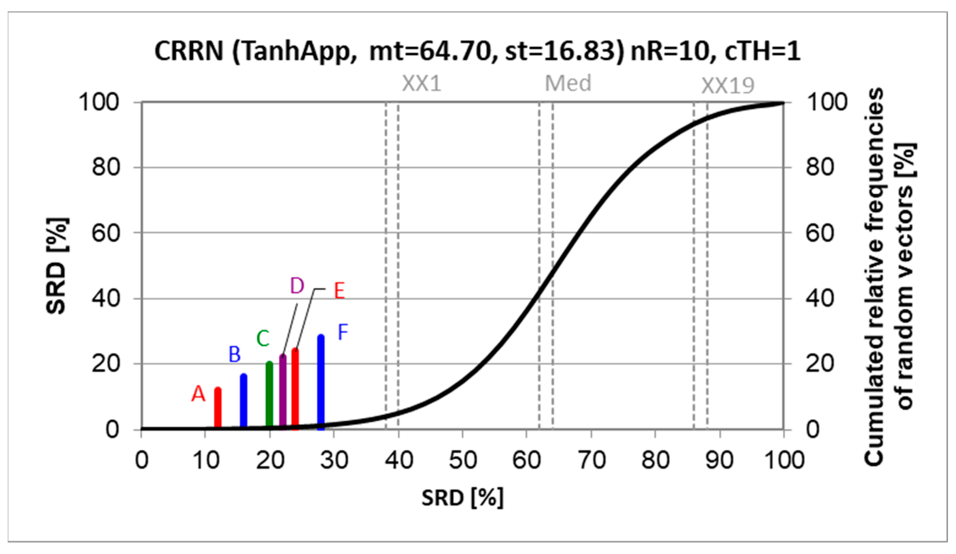
3.3. Model Comparison by Sum of Ranking Differences

Let us be good natured (benevolent) and assume that estimating the course of the epidemic in five countries starting at different times is a reasonable goal. (I personally disagree, but we can assume it). Eight models (summarized in Figure 3) were compared by using three minimum search algorithms (GA, PSO, and GWO), for 24 combinations altogether. Why just these algorithms were selected from the plethora of available ones (c.f., Section 2.3) is unknown. Fortunately, the authors provided detailed tables (Tables 3–10 in ref. [2]) with two evaluation (performance) criteria: correlation coefficient (r) and root mean square error (RMSE).
A data table can be constructed from r and RMSE in the rows and algorithm combinations to be compared in the columns. Row maxima for r and row minima for RMSE served as the benchmark reference. Such a benchmark realizes the hypothetical best combination: the largest correlation coefficients and the smallest residual errors. The proximity of the different alternatives to the hypothetical best combination is measured by SRD.
Figure 5 shows the SRD values and the cumulated relative frequencies of random ranking.
Even a superficial evaluation reveals that something is not in order. No clear winner can be established, neither from the models nor from the minimum search algorithms, though some tendencies are observed. Why could not all minimum search algorithms find the global minimum? They should! The possible reasons might be stopping too early, wrong starting values, running into local minima, the presence of outliers, or a combination of these reasons.

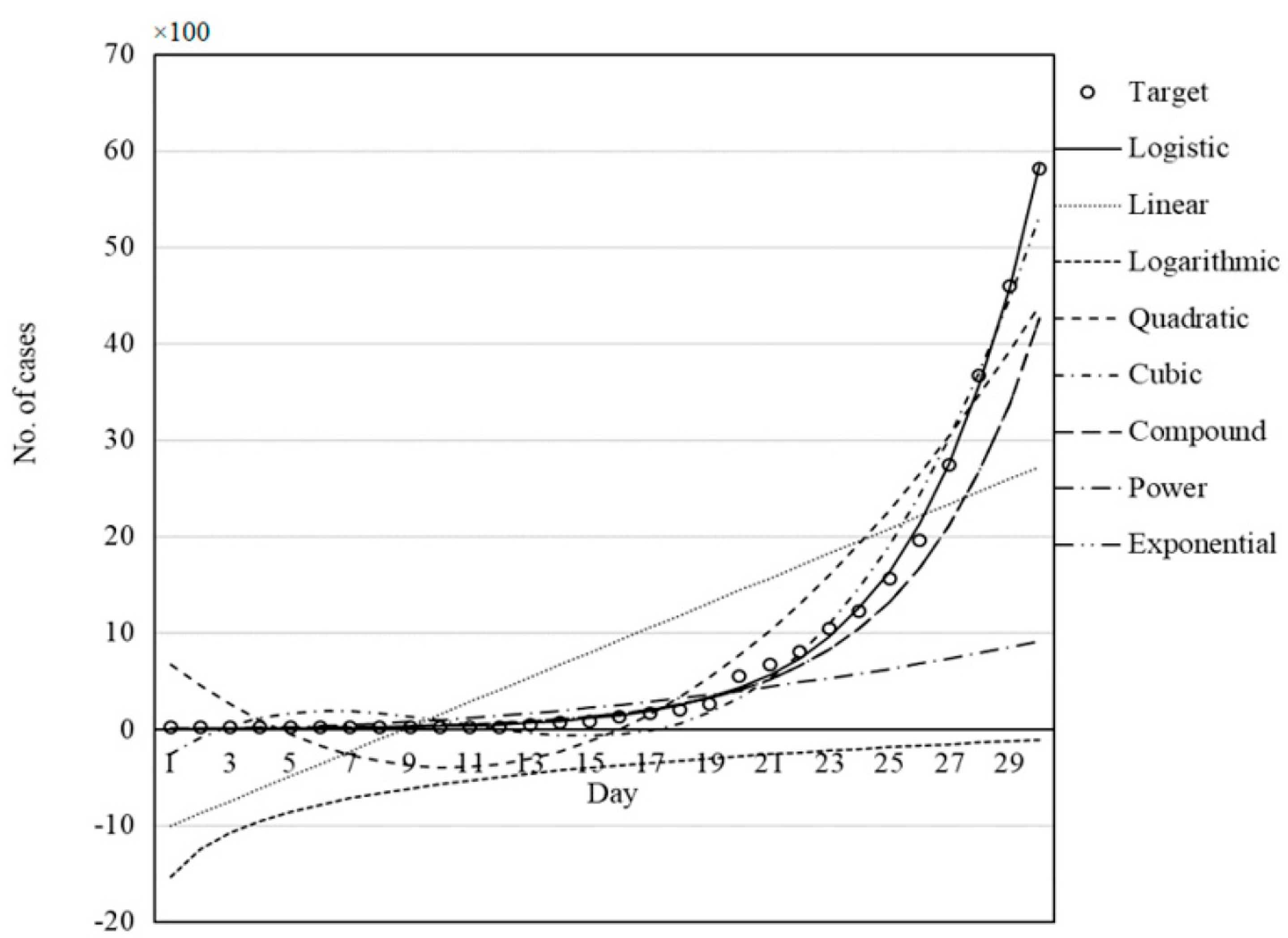
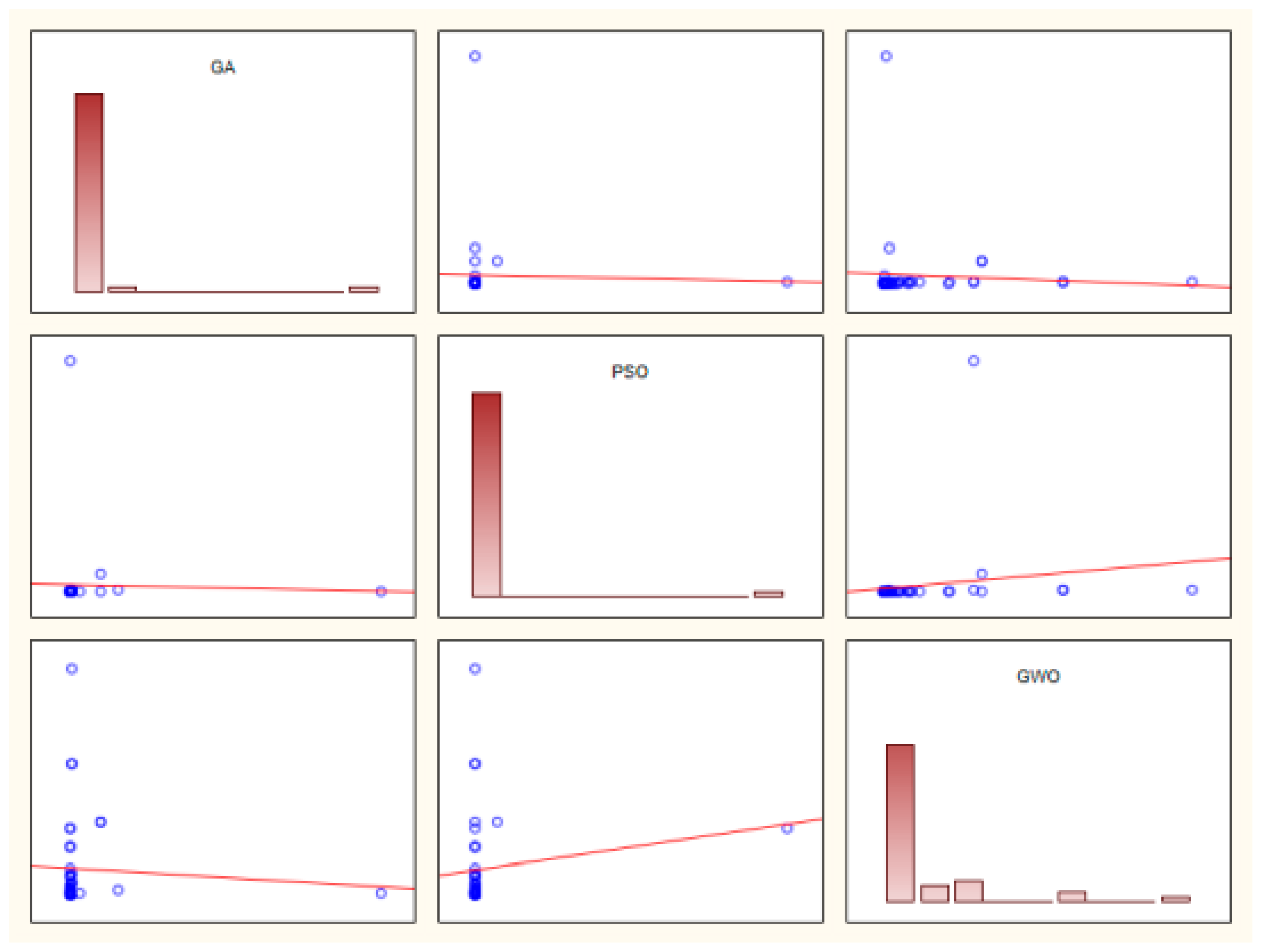
3.4. Visual Inspection

Let us see Figure 6 (Figure 10 of ref. [2]), where the performance of all models (in Figure 3) was compared for the description of the epidemic data of Germany by GWO.
Although a residual picture would be better, even a layman can judge that all models are inadequate except the logistic one. Why are they aiming to test them? Some of the models are completely worthless (linear, quadratic, cubic, and logarithmic ones), where negative numbers of infected persons are predicted. The authors should have paid attention to the positivity constraint. Similarly disappointing is the description of a monotone increasing (concave) curve with a convex one or one that exhibits a minimum. The same statements are valid for all the countries examined. The exponential and logistic functions run together; they are indistinguishable from each other in a visual evaluation. Both models have similar theoretical backgrounds; they can be derived from differential equations. Which one is better and/or adequate? The adequacy can be determined by visual assessment, too. If both models seem to be adequate, then a decision can be made by penalization of models using more fitting parameters: the logistic function uses four, while the exponential has two parameters only. Whether their difference is significant can, and should, be tested by setting null and alternative hypotheses, H0 and Ha, respectively. How to do it—will be discussed in the next section.

3.5. Performance Parameters (Merits) and Model Discrimination

Two performance parameters (r and RMSE) are not sufficient. Eight to twelve parameters are commonly used in the recent literature [28,29,30]. The usage of performance parameters differently for training and test sets has not been mentioned, either. Training and testing were used in the context of artificial neural networks (ANN), which are superfluous there, as parameter estimation can be completed without them. The description of MLP and ANFIS is no less than breaking a butterfly in a wheel. Similarly, over- and underfitting have not even been mentioned, along with bias-variance trade-off, although online course(s) are also available [31]. It should be mentioned that many performance parameters would provide a more sophisticated evaluation, and they are recommended below:
Mean absolute error (MAE) is a straightforward metric because it is simple and easily interpretable to estimate the accuracy of predictive models.
The Bayesian Information Criterion (BIC) is applied for model selection from among several rival models. It takes into account the degrees of freedom and penalizes more complex models with the number of parameters to avoid overfitting [32].
Akaike’s Information Criterion (AIC) is also a measure of the goodness of fit. AIC (similarly to BIC) is widely used for model selection from among numerous models [33]. BIC penalizes complex models more heavily than AIC does.
Instead of the number of point pairs (N) used in the denominator of the RMSE formula in ref. [2], the degrees of freedom would have been the proper choice: (Np), where p is the number of parameters in the models. As the number of parameters in all models is known (c.f., Figure 3), one can only wonder why the degrees of freedom were not considered, at all.
There are some unorthodox behaviors of the simple correlation coefficient as defined between independent (input) variables and dependent (output) variables. It can measure linear relations only, but some of the models—Equations (11)–(13) in ref. [2]—are highly nonlinear. On the other hand, a simple quadratic relation (parabola y = x2) would provide exactly r = 0 (if all plus minus pairs are involved). Naturally, a multiple correlation coefficient (index) can be defined, although differently, between the input y and output y ^ variables ( y ¯ is the mean of all y i -s):
R 1 2 = i N y ^ i y ¯ 2 i N y i y ¯ 2
Equation (3) was suggested by Draper and Smith [34] and it can have values larger than 1 for nonlinear equations (but not necessarily).
R 2 2 = 1 i N y i y ^ i 2 i N y i y ¯ 2
Equation (4) is often called determination coefficient in analytical chemistry textbooks. I found the first occurrence in ref. [35]. It cannot be larger than 1, but it can have negative values, if the model is worse than a simple constant, the average of all y i -s.
R 3 2 = i N y ^ i y ¯ 2 2 i N y i y ¯ 2 i N y ^ i y ^ ¯ 2
Equation (5) [36] also might suffer from being greater than 1 in the case of nonlinear models.
R 4 2 = i N y i y ¯ i N y ^ i y ^ ¯ 2 i N y i y ¯ 2 i N y ^ i y ^ ¯ 2
Equation (6) eliminates the inconsistent behavior detailed above for ( R 1 2 , R 2 2 , R 3 2 ). To my knowledge, Prof. Rolf Manne (University of Bergen) derived Equation (6) but never published it, and his equation is not used widely, if at all.
None of the above four equations has been applied in ref. [2] for model discrimination. The comparison of correlation indices, their features, and idiosyncrasies were first summarized in ref. [37]. It should be noted that adjusted (multiple) correlation coefficients should be used for model discrimination when the degrees of freedom are available (present case).
What remains is the residual error. Its examination reveals whether the modeling is adequate or not. It is suitable for comparing linear and nonlinear methods; even statistical testing is possible (F test can be applied as a variance ratio test). Three variants of F-tests might be feasible (practicable) [38].
(i) Ratio of residual variances (sum of squares, if the degree of freedom is equal, or known):
F c = s 1 2 s 2 2
where s 1 2 , s 2 2 are the residual variances for model 1 and model 2 to be compared, respectively. The residual variance is to be calculated using the degree of freedom (υ = N p ), where p is the number of parameters (two to four, c.f., Figure 3):
s 2 = R S S υ = i N y i y ^ i 2 N p
F c should be compared to the tabulated F value: F t a b υ 1 , υ 2 , 0.95   , if the F c is larger than the tabulated F value, then the null hypotheses should be rejected (H0, i.e., no significant differences are in the variances of the models). The power of F c is “small”, i.e., only large differences are detected (also called conservative estimation) so, a better option might be the following:
(ii) Partial F test:
F p = R S S e x t e n d e d R S S s i m p l e r s 2 s i m p l e r
where RSS is the residual sum of squares (nominator of Equation (8)). Strictly speaking, the partial F test has been developed to add in and remove variables from a linear model. Formally, linear, and nonlinear models can also be compared (if the numbers of parameters are the same) as if “curvature” was introduced in the model. F p should be compared to the tabulated F value: F t a b 1 , υ 2 , 0.95   , where υ 2 is the degree of freedom of the simpler model.
(iii) The termination criteria were suggested for models having nonlinearity [39]. Two models termed 2 and 1 can be compared using the sequential probability ratio:
S P R = s 2 s 1 N
The SPR value must be compared with the numbers A and B from critical tables. If SPRA, then model 1 is to be accepted. If SPRB, then model 2 is to be accepted. If B < SPR < A, then no decision can be made (more information is needed, i.e., more data and more measurements). For a double 95% significance level, an approximation is highly useful: A ≈ 19 and B ≈ 0.0526 [39].

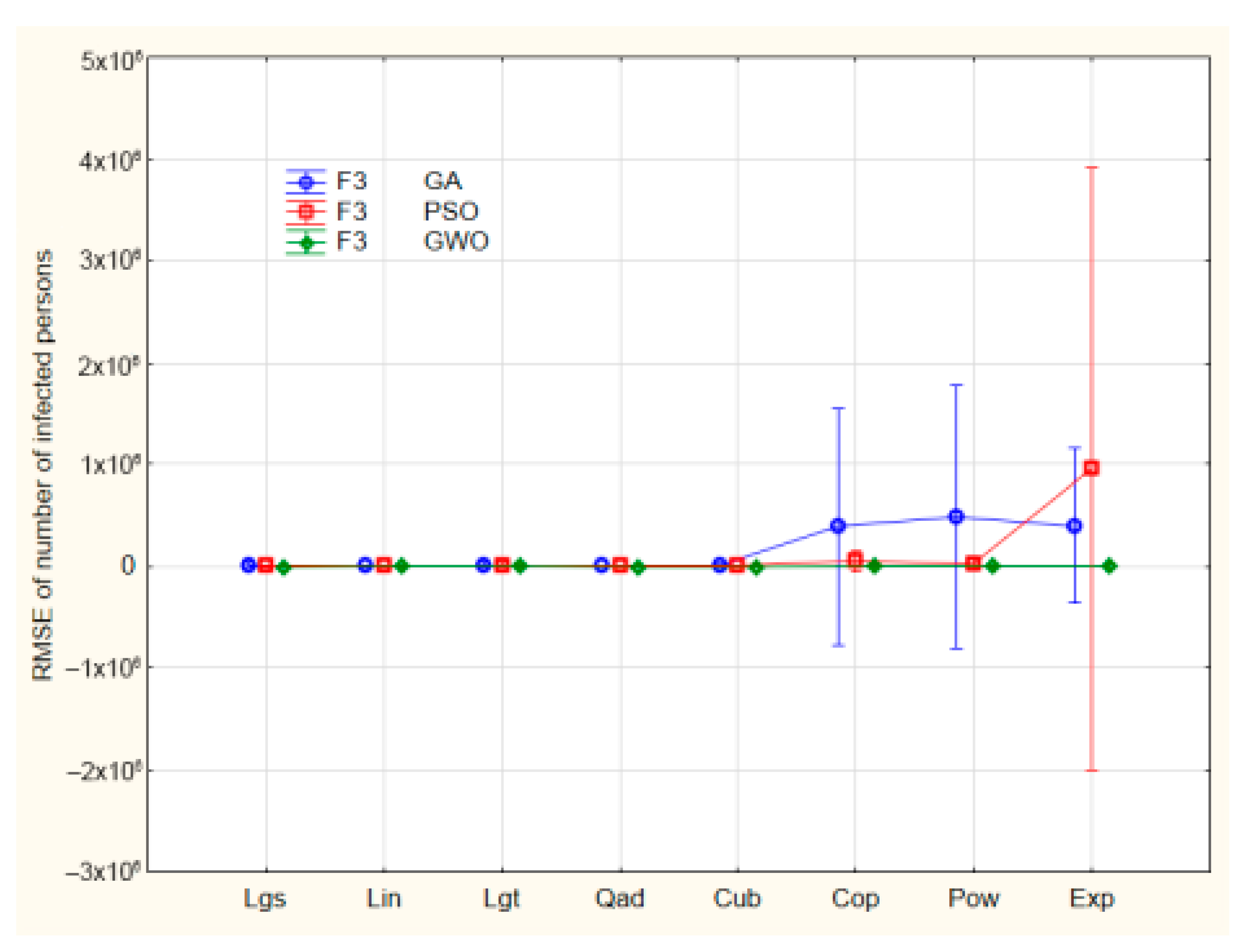
3.6. Variance Analysis of RMSEs

A prerequisite of any data analysis is to survey the data. No data preprocessing was carried out in ref. [2]. Calculation of means, median, skewness, and kurtosis could help to judge the residua normal behavior. A simple matrix plot suggests serious outliers in the data (Figure 7):
At least two outliers can be observed: 1.534 × 10⁷ (Germany, compound model and genetic algorithm) and 5.208 × 10⁷ (Italy, exponential model, and particle swarm optimization). After filtering the two outliers, a formal variance analysis (factorial ANOVA) can be completed for the RMSE data of Tables 3–10 of ref. [2]. Three factors can be decomposed: F1, countries (five levels: Italy (I), China (C), Iran (P), USA (U), Germany (G)); F2, models (eight levels; see abbreviations in the notations for Table 1); and F3, techniques of global optimum search algorithms (three levels: GA, PSO, and GWO, resolved in the notations of Table 1). One factor should be hidden as no repeated measurements are possible. The best candidate is F1 (countries) because the assumption is reasonable that the pandemic has similar trajectories in all five countries.
Neither F2 nor F3 (nor their coupling F2*F3) is significant, but the intercept only. The interaction of F2 and F3 can be seen in Figure 8.
The nonlinear models exhibit four more outliers at least. The post hoc tests (Bonferroni, Scheffé, and Tukey’s honest significant difference) show no significant differences between models and optimization algorithms either, because of the heavy outliers present. This calls for careful data preprocessing.
However, it is interesting to know whether useful information can be obtained with wrong inputs or from inappropriate starting data. The quote “garbage in, garbage out” is commonplace in modeling: if the input data used to build a model is biased (blemish), the predictions are likely to be unreliable and deceptive. On the other hand, the history of science is full of brilliant discoveries from mistaken standpoints (Columbus miscalculated the distance, Bohr’s atomic model has unrealistic postulates, Transition State Theory (TST) assumes that reactions occur at equilibrium, but frequency of collisions is set to one, Gregor Mendel’s laws of inheritance were formulated whereas he neglected observations not to cover expectations deliberately, Einstein’s theory of special relativity assumes the luminiferous ether, an invisible substance, etc.). Let us see whether wrong standpoints can lead to straightforward results.

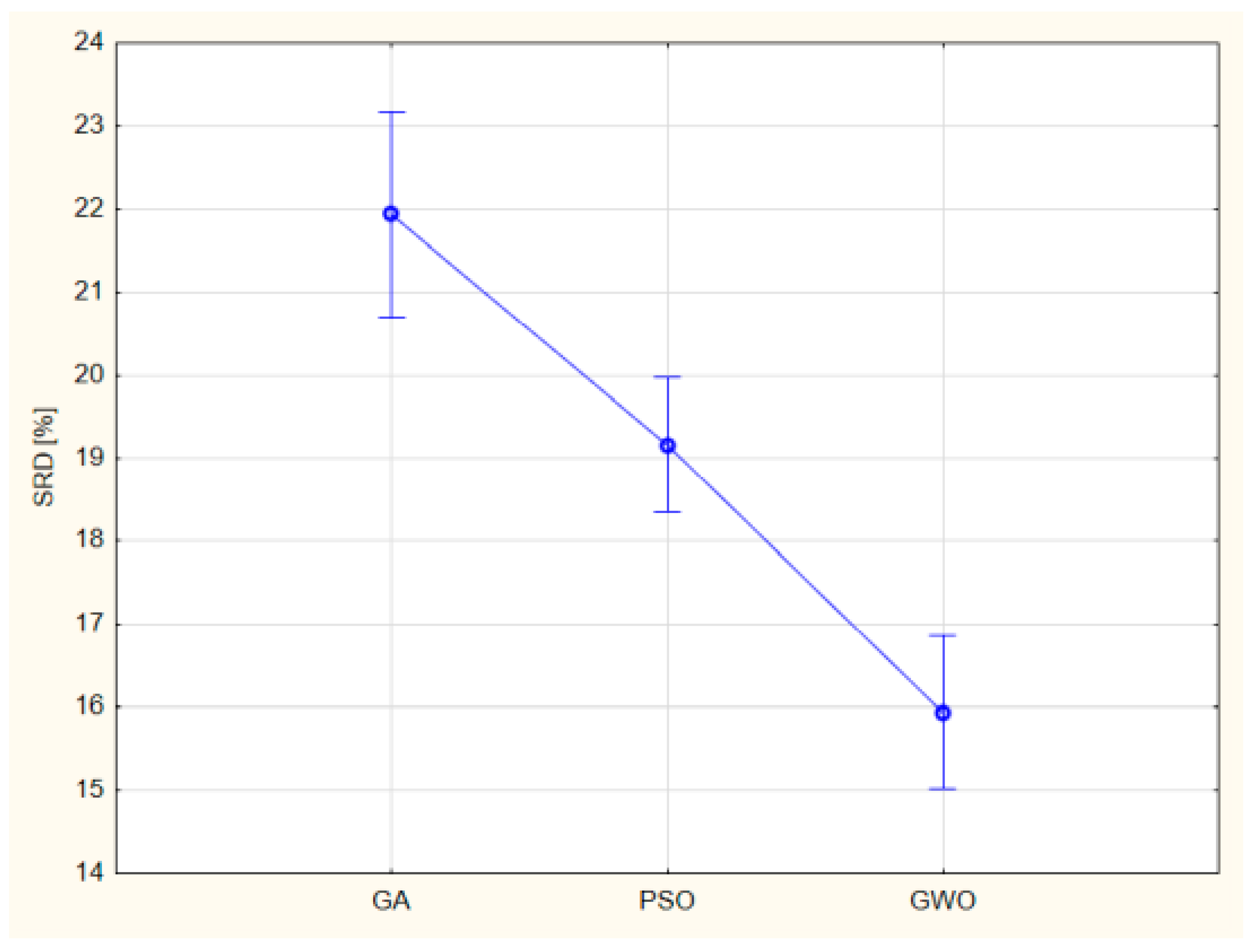
3.7. ANOVA of SRD for Algorithm Combinations

Uncertainties can be rendered to the algorithm combinations of (Figure 1 and Figure 5) if the ranking is repeated ten times leaving one row from the input matrix out at a time (each row once and only once). One new factor is introduced to factorial ANOVA: the leave-one-out (LOO) cross-validation (ten levels), whereas the countries (F1, five levels) disappear from the factors. LOO is a random factor and is, in fact, a repetition of ranking. Only robust methods are suitable, as the input data (r and RMSE of Tables 3–10 in ref. [2]) are contaminated by heavy outliers, and they are on vastly different scales. As the key step of SRD is a rank transformation, all SRD values placed on the same scale; namely, they are measured in %. All factors are significant (F2, models to be compared, F3, global optimization algorithms, and their coupling F2*F3). In Figure 9, F3 is shown only.
It should be noted that the SRD results are in (partial) accordance with the original authors’ findings: “GWO provided the highest accuracy (smallest RMSE and largest correlation coefficient) and smallest processing time compared to PSO and GA for fitting the logistic, linear, logarithmic, quadratic, cubic, power, compound, and exponential equations for all five countries. It can be suggested that GWO is a sustainable optimizer…” [2].

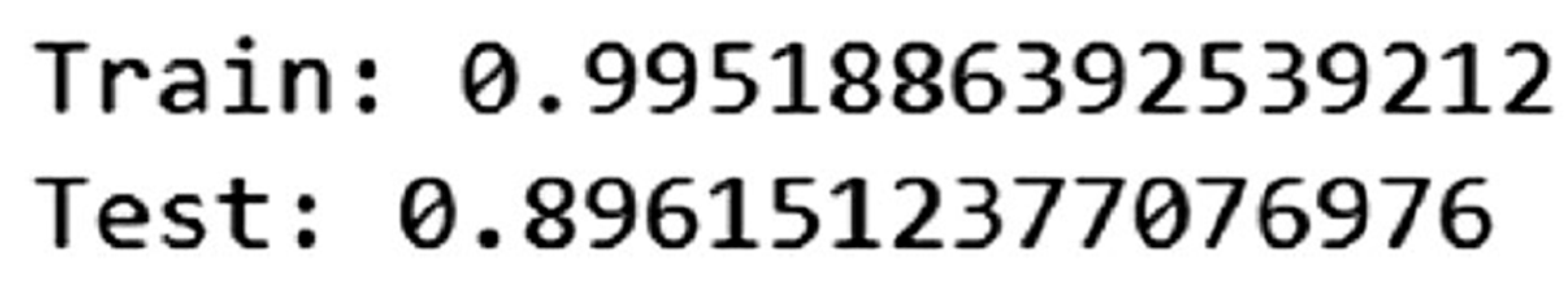
3.8. Reproducibility and Precision

A typical error is to confuse the decimal digits and value digits. Figure 10 is identical of Table 12 from ref. [2]:
Contrary to the general belief, not the decimal digits but the value digits determine the precision. The bottleneck is the minimum value digits: the end results cannot be more precise than the minimum value digits. Giving more decimal and value digits gives the false impression of obtaining and handling more precise data. A fair comparison of models is simply impossible if the fitted equations are given in different precision.

3.9. Consistent Notations, Physical Dimensions and Units

Consistent notations are required for two purposes: (i) within the manuscript (MS), they suggest that the concept was well thought-out, and the readers’ interest has also been taken into account, and (ii) outside the MS, those notations are to be used, which are common in the given (sub)field of science. Common notations enhance the understanding and citation rate. Different notations for the same variable or quantity point to sloppy work and lead to rejection eventually. Furthermore, it reveals that the authorship was not set according to the Vancouver criteria [27] (see Appendix A).
The SI standard physical dimensions are as follows (corresponding symbols are in brackets): time (T), length (L), mass (M), etc. The time is widely and unambiguously denoted by “t”, or “T”; the authors of ref. [2] use x, without any reason.
“Scalars are denoted by lower case letters x, and vectors… as bold lower-case letters: x = [x1, x2,… xn]. Matrices are denoted by bold capital letters M,…” [40].
Contrary to the common notations the authors use capital letters with arrows on the top for vectors ( X ) and indexed scalars for the same x (time) variable, units are not given.
Even worse, the match of x would be y, but the authors of ref. [2] used either R or Es and T as estimated and target values in their Equations (6)–(13) and Equation (14), respectively. Moreover, Equations (14) and (23) should be identical according to the explanation, yet the left-hand sides of the equations are different (MSE and RMSE, respectively). A summa is missing from Equation (14) and an index (i) is missing from both.
Consistency within a document or a specific context is crucial. If you are writing or editing a document, it is advisable to pick one form and stick with it throughout the MS to maintain consistency.
The correlation coefficient is a dimensionless quantity, hence its popularity: it is suitable for comparing quantities measured on different scales. In contrast, mean squared error and residual error have physical dimensions and, consequently, units. Ref. [2] never mentions physical dimension and [units], e.g., course of infection [number of infected persons], time [days].

3.10. Data Preprocessing

It is also called data curation, descriptor thinning, etc. Data reduction is unsupervised, it involves the elimination of constant and near-constant variables [41]. Similarly, highly correlated variables carry the same or highly similar information. One of them should be discarded from the input variables [41]. Even a threshold can be found by optimization [42]. Practical advice can be found in ref. [43]. No such activity has been reported in ref. [2]. Outliers can deteriorate the original distribution; their removal is also essential. Alternatively, robust methods diminish their effects; see Section 3.7.
A superficial glance at Figure 2 suggests an orange-banana comparison. The epidemy starts at different initial times. Many zeros could deteriorate models, especially the nonlinear ones. A proper shift or alignment in data processing could eliminate this error source.
The series can be continued endlessly. As our aim was to help scientists not committing such mistakes, a table was collected in binary form and color coding in the next section.

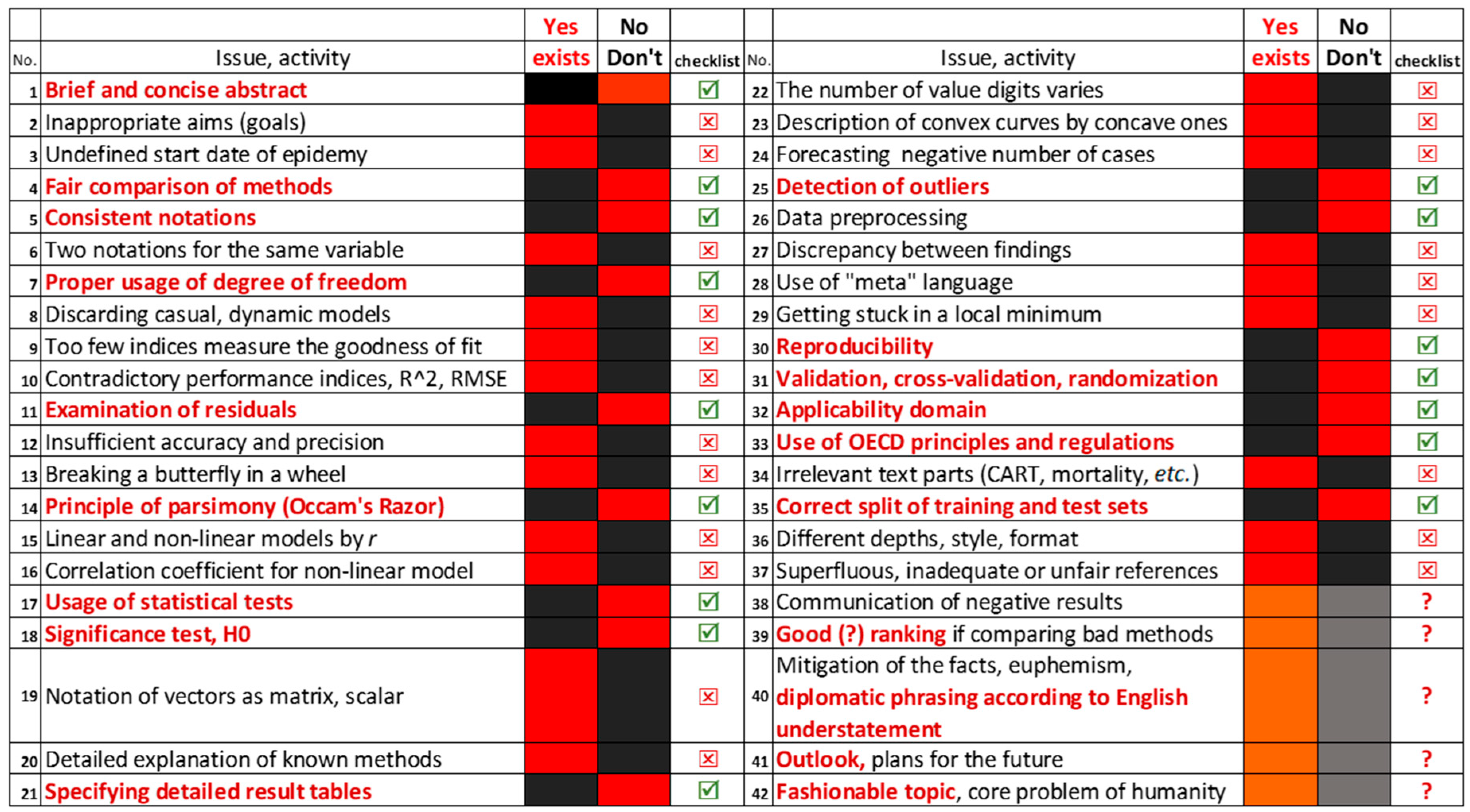
3.11. Orientation Table (Checklist)

Frequent errors committed during modeling are collected in Figure 11, apropos of ref. [2], but with general relevance.
The columns yes (exists) and no (don’t exist) correspond to ref. [2]. The green symbol means ‘required activity in general’ in any modeling paper and the red symbol means a forbidden one. Any activity in column 2 can be formulated as a question in abbreviated form, e.g., line No. 32 can be asked fully: Have the authors defined the applicability domain for which a prediction is feasible? The red color in bold indicates that the activity is required (essential), while the red field in the no (don’t exist) column indicates that this issue is missing from ref. [2], though it should be present. Similarly, a black text in column 2 indicates a mistaken standpoint, e.g., line No. 12 can be formulated as such: Was the accuracy and precision insufficient to a given problem? The red field shows in the yes (exists) column that ref. [2] failed in this respect. The symbol in the fifth and the last columns advise against such usage. A question of line 3 can be written in general form: Does the start of any time evolution (decay) set properly? Can an inhibition period be assumed?
All issues can be transferred to a question similarly. I admit the enumeration of errors is not complete and the issues have some redundancies. The wording of lines 15 and 16 are similar; line 15 objects to equal usage of correlation coefficient for linear and nonlinear models, whereas line 16 concentrates on the abuse of correlation coefficient for nonlinear ones.
The orange and gray marking indicates the advantageous and disadvantageous character of the same issue according to the intention of the writer. Mitigation or even falsifying the facts are far away from science, whereas diplomatic formulation is warranted. Further on, I concentrate fairly on the recommended practices.

4. Recommendations

There are epistemological reasons for there being no flawless scientific article or manuscript. Even the most brilliant mind (or team) has limited rationality! Therefore, a 100% error-free manuscript cannot be expected. One crucial error in Figure 11 can lead to a rejection right away. However, a 5% error is tolerable in most cases, i.e., the MS can be accepted with minor revision. If the errors achieve a critical level, say 50%, the MS cannot be accepted in its present form. A major revision is suggested above the 25% (but below 50%) error level. A revision is not adequate above the 75% level.
In any case, one should strive to produce a manuscript with a minimal number of errors. After having produced more than 1500 detailed and competent reviews and handled many hundreds of papers as an editor, the following experiences, errors, and guidelines on how to avoid misleading practices are gathered below concentrating on instances not covered in the guides of authors.

4.1. Reproducibility

A scientific paper should be fully reproducible with a detailed description of the applied methods and all datasets should be provided, or eventually, should be retrievable.

4.2. Precision

The manuscript should be carefully written to convey confidence and care. Consistent notations and correct usage of terms can help a lot. The numerical precision is determined by value digits and not by decimal digits. As the old adage says: It is not enough to be precise, you also have to appear so, e.g., Latin words and abbreviations should be set in Italics including c.f., et al., post hoc, in situ, etc.

4.3. Validation

The findings should always be validated. Many options are available in the modeling field: (i) The randomization test (y-scrambling or permutation test) is described in ref. [44]. (ii) There are many variants of cross-validation: row wise, pattern wise [45], Venetian blinds, contiguous blocks, etc. [46]. The variants should also be disclosed to obtain reproducible results [47], including proper usage of the various terms: leave-one-out, leave-many-out, k-fold-, jackknife, and bootstrap with and/or without return in resampling. (iii) Double cross-validation [48] and even repeated double cross-validation [49]. Some investigations clearly favor cross-validation over a single external one [50,51].

4.4. Training-Test Set Splits

A single split external test can by no means be considered ground truth. On the contrary, single split and external validation are different [52]. Multiple external testing is advised [29]. The advocated practice by statisticians is to divide the data set into three parts: part I is to be used for model building (variable selection); part II is for the calibration of parameters of the built model; and part III is reserved for testing the goodness of predictions [53]. Many authors combine parts I and II and carry out cross-validation. Cross-validation is perhaps the most widely used method for estimating prediction error: “Overall, five- or tenfold cross-validation are recommended as a good compromise” [54].
The Kennard–Stone algorithm [55] is frequently applied to split training and test sets based on the Euclidean distance between data points. The test set is approximately uniformly spaced i.e., mirrors the training set. However, it provides overoptimistic prediction error as compared to random selection.
There are some “beatific” ratios of training and test sets, e.g., 80%, see Figure 10 in ref. [56], or 50% (half sample cross-validation has advantageous features [57]).
The optimum depends on the objective; Kalivas et al. have recommended the selection of harmonious (and parsimonious) models [58] and suggest better models for ridge regression over principal component regression (PCR) and partial least squares regression (PLSR) contrary to the extended simulation results of ref. [7] and to the general belief. In any case, PCR and PLSR have the smallest gap in performance parameters of calibration and prediction; see Figure 2 in ref. [59].

4.5. Allocation

The fact that the allocation problem cannot be separated from performance parameters has only now become the focus of interest [60,61]. Again, different optima can be found by changing the performance parameters and the way to place the points to be measured within the datasets.
The only reasonable conclusion is that the best model(s) differs from dataset to dataset [51,62] and the optimization should be completed several times. There must not be a problem with today’s computer facilities in most cases. Therefore, multicriteria decision making (Pareto optimization) is a feasible choice considering the number of factors (algorithms, performance parameters, allocation, validation variant, etc.). Todeschini et al. have already defined a multicriteria fitness function to eliminate bad regression models [63]. The number of performance criteria is steadily increasing [20,63]. While it was not its original purpose, it turned out that the sum of ranking differences (SRD) realizes a multicriteria optimization [25,51]. Hence, SRD is recommended as the ultimate tool for model comparison, ranking and grouping models, performance parameters, and other factors. SRD is also suitable to be coupled with ANOVA, hence decomposing the effects of factors [47].

4.6. Terminology

The applied terms and expressions should be explained, all abbreviations should be resolved at the first mention, and one should not use the terms in the wrong context.

4.7. Title

It should be brief and concise (without not resolved abbreviations); definite articles are not to be used.

4.8. Abbreviations

They should not be used in titles (of figures and tables, as well), in highlights, abstracts, summaries, and conclusions. Numerous abbreviations make the MS unreadable, though a list of terms, notations, and abbreviations might be of help.

4.9. References

As a rule of thumb, never cite a paper (book chapter, etc.) if you have not read it to the full extent. The references should always be retrievable, preferably in English. Personal communication can only be accepted if the cited person provides written consent; even then, the year should be indicated. Avoid the usage of “manuscript in preparation”, or “submitted”. “Accepted” or “in press” is OK, if the source title, link, and DOI are also given.

4.10. Language

The English usage should be understandable for all. English uses the word order strictly: Object–predicate(verb)–subject–adverb of manner–locative–adverb of time. An adverb of time might be placed in very long sentences at the beginning and a comma should be used after that.

4.11. Out of Scope

The audience is not selected properly in most cases. One can imagine that in another scientific field, the results are useful and welcomed. Chasing citations and impact factors is not advisable. A proper journal leads to more understanding if the aimed audience is adequate.

4.12. Novelty

It is also connected to experimental design, but the latter is rarely considered novel in modeling journals. Nowadays, non-novelty is not a legitimate reason for rejection, if we exclude plagiarism and self-plagiarism, as well.

4.13. Note Added in Proof

Two highly relevant papers appeared while composing this article. Both are about forecasting and its validation. An alternative estimator of the out-of-sample loss was proposed using affine weights with some superior performances (it outperforms the conventional estimator in terms of sampling variability) [64]. The second one concentrated on model selection criteria: “models of different complexity may be favored, with possible negative effects on the forecasting accuracy” [65].
Back to the philosophy, Michael Crichton, the most effective promoter of science of our time, wrote [66]: “Most kinds of power require a substantial sacrifice by whoever wants the power… You must give up a lot to get it… It is literally the result of your discipline… by the time someone has acquired the ability to kill with his bare hands, he has also matured to the point where he won’t use it unwisely. So that kind of power has a built-in control. The discipline of getting the power changes you so that you won’t abuse it. But scientific power is like inherited power: attained without discipline. You read what others have done and you take the next step. You can do it very young. You can make progress very fast. There is no discipline lasting many decades. There is no mastery: old scientists are ignored. There is no humility before nature. There is only…make-a-name-for-yourself-fast philosophy… No one will criticize you. No one has any standards. They are all trying to do the same thing: to do something big, and do it fast. And because you can stand on the shoulders of giants, you can accomplish something quickly. You don’t even know exactly what you have done, but already you have reported it…”.
The words set in italics above refer to the Ortega hypothesis which says that average or mediocre experimental scientists contribute substantially to the advancement of science [67]. Unfortunately, the false Ortega hypothesis spread and proliferated based on citation count [68] and I fully agree with the final conclusion of ref. [68]: “…the importance of correction work in science cannot be overestimated: after all, the validity of the information disseminated must be regarded as more important than the speed of the dissemination”.
Unfortunately, artificial intelligence (AI) will enhance the speed and superficial summary of the expenses of validity, correctness, and precision.

5. Summary and Conclusions

This work enumerates the most frequent errors of statistical modeling on the pretext of a prototype paper (ref. [2]). Proper usages of performance parameters (merits) are enumerated and the role of degrees of freedom is emphasized. Correct ways of model discrimination are also pointed out including the comparison of linear and nonlinear models alike. Moreover, a multicriteria decision-making process has been completed to compare the combinations of modeling equations and optimization algorithms using the sum of ranking differences. Variance analysis revealed that heavy outliers were present and accentuates the importance of data preprocessing. The number of value digits determines the precision of the models. Finally, a detailed checklist was composed to help scientists avoid errors committed frequently during the modeling process.
One should keep the standards of scientific investigations (e.g., Figure 11). The ethical command prescribes that erroneous practice should be revealed and corrected, and its propagation banned.
Manuscript rejection should be the default if the results, discussion, and conclusions contradict each other or if a certain level (number) of errors is found.
Reviewers should be selected carefully from the expert pool; short reports or any sign of not reading the full manuscript should lead to being banned from the decision process and from further reviewing.
Science embodies the universal essence of humanity; let us not diminish its value by chasing after articles and citations. Our pursuit should be deeper and more meaningful.

6. Other Approaches (Outlook, Perspective)

One of the reviewers pointed out that “article [2] … is by far not representative of machine learning literature”. This statement is certainly true. So many errors cannot usually be found in a single article; that is why ref. [2] was selected as a prototype case. On the other hand, the ML literature is full of correct applications of algorithms, even if the terminology is not yet fully matured. Ref. [31] provides a free downloadable scheme where machine learning involves all modeling techniques including simple linear regression. Others confuse ANN and deep learning or big data. Personally, I would not classify an algorithm in the category of ML if the maximum likelihood solution exists in a closed form, even if the amount of data is big.
Akshay et al. suggest [69] the holistic view, i.e., taking into account several performance parameters (factors) instead of using one individual measure for accounting model goodness in accordance with the earlier findings [56]. One of the “performance metric, ROC Accuracy” is present in Figure 3G of ref. [69] but it does not exist; the authors mean the area under the curve of receiver operating characteristic curves (AUC ROC) at all probability. A polygon is formed when plotting the performance merits of the seven axes. Such a polygon is especially suitable for pattern recognition. Its area amalgamates multiple evaluation measures into a single score. The geometric properties of a seven-axes radar (web) plots have already been utilized and the area perimeter ratio is recommended together with the gravity point [70].
Di Lascio et al. have compared the local and global ML models systematically based on several performance parameters (MAE, RMSE, relative values of MAE, MAE with baseline correction and with MAE with random values, as well as Fisher scores for global and local models) [71]. Datasets (10) and splitting the data into train (~74%) calibration (~13%) and test (~13%) sets bestowed a reliable statistical analysis. The training set was also partitioned in a cross-validation manner. The quantification of diversity is unclear. A shift between training and test data occurred as expected and evaluated without mentioning the Tikhonov regularization and model update [72]. The Spearman rank correlation coefficient of 0.68 was claimed high, but the corresponding error level (1 minus significance) p = 0.055 suggests the opposite. Their statement is very true: “the optimum choice [local or global models] is often controversial”. The authors have not realized the conflicting character of performance merits. The number of compounds for each dataset and the applicability domains should have been given, too.
Weighted F1 score was applied as a single performance parameter (instead of accuracy), while the class balance was maintained in a prediction of profitability of European companies by four algorithms: linear discriminant analysis (LDA), k-nearest neighbor (kNN), decision tree (DT), and random forest (RF) [73]. Nested cross-validation wipes out the arbitrary splits of training and test sets. Yet, not surprisingly, the authors admit that “a complex algorithm does not always guarantee improved forecasting performance”. A factorial ANOVA of their Tables 5 to 7 exemplifies the next order: LDA = kNN > DT > RF contrary to basic knowledge (linear boundary and equal variance is a vital assumption of LDA whereas DT and RF are inherently non-linear). The superiority of DT and stochastic gradient boosting has been found over the logistic regression and professional analysts’ forecasts earlier (only one performance parameter (AUC ROC) was utilized in ref. [74].
The mainstream predictions of the COVID-19 pandemic have quickly diverted from foretelling new cases to other, sophisticated topics:
(i)
Numerous machine learning models were developed using plenty of performance measures (90–98%) to forecast the length of stay (LOS) and mortality rate of a patient admitted to hospital. Ensemble learning increases machine learning’s performance if many classifiers provide contradictory findings [75]. The detailed review enumerates data cleaning, outlier detection, standardization, handling of missing data, stratified k-fold cross-validation, encoder handling, >eight performance parameters, etc. However, the formula for the coefficient of determination is erroneous (Equation (20)), and the frequent 100% performance suggests a probable overfit [75].
(ii)
The predictive accuracy to predict the length of stay in a hospital has been compared for four machine learning algorithms: DT classifier, RF, ANN, and logistic regression [76]. While the data gathering, preprocessing, and feature selection can be assumed as appropriate, the categorization, the way of split to train and test sets, the usage of one performance merit, etc., leave a lot to be desired.
Figure 12 clearly shows the deficiencies. It provides accuracy values and not the “training and test dataset (SIC!)“ contrary to the title. The length of stay in hospital is a (quasi) continuous variable to be predicted: the classification information is missing. The 100.0% accuracy realizes an overfit on the training set; no cross-validation was made; the precision given by 16 decimal digits is overexaggerated, etc., as two numbers do not constitute a figure, and not even a table, either. The best accuracy was claimed at 89% (RF) and after hyperparameter tuning, 90% was achieved [76]. No statistical test showed whether the betterment had been significant.
(iii)
Another study [77] examined the “discrepancies” between AI suggestions and clinicians’ actual decisions on whether the patients should be treated in a spoke- or a hub center. Here, five parameters were considered: accuracy (76%), AUC ROC (83%), specificity (78%), recall (74%), and precision, i.e., positive predicted value (88%). The enigmatic formulation of conclusions—“[the code] is in line or slightly worse than those reported in literature for other AI driven tools” and “may help in selecting patients”—just means the opposite c.f., as shown in ref. [26].
(iv)
Brain features prior to the COVID-19 epidemic are useful for predicting the later emergence of distress [78]. Distress prediction was found significant by tenfold cross-validation with linear regression (brain features were employed as independent variables) [78].
The above small selection from among the plethora of ML applications for the COVID-19 epidemic and foretelling by ML methods proves the usefulness of ML techniques, and at the same time, calls for better usage of available techniques and validation. However, the real explosion in artificial intelligence has just started; ref. [79] is recommended to get acquainted with the problem. Fairness and bias have been chosen as a topic from the point of view of AI systems and the different domains (and subdomains) in AI were partitioned: general machine learning, deep learning, and natural language processing [79].

Supplementary Materials

The following supporting information can be downloaded at: https://www.mdpi.com/article/10.3390/a17010043/s1. Table S1: Frequent errors committed during modeling (checklist).

Funding

This work was supported by the Ministry of Innovation and Technology of Hungary from the National Research, Development and Innovation Fund, financed under the K type funding scheme (OTKA K 134260).

Data Availability Statement

Data are contained within the article.

Acknowledgments

The author thanks the editor(s) for the invitation.

Conflicts of Interest

The author declares no conflicts of interest.

Appendix A

According to the Vancouver criteria, the authorship should be based on all of the following four criteria:
  • Substantial contributions to the conception or design of the work; or the acquisition, analysis, or interpretation of data for the work.
  • Drafting the work or revising it critically for important intellectual content.
  • Final approval of the version to be published.
  • Agreement to be accountable for all aspects of the work in ensuring that questions related to the accuracy or integrity of any part of the work are appropriately investigated and resolved.
Further details including the usage of artificial intelligence (AI) can be found in ref. [27].

References

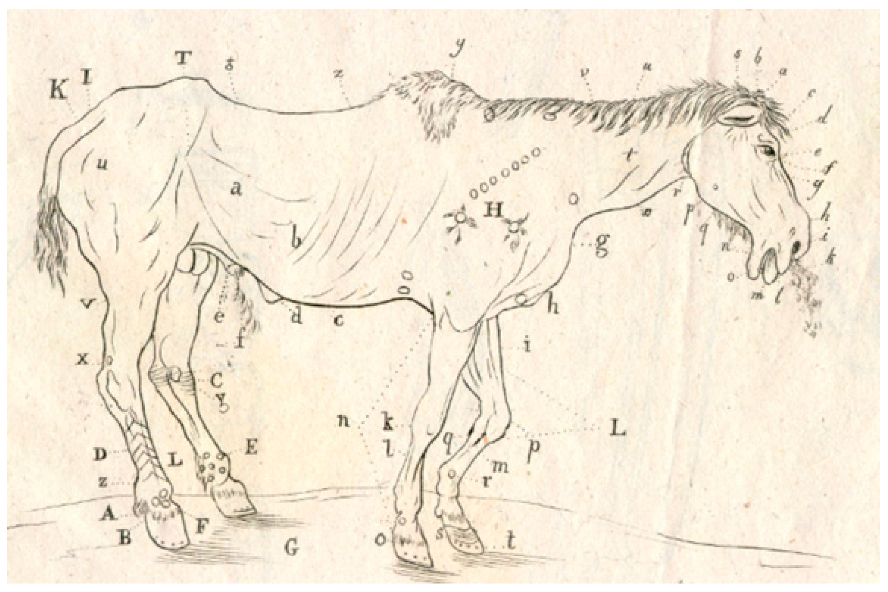
  1. Máttyus Nepomuk, J. Lótudomány Bands I and II; Pytheas Könyvmanufaktúra: Budapest, Hungary, 2008. reprint of 1845 edition. (In Hungarian) [Google Scholar]
  2. Ardabili, S.-F.; Mosavi, A.; Ghamisi, P.; Ferdinand, F.; Varkonyi-Koczy, A.R.; Reuter, U.; Rabczuk, T.; Atkinson, P.M. COVID-19 Outbreak Prediction with Machine Learning. Algorithms 2020, 13, 249. [Google Scholar] [CrossRef]
  3. Kuhn, T.S. The Structure of Scientific Revolutions; 50th Anniversary Edition; University of Chicago Press: Chicago, IL, USA, 2012; pp. 1–264. [Google Scholar]
  4. Occam’s razor. Available online: https://en.wikipedia.org/wiki/Occam%27s_razor (accessed on 29 September 2023).
  5. Breiman, L. Statistical Modeling: The Two Cultures. Stat. Sci. 2001, 16, 199–231. [Google Scholar] [CrossRef]
  6. Teter, M.D.; Newman, A.M.; Weiss, M. Consistent notation for presenting complex optimization models in technical writing. Surv. Oper. Res. Manag. Sci. 2016, 21, 1–17. [Google Scholar] [CrossRef]
  7. Frank, I.E.; Friedman, J.H. A Statistical View of Some Chemometrics Regression Tools. Technometrics 1993, 35, 109–135. [Google Scholar] [CrossRef]
  8. Gramatica, P. Principles of QSAR Modeling: Comments and Suggestions from Personal Experience. Int. J. Quant. Struct.-Prop. Relat. 2020, 5, 61–97. [Google Scholar] [CrossRef]
  9. Kirkpatrick, S.; Gelatt, C.D., Jr.; Vecchi, M.P. Optimization by Simulated Annealing. Science 1983, 220, 671–680. [Google Scholar] [CrossRef]
  10. Glover, F. Future paths for integer programming and links to artificial intelligence. Comp. Oper. Res. 1986, 13, 533–549. [Google Scholar] [CrossRef]
  11. Holland, J.H. Genetic Algorithms. Sci. Am. 1992, 267, 66–72. [Google Scholar] [CrossRef]
  12. Kennedy, J.; Eberhart, R. Particle swarm optimization. In Proceedings of the IEEE International Conference on Neural Networks—Conference Proceedings, Perth, WA, Australia, 27 November–1 December 1995; Volume 4, pp. 1942–1948, Code 44687. [Google Scholar]
  13. Dorigo, M.; Stützle, T. Ant Colony Optimization; MIT Press: Cambridge, MA, USA, 2004; pp. 1–305. [Google Scholar]
  14. Karaboga, D. An Idea Based on Honey Bee Swarm for Numerical Optimization. In Technical Report-TR06; Department of Computer Engineering, Engineering Faculty, Erciyes University: Kayseri, Türkiye, 2005; Available online: https://www.researchgate.net/publication/255638348 (accessed on 9 January 2024).
  15. Karaboga, D.; Basturk, B. Artificial Bee Colony (ABC) Optimization Algorithm for Solving Constrained Optimization Problems. In Foundations of Fuzzy Logic and Soft Computing, Proceedings of the International Fuzzy Systems Association World Congress, IFSA 2007, Cancun, Mexico, 18–21 June 2007; Melin, P., Castillo, O., Aguilar, L.T., Kacprzyk, J., Pedrycz, W., Eds.; LNAI 4529; Springer: Berlin/Heidelberg, Germany, 2007; pp. 789–798. Available online: https://link.springer.com/chapter/10.1007/978-3-540-72950-1_77 (accessed on 9 January 2024).
  16. Yang, X.S. Firefly Algorithm, Chapter 10. In Nature-Inspired Metaheuristic Algorithms; Luniver Press: Bristol, UK, 2008; pp. 81–104. Available online: https://www.researchgate.net/publication/235979455 (accessed on 9 January 2004).
  17. Yang, X.S.; Deb, S. Cuckoo search via Lévy flights. In Proceedings of the World Congress on Nature & Biologically Inspired Computing (NaBic 2009), Coimbatore, India, 9–11 December 2009; IEEE Publications: New York, NY, USA, 2009; pp. 210–214. [Google Scholar] [CrossRef]
  18. Gandomi, A.H.; Alavi, A.H. Krill herd: A new bio-inspired optimization algorithm. Commun. Nonlinear Sci. Numer. Simul. 2012, 17, 4831–4845. [Google Scholar] [CrossRef]
  19. Mirjalili, S.; Mirjalili, S.M.; Lewis, A. Grey Wolf Optimizer. Adv. Eng. Softw. 2014, 69, 46–61. [Google Scholar] [CrossRef]
  20. Héberger, K. Sum of ranking differences compares methods or models fairly. TRAC—Trends Anal. Chem. 2010, 29, 101–109. [Google Scholar] [CrossRef]
  21. Kollár-Hunek, K.; Héberger, K. Method and model comparison by sum of ranking differences in cases of repeated observations (ties). Chemom. Intell. Lab. Syst. 2013, 127, 139–146. [Google Scholar] [CrossRef]
  22. Available online: http://aki.ttk.mta.hu/srd (accessed on 5 October 2023).
  23. Héberger, K.; Kollár-Hunek, K. Sum of ranking differences for method discrimination and its validation: Comparison of ranks with random numbers. J. Chemom. 2011, 25, 151–158. [Google Scholar] [CrossRef]
  24. Sziklai, B.R.; Héberger, K. Apportionment and districting by Sum of Ranking Differences. PLoS ONE 2020, 15, e0229209. [Google Scholar] [CrossRef] [PubMed]
  25. Lourenço, J.M.; Lebensztajn, L. Post-Pareto Optimality Analysis with Sum of Ranking Differences. IEEE Trans. Magn. 2018, 54, 8202810. [Google Scholar] [CrossRef]
  26. Available online: https://www.orchidenglish.com/british-understatement/ (accessed on 5 October 2023).
  27. Available online: http://www.icmje.org/recommendations/browse/roles-and-responsibilities/defining-the-role-of-authors-and-contributors.html (accessed on 10 October 2023).
  28. Ojha, P.K.; Roy, K. Comparative QSARs for antimalarial endochins: Importance of descriptor-thinning and noise reduction prior to feature selection. Chemom. Intell. Lab. Syst. 2011, 109, 146–161. [Google Scholar] [CrossRef]
  29. Gramatica, P. External Evaluation of QSAR Models, in Addition to Cross-Validation: Verification of Predictive Capability on Totally New Chemicals. Mol. Inf. 2014, 33, 311–314. [Google Scholar] [CrossRef]
  30. Vincze, A.; Dargó, G.; Rácz, A.; Balogh, G.T. A corneal-PAMPA-based in silico model for predicting corneal permeability. J. Pharm. Biomed. Anal. 2021, 203, 114218. [Google Scholar] [CrossRef]
  31. Brownlee, J. Overfitting and Underfitting with Machine Learning Algorithms; Machine Learning Mastery: San Juan, Puerto Rico, 2019; Available online: https://machinelearningmastery.com/overfitting-and-underfitting-with-machine-learning-algorithms/ (accessed on 10 October 2023).
  32. Schwarz, G.E. Estimating the dimension of a model. Ann. Stat. 1978, 6, 461–464. [Google Scholar] [CrossRef]
  33. Akaike, H. A New Look at the Statistical Model Identification. IEEE Trans. Autom. Control 1974, 19, 716–723. [Google Scholar] [CrossRef]
  34. Draper, N.R.; Smith, I.L. Applied Regression Analysis, 2nd ed.; John Wiley & Sons: New York, NY, USA, 1981; Chapter 1; pp. 1–69. ISBN 0471170828. [Google Scholar]
  35. Rider, P.R. Introduction to Modern Statistical Methods; ASIN: B001UIDASK; John Wiley & Sons: New York, NY, USA, 1939; p. 58. [Google Scholar]
  36. Bevington, R. Data Reduction and Error Analysis for the Physical Sciences; McGraw-Hill Book Company: New York, NY, USA, 1969; Chapter 7-2, Correlation between many variables; pp. 127–133. [Google Scholar]
  37. Héberger, K. Discrimination between Linear and Non-Linear Models Describing Retention Data of Alkylbenzenes in Gas-Chromatography. Chromatographia 1990, 29, 375–384. [Google Scholar] [CrossRef]
  38. Héberger, K. Empirical Correlations Between Gas-Chromatographic Retention Data and Physical or Topological Properties of Solute Molecules. Anal. Chim. Acta 1989, 223, 161–174. [Google Scholar] [CrossRef]
  39. Bard, Y. Nonlinear Parameter Estimation; Academic Press: New York, NY, USA, 1974; pp. 269–271. [Google Scholar]
  40. Erichson, N.B.; Zheng, P.; Manohar, K.; Brunton, S.L.; Kutz, J.N.; Aravkin, A.Y. Sparse Principal Component Analysis via Variable Projection. SIAM J. Appl. Math. 2020, 80, 977–1002. [Google Scholar] [CrossRef]
  41. Todeschini, R.; Consonni, V. Molecular Descriptors for Chemoinformatics; WILEY-VCH Verlag: Weinheim, Germany; GmbH & Co. KGaA: Weinheim, Germany, 2010; Volume 2, pp. 1–252. [Google Scholar] [CrossRef]
  42. Rácz, A.; Bajusz, D.; Héberger, K. Intercorrelation limits in molecular descriptor preselection for QSAR/QSPR. Mol. Inform. 2019, 38, 1800154. [Google Scholar] [CrossRef] [PubMed]
  43. García, S.; Luengo, J.; Herrera, F. Tutorial on practical tips of the most influential data preprocessing algorithms in data mining. Knowl.-Based Syst. 2016, 98, 1–29. [Google Scholar] [CrossRef]
  44. Rücker, C.; Rücker, G.; Meringer, M. y-Randomization and Its Variants in QSPR/QSAR. J. Chem. Inf. Model. 2007, 47, 2345–2357. [Google Scholar] [CrossRef] [PubMed]
  45. Bro, R.; Kjeldahl, K.; Smilde, A.K.; Kiers, H.A.L. Cross-validation of component models: A critical look at current methods. Anal. Bioanal. Chem. 2008, 390, 1241–1251. [Google Scholar] [CrossRef]
  46. Using Cross-Validation. Available online: http://wiki.eigenvector.com/index.php?title=Using_Cross-Validation (accessed on 11 November 2023).
  47. Heberger, K.; Kollar-Hunek, K. Comparison of validation variants by sum of ranking differences and ANOVA. J. Chemom. 2019, 33, e3104. [Google Scholar] [CrossRef]
  48. Baumann, D.; Baumann, K. Reliable estimation of prediction errors for QSAR models under model uncertainty using double cross-validation. J. Cheminform. 2014, 6, 47. Available online: http://www.jcheminf.com/content/6/1/47 (accessed on 9 January 2024). [CrossRef]
  49. Filzmoser, P.; Liebmann, B.; Varmuza, K. Repeated double cross validation. J. Chemom. 2009, 23, 160–171. [Google Scholar] [CrossRef]
  50. Gütlein, M.; Helma, C.; Karwath, A.; Kramer, S. A Large-Scale Empirical Evaluation of Cross-Validation and External Test Set Validation in (Q)SAR. Mol. Inf. 2013, 32, 516–528. [Google Scholar] [CrossRef] [PubMed]
  51. Rácz, A.; Bajusz, D.; Héberger, K. Consistency of QSAR models: Correct split of training and test sets, ranking of models and performance parameters. SAR QSAR Environ. Res. 2015, 26, 683–700. [Google Scholar] [CrossRef] [PubMed]
  52. Esbensen, K.H.; Geladi, P. Principles of proper validation: Use and abuse of re-sampling for validation. J. Chemom. 2010, 24, 168–187. [Google Scholar] [CrossRef]
  53. Miller, A. Part 1.4 ‘Black box’ use of best-subsets techniques. In Subset Selection in Regression; Chapman and Hall: London, UK, 1990; p. 13. [Google Scholar]
  54. Hastie, T.; Tibshirani, R.; Friedman, J.H. Chapter 7.10 Cross-validation. In The Elements of Statistical Learning: Data Mining, Inference, and Prediction, 2nd ed.; Springer: New York, NY, USA, 2009; pp. 241–249. Available online: https://hastie.su.domains/Papers/ESLII.pdf (accessed on 9 January 2024).
  55. Kennard, R.W.; Stone, L.A. Computer aided design of experiments. Technometrics 1969, 11, 137–148. [Google Scholar] [CrossRef]
  56. Rácz, A.; Bajusz, D.; Héberger, K. Effect of Dataset Size and Train/Test Split Ratios in QSAR/QSPR Multiclass Classification. Molecules 2021, 26, 1111. [Google Scholar] [CrossRef] [PubMed]
  57. Efron, B. Estimating the Error Rate of a Prediction Rule: Improvement of Cross-Validation. J. Am. Stat. Assoc. 1983, 78, 316–331. Available online: https://www.jstor.org/stable/2288636 (accessed on 9 January 2024). [CrossRef]
  58. Kalivas, J.H.; Forrester, J.B.; Seipel, H.A. QSAR modeling based on the bias/variance compromise: A harmonious and parsimonious approach. J. Comput.-Aided Mol. Des. 2004, 18, 537–547. [Google Scholar] [CrossRef]
  59. Rácz, A.; Bajusz, D.; Héberger, K. Modelling methods and cross-validation variants in QSAR: A multi-level analysis. SAR QSAR Environ. Res. 2018, 29, 661–674. [Google Scholar] [CrossRef]
  60. Consonni, V.; Ballabio, D.; Todeschini, R. Evaluation of model predictive ability by external validation techniques. J. Chemom. 2010, 24, 194–201. [Google Scholar] [CrossRef]
  61. Tóth, G.; Király, P.; Kovács, D. Effect of variable allocation on validation and optimality parameters and on cross-optimization perspectives. Chemom. Intell. Lab. Syst. 2020, 204, 104106. [Google Scholar] [CrossRef]
  62. Roy, P.P.; Leonard, J.T.; Roy, K. Exploring the impact of size of training sets for the development of predictive QSAR models. Chemom. Intell. Lab. Syst. 2008, 90, 31–42. [Google Scholar] [CrossRef]
  63. Todeschini, R.; Consonni, V.; Mauri, A.; Pavan, M. Detecting “bad” regression models: Multicriteria fitness functions in regression analysis. Anal. Chim. Acta 2004, 515, 199–208. [Google Scholar] [CrossRef]
  64. Staněk, F. Optimal out-of-sample forecast evaluation under stationarity. J. Forecast. 2023, 42, 2249–2279. [Google Scholar] [CrossRef]
  65. Spiliotis, E.; Petropoulos, F.; Assimakopoulos, V. On the Disagreement of Forecasting Model Selection Criteria. Forecasting 2023, 5, 487–498. [Google Scholar] [CrossRef]
  66. Crichton, M. Jurassic Park; Ballantine Books: New York, NY, USA, 1990; p. 306. [Google Scholar]
  67. Ortega Hypothesis. Available online: https://en.wikipedia.org/wiki/Ortega_hypothesis (accessed on 14 November 2023).
  68. Száva-Kováts, E. The false ‘Ortega Hypothesis’: A literature science case study. J. Inform. Sci. 2004, 30, 496–508. [Google Scholar] [CrossRef]
  69. Aksha, A.; Abedi, M.; Shekarchizadeh, N.; Burkhard, F.C.; Katoch, M.; Bigger-Allen, A.; Adam, R.M.; Monastyrskaya, K.; Gheinani, A.H. MLcps: Machine learning cumulative performance score for classification problems. GigaScience 2023, 12, giad108. [Google Scholar] [CrossRef]
  70. Kollár-Hunek, K.; Heszberger, J.; Kókai, Z.; Láng-Lázi, M.; Papp, E. Testing panel consistency with GCAP method in food profile analysis. J. Chemometr. 2008, 22, 218–226. [Google Scholar] [CrossRef]
  71. Di Lascio, E.; Gerebtzoff, G.; Rodríguez-Pérez, R. Systematic Evaluation of Local and Global Machine Learning Models for the Prediction of ADME Properties. Mol. Pharm. 2023, 20, 1758–1767. [Google Scholar] [CrossRef]
  72. Kalivas, J.H. Overview of two-norm (L2) and one-norm (L1) Tikhonov regularization variants for full wavelength or sparse spectral multivariate calibration models or maintenance. J. Chemometr. 2012, 26, 218–230. [Google Scholar] [CrossRef]
  73. Belesis, N.D.; Papanastasopoulos, G.A.; Vasilatos, M.A. Predicting the Profitability of Directional Changes using Machine Learning: Evidence from European Countries. J. Risk Financ. Manag. 2023, 16, 520. [Google Scholar] [CrossRef]
  74. Chen, X.; Cho, Y.H.; Dou, Y.; Lev, B. Predicting Future Earnings Changes using Machine Learning and Detailed Financial Data. J. Account. Res. 2022, 60, 467–515. [Google Scholar] [CrossRef]
  75. Bhadouria, A.S.; Singh, R.K. Machine learning model for healthcare investments predicting the length of stay in a hospital and mortality rate. Multimed. Tools Appl. 2023. [Google Scholar] [CrossRef]
  76. Samy, S.S.; Karthick, S.; Ghosal, M.; Singh, S.; Sudarsan, J.S.; Nithiyanantham, S. Adoption of machine learning algorithm for predicting the length of stay of patients (construction workers) during COVID pandemic. Int. J. Inf. Technol. 2023, 15, 2613–2621. [Google Scholar] [CrossRef] [PubMed]
  77. Catalano, M.; Bortolotto, C.; Nicora, G.; Achilli, M.F.; Consonni, A.; Ruongo, L.; Callea, G.; Tito, A.L.; Biasibetti, C.; Donatelli, A.; et al. Performance of an AI algorithm during the different phases of the COVID pandemics: What can we learn from the AI and vice versa. Eur. J. Radiol. 2023, 11, 100497. [Google Scholar] [CrossRef]
  78. Pan, N.; Qin, K.; Yu, Y.; Long, Y.; Zhang, X.; He, M.; Suo, X.; Zhang, S.; Sweeney, J.A.; Wang, S.; et al. Pre-COVID brain functional connectome features prospectively predict emergence of distress symptoms after onset of the COVID-19 pandemic. Psychol. Med. 2023, 53, 5155–5166. [Google Scholar] [CrossRef]
  79. Mehrabi, N.; Morstatter, F.; Saxena, N.; Lerman, K.; Galstyan., A. A Survey on Bias and Fairness in Machine Learning. ACM Comput. Surv. 2021, 54, 115. [Google Scholar] [CrossRef]
Figure 1. The so-called “veterinary horse”, with all the diseases that, in practice, cannot occur in a single horse at the same time. This figure derived from ref. [1]; the letters indicate the various diseases.
Algorithms 17 00043 g001
Figure 2. Cumulative number of COVID-19 cases [number of infected persons] for five countries over 30 days from ref. [2]. The starting times and the duration of the observation period are different. Something happened around 12 February (China), which cannot be explained by the epidemic, but by political/regulatory reasons.
Algorithms 17 00043 g002
Figure 3. The eight models compared in ref. [2] aimed to find their optimal performance (prediction). The number of constants to be fitted varies between two to four and the equations cover linear and nonlinear (convex and concave) ones. The notation of R is not explained there.
Algorithms 17 00043 g003
Figure 4. The abstract of ref. [2]. Color coding: grey—preliminaries, background, and results of earlier investigations; white—filler text, without information content; turquoise—dubious meaning because of the English understatement [26]; yellow—untrue statements, not the results of present investigations or in contradiction with the discussion section.
Algorithms 17 00043 g004
Figure 5. Sum of ranking differences (SRD) groups the algorithm combinations. (SRD values are scaled between 0 and 100, the smaller the better). Scaled SRD values are plotted on the x and left y axes, the right y axis shows the cumulated relative frequencies of random ranking: black curve. The probability ranges are also given as 5% (XX1), Median (Med), and 95% (XX19). The explanation of capital letters A, B, … F can be found in Table 1.
Algorithms 17 00043 g005
Figure 6. (Figure 10 from ref. [2]): performance of all models of Figure 3 was compared for description of epidemic data of Germany by using GWO for minimum search.
Algorithms 17 00043 g006
Figure 7. Matrix plot for global minimum search algorithms (RMSE values from data of Tables 3–10 in ref. [2]). Histograms are seen in the plots of the diagonal (y axes show the frequencies, whereas x axes the RMSE values), RMSE values can be found on the y and x axes alike for the off-diagonal plots. Blue circles stand for the points of RMSE values. GA, PSO, and GWO are abbreviations for optimization algorithms. The linear regression lines (red) are based on one (or two) outlier(s). The presence of outliers is obvious.
Algorithms 17 00043 g007
Figure 8. Decomposition of models (in Figure 3) and global optimization methods. For abbreviations in x axis see the notations of Table 1.
Algorithms 17 00043 g008
Figure 9. Significant differences between global optimization algorithms: genetic algorithm is the worst; particle swarm optimization is somewhat better and grey wolf optimization is the best option as follows from SRD analysis of r and RMSE data of Tables 3–10 in ref. [2].
Algorithms 17 00043 g009
Figure 10. (Table 12 in ref. [2]): yellow markings show the different number of value precisions. Meaning of superscripts: A—2 value-, 3 decimal digits; B—3 value-, 2 decimal digits; C—3 value-, 3 decimal digits; D—4 value-, 2 decimal digits; E—5 value-, 2 decimal digits; F—6 value-, 2 decimal digits; G—7 value-, 2 decimal digits; H—7 value-, 3 decimal digits.
Algorithms 17 00043 g010
Figure 11. Important issues while writing a manuscript simplified to binary “yes” and “no” answers. Black text in column 2 means a negative contribution, whereas red (bold) means a positive one (orange—grey fields indicate not unambiguous meaning, non-binary answers). This figure is available as Supplementary Material in MS Excel format for free extension and individual checks.
Algorithms 17 00043 g011
Figure 12. Figure 12 from ref. [76] entitled “Train and Test Dataset for Random Forest”. With permission of Springer Nature, License Number 5705470540586.
Algorithms 17 00043 g012
Table 1. Contains the grouping pattern of algorithm combinations (color coding corresponds to that of Figure 5).
ClusterAbbreviationClusterAbbreviation
ALgs_GWOBPow_PSO
ACop_GWOBQad_GA
AExp_GWOCQad_GWO
BLgs_PSOCCub_PSO
BLin_GACCop_PSO
BLin_PSOCPow_GWO
BLin_GWOCExp_PSO
BLgt_GADLgs_GA
BLgt_PSOEQad_PSO
BLgt_GWOECop_GA
BCub_GWOFCub_GA
BPow_GAFExp_GA
Notations: Lgs—logistic, Lin—linear, Lgt—logarithmic, Qad—quadratic, Cub—cubic, Cop—compound, Pow—power, and Exp—exponential equations; after underscore: GA—genetic algorithm, PSO—particle swarm optimization, GWO—grey wolf optimizer.
Disclaimer/Publisher’s Note: The statements, opinions and data contained in all publications are solely those of the individual author(s) and contributor(s) and not of MDPI and/or the editor(s). MDPI and/or the editor(s) disclaim responsibility for any injury to people or property resulting from any ideas, methods, instructions or products referred to in the content.

