Numerical Algorithms in III–V Semiconductor Heterostructures

Abstract

In the current research, we consider the solution of dispersion relations addressed to solid state physics by using artificial neural networks (ANNs). Most specifically, in a double semiconductor heterostructure, we theoretically investigate the dispersion relations of the interface polariton (IP) modes and describe the reststrahlen frequency bands between the frequencies of the transverse and longitudinal optical phonons. The numerical results obtained by the aforementioned methods are in agreement with the results obtained by the recently published literature. Two methods were used to train the neural network: a hybrid genetic algorithm and a modified version of the well-known particle swarm optimization method.

1. Introduction

Due to the increasing needs for high-quality nanostructures, several advanced growth techniques, e.g., molecular beam epitaxy (MBE), metal organic chemical vapor deposition (MOCVD), and Stranski–Krastanow growth [1], have been used to manufacture qualitative quantum structures constructed with dielectric materials. In polar dielectric crystals, phonon polaritons, which are the result of the coupling of optical phonons with an electromagnetic field (photon), are of crucial importance in low-dimensional structures (LDS) excitation processes. During recent decades, several theoretical and experimental results have been reported in research areas like surface phonon polaritons, polariton–electron interactions in semiconductor microcavities, phonon–polariton modes in superlattices, and polariton modes in ferroelectric/graphene heterostructure systems [2,3,4,5,6,7], among others. The studying of phonon polaritons and their coupling to electrons within a semiconductor LDS (e.g., quantum wells and superlatices) play an important role to control and enhance the quantum efficiency of infrared (IR) detectors, quantum witches (QWs), and semiconductor lasing structures, among others [8]. Furthermore, numerical methods like finite elements [9,10], direct diagonalization techniques [11], and integration methods are a few methods that have been employed to solve numerical problems in research related to phonon polariton processes. Many previous works (e.g., [3]) have used simple numerical methods to calculate the phonon polariton modes. This work suggests the application of artificial neural networks [12,13] to estimate the phonon polariton modes. More specifically, for a quantum well structure, we have calculated the interface polariton frequencies as a function of the polariton in-plane wavevector in order to describe the reststrahlen frequency bands between the frequencies of the transverse and longitudinal optical phonons.

Neural networks have been used in a variety of cases, such as problems from physics [14,15,16], as solutions of differential equations [17,18], agriculture problems [19,20], chemistry problems [21,22,23], problems related to economics [24,25,26], medicine problems [27,28], etc. Artificial neural networks are usually formulated as functions $N(\overrightarrow{x},\overrightarrow{w})$. Vector $\overrightarrow{x}$ represents the input pattern and vector $\overrightarrow{w}$ is called the weight vector. As suggested in [29], the neural network can be expressed as the following summation:

$$N\left(\overrightarrow{x},\overrightarrow{w}\right)=\sum _{i=1}^K{w}_{(d+2)i-(d+1)}\sigma \left(\sum _{j=1}^d{x}_j{w}_{(d+2)i-(d+1)+j}+w_{(d+2)i}\right)$$

(1)

Parameter K stands for the number of processing nodes, and parameter d represents the dimension of the input pattern. The used function $\sigma \left(x\right)$ is known as sigmoid function in the relevant literature and is formulated as

$$\sigma \left(x\right)=\frac{1}{1+exp(-x)}$$

(2)

Recently, artificial neural networks have been applied to some solid state physics problems, such as identification of quantum phase transitions [30], solving of the electronic Schrödinger equation [31], heat transfer problems [32], metal additive manufacturing [33], etc.

The sections of this article are organized as follows: in Section 2, the objective problem and the methods used to tackle it are presented in detail; in Section 3, the experimental results are outlined, and, finally, in Section 4, some conclusions from the application of the optimization methods are discussed thoroughly.

2. Materials and Methods

This section will begin by presenting the theoretical background of the present study and the approximation model used, and continue by presenting the computational techniques used to train the model.

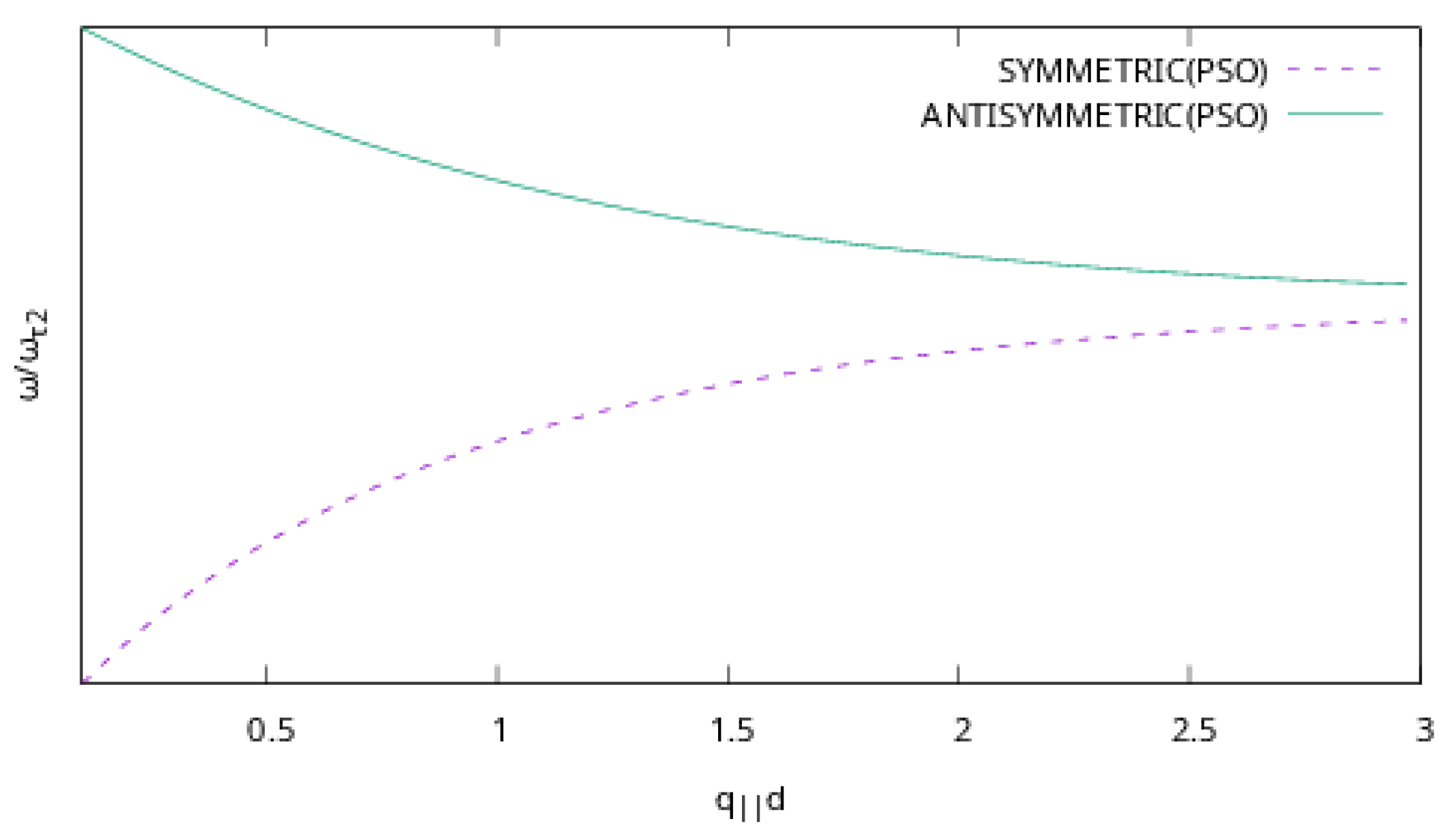
2.1. Theory

In a semiconductor structure, the electron–polariton Hamiltonian can be described by the following formula:

$$H=H_0+H_{free}+H_{int}$$

(3)

where the unperturbed electron Hamiltonian is approximated (effective mass approximation) to

$$H_0=\frac{p^2}{2m^{*}}+V_{CB}$$

(4)

with $V_{CB}$ the conduction band profile, p the electron momentum, and $m_{*}$ the electron effective mass.

The free field Hamiltonian has the form

$$H_{free}=\frac{{ϵ}_o}{2}\sum _{\omega }\left(\int \frac{\partial \left(\omega ϵ\left(\omega \right)\right)}{\partial \omega }{E}^2+c{B}^2\right)$$

(5)

where $ϵ\left(\omega \right)$ is frequency-dependent, ${ϵ}_o$ is the permittivity of free space, and c is the velocity of light in vacuum. The electric and the magnetic field, related to the polariton, are respectively denoted by E and B. By ignoring higher-order processes, the electrons interact with polaritons via the interaction Hamiltonian

$$H_{int}=\frac{e}{m^{*}}\mathbf{A}·\mathbf{p}$$

(6)

where $\mathbf{A}$ is the vector potential that describes the polaritons.

Let us consider a double heterostructure constructed with GaAs/AlAs with a well width of d. The dielectric functions to describe the interface Fuchs–Kliewer (FK) polaritons in the heterostructure are provided by [6]

$${ϵ}_i={ϵ}_{\infty ,i}\frac{{\omega }^2-{\omega }_{L,i}^2}{{\omega }^2-{\omega }_{T,i}^2}$$

(7)

where ${ϵ}_{\infty ,i}$ is the high-frequency dielectric constant, ${\omega }_{L,i}$ and ${\omega }_{T,i}$ are the zone center LO and TO optical frequencies of the i-th material. The symmetric and the antisymmetric interface mode dispersion relations are, respectively, provided by the following equations

$$\frac{{ϵ}_2\left(\omega \right)q_1}{{ϵ}_1\left(\omega \right)q_2}=-coth\left(\frac{q_{2}d}{2}\right)$$

(8)

$$\frac{{ϵ}_2\left(\omega \right)q_1}{{ϵ}_1\left(\omega \right)q_2}=-tanh\left(\frac{q_{2}d}{2}\right)$$

(9)

Wavevectors $q_i$ and the in-plane wavevector $q_{\left|\right|}$ are provided by

$$q_i^2=q_{\left|\right|}^2-{\omega }^2{ϵ}_i\left(\omega \right)/c^2$$

(10)

Hence, by combining Equations (8) and (9), the following optimization problem can be formulated:

$$min\sum _{q_{\left|\right|}=t_0}^{t_1}\left({\left(\frac{{ϵ}_2\left({\omega }_1\right)q_1}{{ϵ}_1\left({\omega }_1\right)q_2}+coth\left(\frac{q_{2}d}{2}\right)\right)}^2+{\left(\frac{{ϵ}_2\left({\omega }_2\right)q_1}{{ϵ}_1\left({\omega }_2\right)q_2}+tanh\left(\frac{q_{2}d}{2}\right)\right)}^2\right)$$

(11)

Equation (11) should be minimized with respect to independent variables ${\omega }_1,{\omega }_2$, and parameter $q_{\left|\right|}$ varies from $t_0$ to $t_1$. In the current implementation, the artificial neural networks $N_1\left(q_{\left|\right|},\overrightarrow{w}\right),N_2\left(q_{\left|\right|},\overrightarrow{w}\right)$ were used in place of variables ${\omega }_1,{\omega }_2$. Using Equation (1) with $d=1$, the final form of used neural network is

$$N\left(q_{\left|\right|},\overrightarrow{w}\right)=\sum _{i=1}^K{w}_{3i-2}\sigma \left(q_{\left|\right|}{w}_{3i-1}+w_{3i}\right)$$

(12)

where K denotes the number of weights for the neural network. Hence, the optimization problem of Equation (11) is transformed to the following one:

$$min\sum _{q_{\left|\right|}=t_0}^{t_1}\left({\left(\frac{{ϵ}_2\left(N_1(q_{\left|\right|},\overrightarrow{w_1}\right)q_1}{{ϵ}_1(N_1\left(q_{\left|\right|},\overrightarrow{w_1}\right)q_2}+coth\left(\frac{q_{2}d}{2}\right)\right)}^2+{\left(\frac{{ϵ}_2(N_2\left(q_{\left|\right|},\overrightarrow{w_2}\right)q_1}{{ϵ}_1(N_2\left(q_{\left|\right|},\overrightarrow{w_2}\right)q_2}+tanh\left(\frac{q_{2}d}{2}\right)\right)}^2\right)$$

(13)

For experimental purposes, the interval $[t_0,t_1]$ is divided into $NP$ equidistant points, forming the set $X=[x_0=t_0,x_1,\dots ,x_{NP}=t_1]$, and hence the following equation will be minimized:

$$min\sum _{i=0}^{NP}\left({\left(\frac{{ϵ}_2\left(N_1(x_i,\overrightarrow{w_1}\right)q_1}{{ϵ}_1(N_1\left(x_i,\overrightarrow{w_1}\right)q_2}+coth\left(\frac{q_{2}d}{2}\right)\right)}^2+{\left(\frac{{ϵ}_2(N_2\left(x_i,\overrightarrow{w_2}\right)q_1}{{ϵ}_1(N_2\left(x_i,\overrightarrow{w_2}\right)q_2}+tanh\left(\frac{q_{2}d}{2}\right)\right)}^2\right)$$

(14)

In the following subsection, two methods will be analyzed that were used to optimize Equation (14) with respect to weight vectors $\overrightarrow{w_1},\overrightarrow{w_2}$.

2.2. The Used Genetic Algorithm

The first algorithm used to optimize the problem of Equation (14) is a modification of the genetic algorithm. Genetic algorithms suggested by John Holland [34] are inspired by biology, and the algorithm initiates by formulating an initial population of potential solutions for any optimization problem. These solutions are also called chromosomes. The chromosomes are iteratively altered using the biologically inspired operations of selection, crossover, and mutation [35]. Genetic algorithms have been used in a variety of optimization problems, such as aerodynamic optimization [36], steel structure optimization [37], image processing problems [38], etc. Also, they have been used as the training methods of neural networks in a variety of papers, such as the paper of Leung et al. [39] used to estimate the topology of neural networks. Also, they have been used to construct neural networks for daily rainfall runoff forecasting [40], evolving neural networks for the deformation modulus of rock masses [41], etc.

The steps of the modified genetic algorithm are outlined below.

• Initialization Step

  (a)

  Set with $N_C$ the total number of chromosomes.

  (b)

  Set with $N_G$ the total number of generations allowed.

  (c)

  Define with K the number of weights for the neural networks.

  (d)

  Produce randomly $N_C$ chromosomes. Every chromosome consists of two equal parts. The first half represents the parameters of the artificial neural network $N_1(x,\overrightarrow{w_1}$ and the second half represents the parameters of the artificial neural network $N_2(x,\overrightarrow{w_2}$. The size of each part is set to 3K, where K is the number of weights.

  (e)

  Set as $p_s$ the selection rate, with $p_s\le 1$.

  (f)

  Set as $p_m$ the mutation rate, with $p_m\le 1$.

  (g)

  Set iter = 0.

• Fitness calculation Step

  (a)

  For $i=1,\dots ,N_G$, do

  • Calculate the fitness $f_i$ of every chromosome $g_i$. The chromosome consists of two equal parts. The first part (parameters in range $[1\dots 3K]$ is used to represent the parameters of the artificial neural network $N_1$ and the second part (parameters in range $[3K+1\dots 6K]$ ) represents the parameters of the artificial neural network $N_2$. The calculation of the fitness has the following steps:
    • Set $w_1=g_i[1\dots 3K]$, the first part of chromosome $g_i$
    • Set $w_2=g_i[3K+1\dots 6K]$, the second part of chromosome $g_i$
    • Set $f_i$ the value for Equation (14)

  (b)

  EndFor

• Genetic operations step

  (a)

  Selection procedure. After sorting according to the fitness values, the first $\left(1-p_s\right)\times N_C$ chromosomes with the lowest fitness values are copied to the next generation and the rest are replaced by offsprings produced during the crossover procedure.

  (b)

  Crossover procedure: Two new offsprings $\tilde{z}$ and $\tilde{w}$ are created for every selected couple of $(z,w)$. The selection of $(z,w)$ is performed using the tournament selection. The new offsprings are produced according to the following:

  $$\begin{array}{ccc}\hfill \widetilde{z_i}& =& a_i{z}_i+\left(1-a_i\right)w_i\hfill \\ \hfill \widetilde{w_i}& =& a_i{w}_i+\left(1-a_i\right)z_i\hfill \end{array}$$

  (15)

  The value $a_i$ is a random number, where $a_i\in [-0.5,1.5]$ [42].

  (c)

  Perform the mutation procedure: For every element of each chromosome, a random number number $r\in \left[0,1\right]$ is drawn. If $r\le p_m$, then this element is altered randomly.

• Termination Check Step

  (a)

  Set  $iter=iter+1$

  (b)

  The termination rule used here was initially proposed in the work of Tsoulos [43]. The algorithm computes the variance of the best-located fitness value at every iteration. If no better value was discovered for a number of generations, then this is a good evidence that the algorithm should terminate. Consider $f\left(g_{\mathrm{best}}\right)$ as the best fitness of the population and ${\sigma }^{\left(\mathrm{iter}\right)}$ as the associated variance at generation iter. The termination rule is formulated as

  $$\mathrm{iter}\ge N_G\mathrm{OR}{\sigma }^{\left(\mathrm{iter}\right)}\le \frac{{\sigma }^{\left(\mathrm{klast}\right)}}{2}$$

  (16)

  where $\mathrm{klast}$ is the last generation where a new minimum was found.

  (c)

  If the termination rule is not satisfied, go to step 2.

• Local Search Step

  (a)

  Set $g_{\mathrm{best}}$ the best chromosome of the population.

  (b)

  Apply a local search procedure $C^{*}=\mathcal{L}\left(g_{\mathrm{best}}\right)$ to the best chromosome. In the current implementation, the BFGS method published by Powell [44] was used as a local search procedure.

2.3. The Used PSO Variant

Particle swarm optimization (PSO) [45] stands for a global optimization procedure that evolves a population of candidate solutions. The members of this population are called particles. The PSO method utilizes two vectors: the current position of the particles, denoted as $\overrightarrow{p}$, and the associated velocity, denoted as $\overrightarrow{u}$. The method was used in many scientific problems from areas such as physics [46,47], chemistry [48,49], medicine [50,51], economics [52], etc. Also, the PSO method was used with success in neural network training [53,54]. In this work, an implementation of the PSO method of Charilogis and Tsoulos [55] was used to optimize the problem of Equation (14). The main steps of the utilized method are

• Initialization Step

  (a)

  Set $\mathrm{iter}=0$ the current iteration.

  (b)

  Set as $N_C$ the total number of particles.

  (c)

  Set as $N_G$ the maximum number of allowed generations.

  (d)

  Set with $p_l\in [0,1]$ the local search rate.

  (e)

  Initialize the positions of the m particles $x_1,x_2,\cdots ,x_{N_C}$. Each particle consists of two equal parts as in the genetic algorithm case.

  (f)

  Perform a random initialization of the respected velocities $u_1,u_2,\cdots ,u_{N_C}$.

  (g)

  For $i=1\dots N_C$, do $p_i=x_i$. The $p_i$ vector holds the best located values for the position of each particle i.

  (h)

  Set  $p_{\mathrm{best}}=arg{min}_{i\in 1\dots N_C}f\left(x_i\right)$

• Termination Check. Check for termination. The termination criterion used here is the same in the genetic algorithm case.
• For $i=1\dots N_C$, Do

  (a)

  Update the velocity $u_i$ as a function of $u_i,p_i$ as

  $$u_i=\omega u_i+r_1{c}_1\left(p_i-x_i\right)+r_2{c}_2\left(p_{\mathrm{best}}-x_i\right)$$

  (17)

  where

  • The parameters $r_1,r_2$ are randomly selected numbers in [0,1].
  • The parameters $c_1,c_2$ are in the range $[1,2]$.
  • The value $\omega$ denotes the inertia value and is calculated as

    $${\omega }_{\mathrm{iter}}=0.5+\frac{r}{2}$$

    (18)

    where r a random number with $r\in [0,1]$ [56]. With the above velocity calculation mechanism, the particles have greater freedom of movement and are not limited to small or large changes, more efficiently covering the research area of the objective problem.

  (b)

  Update the position of the particle as $x_i=x_i+u_i$

  (c)

  Pick a random number $r\in [0,1]$. If $r\le p_l$, then $x_i=LS\left(x_i\right)$, where $LS\left(x\right)$ is a local search procedure. In the current work, the BFGS variant of Powell used in genetic algorithm is also utilized here.

  (d)

  Calculate the fitness of the particle i, $f\left(x_i\right)$, with the same procedure as in the genetic algorithm case.

  (e)

  If $f\left(x_i\right)\le f\left(p_i\right)$, then $p_i=x_i$

• End For
• Set  $p_{\mathrm{best}}=arg{min}_{i\in 1\dots N_C}f\left(x_i\right)$
• Set $\mathrm{iter}=\mathrm{iter}+1$.
• Go to Step 2

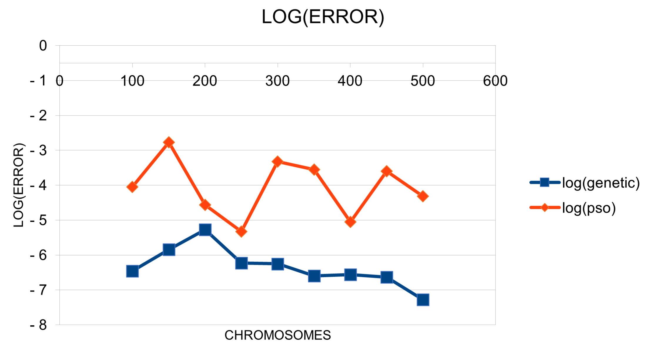
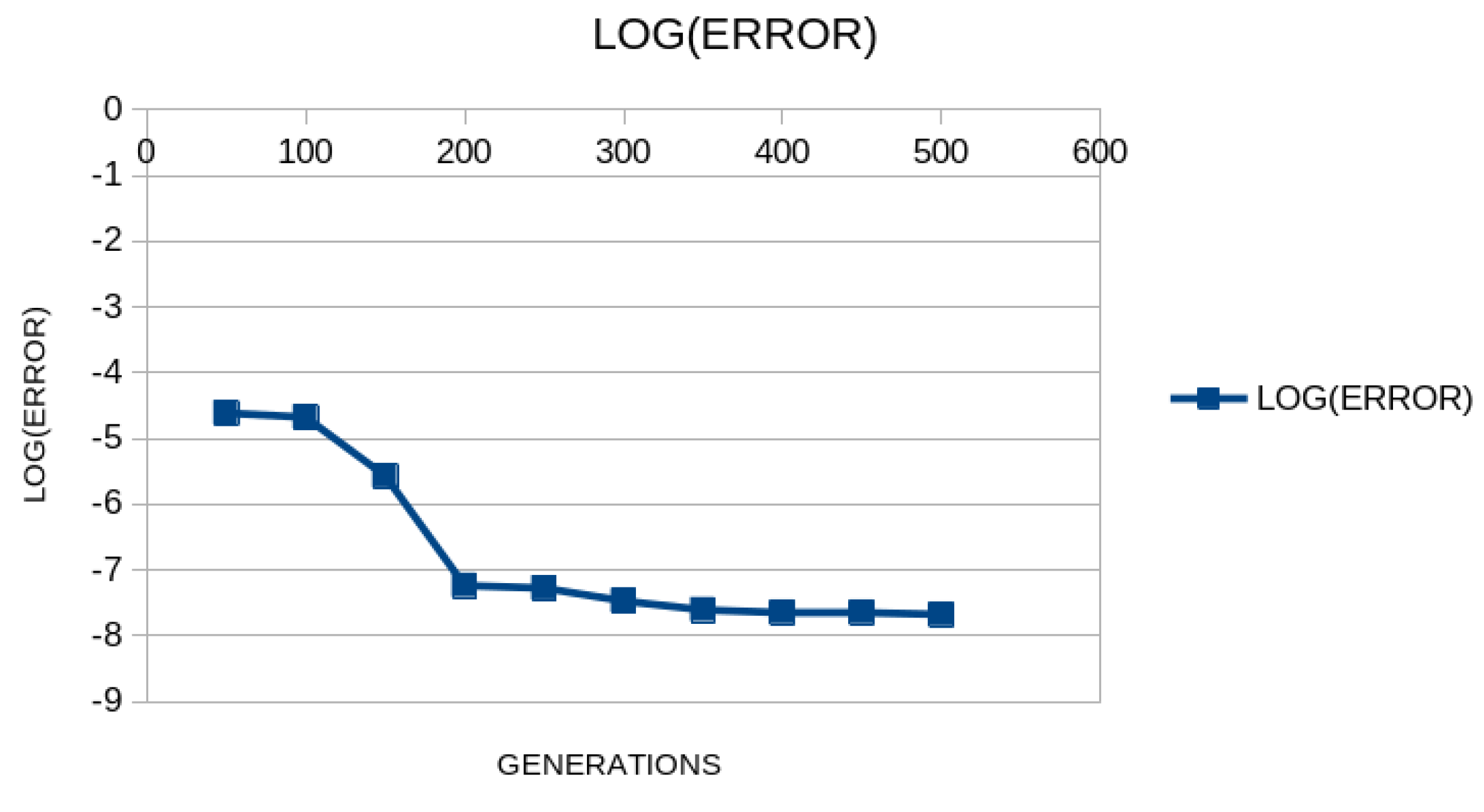
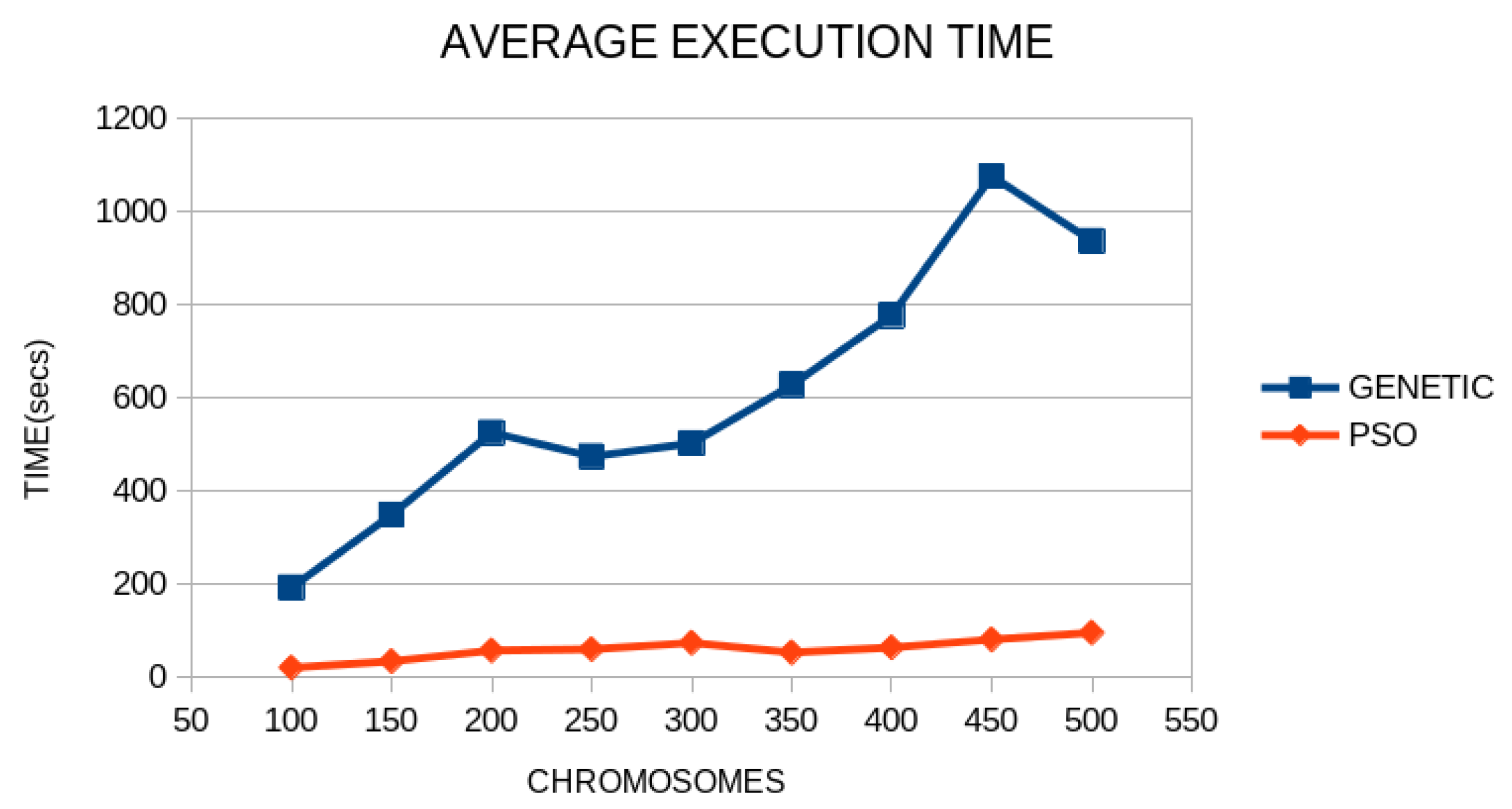
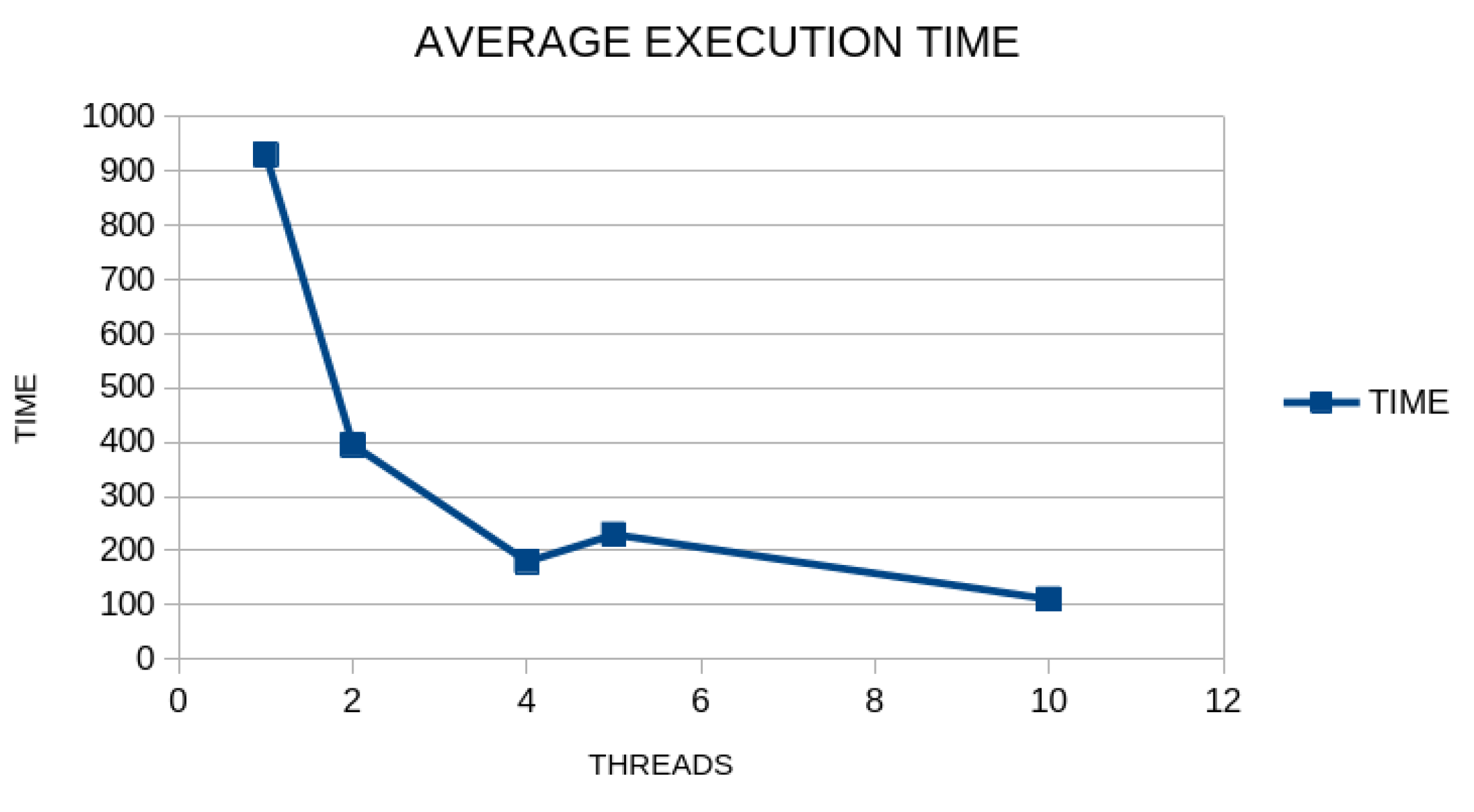
3. Results

The experiments were conducted using the freely available Optimus optimization environment, downloaded from https://github.com/itsoulos/GlobalOptimus/ (accessed on 7 December 2023). The execution machine was an AMD Ryzen 5950X with 128 GB of RAM, running Debian Linux, and the programs were compiled using the GNU C++ compiler. The values for the parameters of the used methods are shown in

Table 1. This table contains the values for the parameters used in the conducted experiments.

PARAMETER	MEANING	VALUE
d	Well width	5 nm
$t_0$	Left bound of Equation (14)	0.1
$t_1$	Right bound of Equation (14)	3.0
$NP$	Number of points used to divide the interval $[t_0,t_1]$	100
ℏ  ${\omega }_{L1}$	Longitudinal-optical phonon energy of material 1 (AlAs)	50.09 meV
ℏ  ${\omega }_{T1}$	Transverse-optical phonon energy of material 1 (AlAs)	44.88 meV
ℏ  ${\omega }_{L2}$	Longitudinal-optical phonon energy of material 2 (GaAs)	36.25 meV
ℏ  ${\omega }_{T2}$	Transverse-optical phonon energy of material 2 (GaAs)	33.29 meV
${ϵ}_{\infty ,1}$	High-frequency dielectric constant of material 1 (AlAs)	8.16
${ϵ}_{\infty ,2}$	High-frequency dielectric constant of material 2 (GaAs)	10.89
$N_C$	Number of chromosomes/particles	500
$N_G$	Maximum number of allowed generations	200
$p_S$	Selection rate	0.90
$p_M$	Mutation rate	0.05
$p_l$	Local search rate	0.01

. This table describes the simulation parameters for the objective problem as well as the parameters for the two global optimization techniques, previously described. The material parameters for semiconductors AlAs and GaAs, related to the frequencies and high-frequency dielectric constants, are taken from [3].

The dispersion curves of the interface phonon modes in a symmetric quantum well structure (GaAs/AlAs) are presented in Figure 1 and Figure 2. It is clear that the two branches correspond to the reststrahlen bands of the structure. It is obvious that the two different numerical algorithms (genetic and PSO algorithms) converge.

To evaluate the difference in execution time of the two techniques, an additional experiment was performed where the number of chromosomes/particles was varied from 100 to 500. The results of this experiment are illustrated graphically in Figure 3.

The PSO method significantly outperforms the genetic algorithm technique in execution time, and indeed, as the experimental results show, the genetic algorithm requires a significantly high execution time as the number of chromosomes increases. However, this problem can be smoothed over since genetic algorithms can by nature be parallelized relatively easily, as shown in a large number of related works [57,58,59]. Programming techniques that may be used to parallelize genetic algorithms are, for example, the MPI technique [60] or the OpenMP [61] programming library. For example, using the OpenMP library to parellelize the genetic algorithm, the graph of Figure 4 is obtained.

Furthermore, the logarithm of best values obtained by the two optimization methods for the equation is shown graphically in Figure 5.

From this graph, one can conclude that the genetic algorithm achieves significantly low values even for a limited number of chromosomes. In addition, the genetic algorithm, compared to the PSO technique, seems to maintain stability in its behavior regardless of the number of chromosomes used each time. Finally, the value of the objective function achieved using the genetic algorithm is significantly lower than the PSO technique.

Moreover, the logarithm for the best values obtained for Equation (13) for different number of maximum allowed generations is outlined in Figure 6. As can be seen from the graph, the error remains almost constant for more than 200 generations, which means that this number is enough to achieve the goal.

4. Discussion

In this paper, the IP modes in a heterostructure made with GaAs and AlAs were estimated using two different numerical methods (genetic algorithms and the PSO algorithm). The two branches denote the symmetric (S) and the antisymmetric (A) IP modes, as presented in Figure 1 and Figure 2. For small in-plane wavevectors, the difference between the symmetric and antisymmetric branches received the largest value, in contradiction to the case of large in-plane wavevectors, where the difference becomes small [3]. The IP modes are of crucial importance in estimating the electron/hole relaxation rates, dephasing rates, and decoherence processes in semiconductor quantum structures, among other quantum processes [2,3,4,5,6].

As can be seen from the conducted experiments, both the genetic algorithm technique and the particle swarm optimization technique manage to train the proposed model satisfactorily. However, after using a series of experiments with variation in the critical parameter of the number of chromosomes, it was found that the genetic algorithm requires significantly more computing time than the particle optimization technique, although it has more accuracy in the final result. This kind of problem can be alleviated by using parallel computing techniques since genetic algorithms by nature can be directly parallelized.

References

- Geng, H. Semiconductor Manufacturing Handbook, 1st ed.; McGraw-Hill Education: New York, NY, USA, 2005. [Google Scholar]
- Li, G.; Bleu, O.; Levinsen, J.; Parish, M.M. Theory of polariton-electron interactions in semiconductor microcavities. Phys. Rev. B 2021, 103, 195307. [Google Scholar] [CrossRef]
- Al-Dossary, O.; Babiker, M.; Constantinou, N.C. Fuchs-Kliewer interface polaritons and their interactions with electrons in GaAs/AlAs double heterostructures. Semicond. Sci. Technol. 1992, 7, 891–893. [Google Scholar] [CrossRef]
- Chu, H.; Chang, Y.-C. Phonon-polariton modes in superlattices: The effect of spatial dispersion. Phys. Rev. B 1988, 38, 12369. [Google Scholar] [CrossRef] [PubMed]
- Zhou, K.; Zhong, X.; Cheng, Q.; Wu, X. Actively tunable hybrid plasmon-phonon polariton modes in ferroelectric/graphene heterostructure systems at low-THz frequencies. Opt. Mater. 2022, 131, 112623. [Google Scholar] [CrossRef]
- Fuchs, R.; Kliewer, K.L. Oytical Modes of Vibration in an Ionic Crystal Slab. Phys. Rev. A 1965, 140, 2076. [Google Scholar] [CrossRef]
- Fuchs, R.; Kliewer, K.L. Optical Modes of Vibration in an Ionic Crystal Slab Including Retardation. II. Radiative Region. Phys. Rev. 1966, 150, 573. [Google Scholar]
- Rogalski, A. Infrared Detectors, 2nd ed.; CRC Press: Boca Raton, FL, USA, 2010. [Google Scholar]
- Kang, F.E.N.G.; Zhong-Ci, S.; Kang, F.; Zhong-Ci, S. Finite element methods. In Mathematical Theory of Elastic Structures; Springer: Berlin/Heidelberg, Germany, 1996; pp. 289–385. [Google Scholar]
- Stefanou, G. The stochastic finite element method: Past, present and future. Comput. Methods Appl. Mech. Eng. 2009, 198, 1031–1051. [Google Scholar] [CrossRef]
- Schenk, O.; Bollhöfer, M.; Römer, R.A. On large-scale diagonalization techniques for the Anderson model of localization. SIAM J. Sci. Comput. 2006, 28, 963–983. [Google Scholar] [CrossRef]
- Bishop, C. Neural Networks for Pattern Recognition; Oxford University Press: Oxford, UK, 1995. [Google Scholar]
- Cybenko, G. Approximation by superpositions of a sigmoidal Function. Math. Control. Signals Syst. 1989, 2, 303–314. [Google Scholar] [CrossRef]
- Baldi, P.; Cranmer, K.; Faucett, T.; Sadowski, P.; Whiteson, D. Parameterized neural networks for high-energy physics. Eur. Phys. J. C 2016, 76, 235. [Google Scholar] [CrossRef]
- Valdas, J.J.; Bonham-Carter, G. Time dependent neural network models for detecting changes of state in complex processes: Applications in earth sciences and astronomy. Neural Netw. 2006, 19, 196–207. [Google Scholar] [CrossRef] [PubMed]
- Carleo, G.; Troyer, M. Solving the quantum many-body problem with artificial neural networks. Science 2017, 355, 602–606. [Google Scholar] [CrossRef] [PubMed]
- Shirvany, Y.; Hayati, M.; Moradian, R. Multilayer perceptron neural networks with novel unsupervised training method for numerical solution of the partial differential equations. Appl. Soft Comput. 2009, 9, 20–29. [Google Scholar] [CrossRef]
- Malek, A.; Beidokhti, R.S. Numerical solution for high order differential equations using a hybrid neural network—Optimization method. Appl. Math. Comput. 2006, 183, 260–271. [Google Scholar] [CrossRef]
- Topuz, A. Predicting moisture content of agricultural products using artificial neural networks. Adv. Eng. Softw. 2010, 41, 464–470. [Google Scholar] [CrossRef]
- Escamilla-García, A.; Soto-Zarazúa, G.M.; Toledano-Ayala, M.; Rivas-Araiza, E.; Gastélum-Barrios, A. Applications of Artificial Neural Networks in Greenhouse Technology and Overview for Smart Agriculture Development. Appl. Sci. 2020, 10, 3835. [Google Scholar] [CrossRef]
- Shen, L.; Wu, J.; Yang, W. Multiscale Quantum Mechanics/Molecular Mechanics Simulations with Neural Networks. J. Chem. Theory Comput. 2016, 12, 4934–4946. [Google Scholar] [CrossRef]
- Manzhos, S.; Dawes, R.; Carrington, T. Neural network-based approaches for building high dimensional and quantum dynamics-friendly potential energy surfaces. Int. J. Quantum Chem. 2015, 115, 1012–1020. [Google Scholar] [CrossRef]
- Wei, J.N.; Duvenaud, D.; Aspuru-Guzik, A. Neural Networks for the Prediction of Organic Chemistry Reactions. ACS Cent. Sci. 2016, 2, 725–732. [Google Scholar] [CrossRef]
- Falat, L.; Pancikova, L. Quantitative Modelling in Economics with Advanced Artificial Neural Networks. Procedia Econ. Financ. 2015, 34, 194–201. [Google Scholar] [CrossRef]
- Namazi, M.; Shokrolahi, A.; Maharluie, M.S. Detecting and ranking cash flow risk factors via artificial neural networks technique. J. Bus. Res. 2016, 69, 1801–1806. [Google Scholar] [CrossRef]
- Tkacz, G. Neural network forecasting of Canadian GDP growth. Int. J. Forecast. 2001, 17, 57–69. [Google Scholar] [CrossRef]
- Baskin, I.I.; Winkler, D.; Tetko, I.V. A renaissance of neural networks in drug discovery. Expert Opin. Drug Discov. 2016, 11, 785–795. [Google Scholar] [CrossRef]
- Bartzatt, R. Prediction of Novel Anti-Ebola Virus Compounds Utilizing Artificial Neural Network (ANN). Chem. Fac. Publ. 2018, 49, 16–34. [Google Scholar]
- Tsoulos, I.; Gavrilis, D.; Glavas, E. Neural network construction and training using grammatical evolution. Neurocomputing 2008, 72, 269–277. [Google Scholar] [CrossRef]
- Rem, B.S.; Käming, N.; Tarnowski, M.; Asteria, L.; Fläschner, N.; Becker, C.; Sengstock, K.; Weitenberg, C. Identifying quantum phase transitions using artificial neural networks on experimental data. Nat. Phys. 2019, 15, 917–920. [Google Scholar] [CrossRef]
- Hermann, J.; Schätzle, Z.; Noé, F. Deep-neural-network solution of the electronic Schrödinger equation. Nat. Chem. 2020, 12, 891–897. [Google Scholar] [CrossRef]
- Cai, S.; Wang, Z.; Wang, S.; Perdikaris, P.; Karniadakis, G.E. Physics-Informed Neural Networks for Heat Transfer Problems. ASME. J. Heat Transf. 2021, 143, 060801. [Google Scholar] [CrossRef]
- Zhu, Q.; Liu, Z.; Yan, J. Machine learning for metal additive manufacturing: Predicting temperature and melt pool fluid dynamics using physics-informed neural networks. Comput. Mech. 2021, 67, 619–635. [Google Scholar] [CrossRef]
- Holland, J.H. Genetic algorithms. Sci. Am. 1992, 267, 66–73. [Google Scholar] [CrossRef]
- Stender, J. Parallel Genetic Algorithms: Theory & Applications; IOS Press: Amsterdam, The Netherlands, 1993. [Google Scholar]
- Doorly, D.J.; Peiró, J. Supervised Parallel Genetic Algorithms in Aerodynamic Optimisation. In Artificial Neural Nets and Genetic Algorithms; Springer: Vienna, Austria, 1997; pp. 229–233. [Google Scholar]
- Sarma, K.C.; Adeli, H. Bilevel Parallel Genetic Algorithms for Optimization of Large Steel Structures. Comput. Aided Civ. Infrastruct. Eng. 2001, 16, 295–304. [Google Scholar] [CrossRef]
- Fan, Y.; Jiang, T.; Evans, D.J. Volumetric segmentation of brain images using parallel genetic algorithms. IEEE Trans. Med. Imaging 2002, 21, 904–909. [Google Scholar]
- Leung, F.H.F.; Lam, H.K.; Ling, S.H.; Tam, P.K.S. Tuning of the structure and parameters of a neural network using an improved genetic algorithm. IEEE Trans. Neural Netw. 2003, 14, 79–88. [Google Scholar] [CrossRef] [PubMed]
- Sedki, A.; Ouazar, D.; El Mazoudi, E. Evolving neural network using real coded genetic algorithm for daily rainfall—Runoff forecasting. Expert Syst. Appl. 2009, 36, 4523–4527. [Google Scholar] [CrossRef]
- Majdi, A.; Beiki, M. Evolving neural network using a genetic algorithm for predicting the deformation modulus of rock masses. Int. J. Rock Mech. Min. Sci. 2010, 47, 246–253. [Google Scholar] [CrossRef]
- Kaelo, P.; Ali, M.M. Integrated crossover rules in real coded genetic algorithms. Eur. J. Oper. Res. 2007, 176, 60–76. [Google Scholar] [CrossRef]
- Tsoulos, I.G. Modifications of real code genetic algorithm for global optimization. Appl. Math. Comput. 2008, 203, 598–607. [Google Scholar] [CrossRef]
- Powell, M.J.D. A Tolerant Algorithm for Linearly Constrained Optimization Calculations. Math. Program. 1989, 45, 547–566. [Google Scholar] [CrossRef]
- Poli, R.; Kennedy, J.; Blackwell, T. Particle swarm optimization An Overview. Swarm Intell. 2007, 1, 33–57. [Google Scholar] [CrossRef]
- de Moura Meneses, A.A.; Machado, M.D.; Schirru, R. Particle Swarm Optimization applied to the nuclear reload problem of a Pressurized Water Reactor. Prog. Nucl. Energy 2009, 51, 319–326. [Google Scholar] [CrossRef]
- Shaw, R.; Srivastava, S. Particle swarm optimization: A new tool to invert geophysical data. Geophysics 2007, 72, F75–F83. [Google Scholar] [CrossRef]
- Ourique, C.O.; Biscaia Jr, E.C.; Pinto, J.C. The use of particle swarm optimization for dynamical analysis in chemical processes. Comput. Chem. Eng. 2002, 26, 1783–1793. [Google Scholar] [CrossRef]
- Fang, H.; Zhou, J.; Wang, Z.; Qiu, Z.; Sun, Y.; Lin, Y.; Chen, K.; Zhou, X.; Pan, M. Hybrid method integrating machine learning and particle swarm optimization for smart chemical process operations. Front. Chem. Sci. Eng. 2022, 16, 274–287. [Google Scholar] [CrossRef]
- Wachowiak, M.P.; Smolíková, R.; Zheng, Y.; Zurada, J.M.; Elmaghraby, A.S. An approach to multimodal biomedical image registration utilizing particle swarm optimization. IEEE Trans. Evol. Comput. 2004, 8, 289–301. [Google Scholar] [CrossRef]
- Marinakis, Y.; Marinaki, M.; Dounias, G. Particle swarm optimization for pap-smear diagnosis. Expert Syst. Appl. 2008, 35, 1645–1656. [Google Scholar] [CrossRef]
- Park, J.B.; Jeong, Y.W.; Shin, J.R.; Lee, K.Y. An Improved Particle Swarm Optimization for Nonconvex Economic Dispatch Problems. IEEE Trans. Power Syst. 2010, 25, 156–166. [Google Scholar] [CrossRef]
- Zhang, C.; Shao, H.; Li, Y. Particle swarm optimisation for evolving artificial neural network. In Proceedings of the IEEE International Conference on Systems, Man, and Cybernetics, Nashville, TN, USA, 8–11 October 2000; pp. 2487–2490. [Google Scholar]
- Yu, J.; Wang, S.; Xi, L. Evolving artificial neural networks using an improved PSO and DPSO. Neurocomputing 2008, 71, 1054–1060. [Google Scholar] [CrossRef]
- Charilogis, V.; Tsoulos, I.G. Toward an Ideal Particle Swarm Optimizer for Multidimensional Functions. Information 2022, 13, 217. [Google Scholar] [CrossRef]
- Eberhart, R.C.; Shi, Y.H. Tracking and optimizing dynamic systems with particle swarms. In Proceedings of the Congress on Evolutionary Computation, Seoul, Republic of Korea, 27–30 May 2001. [Google Scholar]
- Cantú-Paz, E.; Goldberg, D.E. Efficient parallel genetic algorithms: Theory and practice. Comput. Methods Appl. Mech. Eng. 2000, 186, 221–238. [Google Scholar] [CrossRef]
- Wang, K.; Shen, Z. A GPU-Based Parallel Genetic Algorithm for Generating Daily Activity Plans. IEEE Trans. Intell. Transp. Syst. 2012, 13, 1474–1480. [Google Scholar] [CrossRef]
- Kečo, D.; Subasi, A.; Kevric, J. Cloud computing-based parallel genetic algorithm for gene selection in cancer classification. Neural Comput. Appl. 2018, 30, 1601–1610. [Google Scholar] [CrossRef]
- Gropp, W.; Lusk, E.; Doss, N.; Skjellum, A. A high-performance, portable implementation of the MPI message passing interface standard. Parallel Comput. 1996, 22, 789–828. [Google Scholar] [CrossRef]
- Chandra, R.; Dagum, L.; Kohr, D.; Maydan, D.; McDonald, J.; Menon, R. Parallel Programming in OpenMP; Morgan Kaufmann Publishers Inc.: San Diego, CA, USA, 2001. [Google Scholar]