Dictionary Encoding Based on Tagged Sentential Decision Diagrams

Abstract

Encoding a dictionary into another representation means that all the words can be stored in the dictionary in a more efficient way. In this way, we can complete common operations in dictionaries, such as (1) searching for a word in the dictionary, (2) adding some words to the dictionary, and (3) removing some words from the dictionary, in a shorter time. Binary decision diagrams (BDDs) are one of the most famous representations of such encoding and are widely popular due to their excellent properties. Recently, some people have proposed encoding dictionaries into BDDs and some variants of BDDs and showed that it is feasible. Hence, we further investigate the topic of encoding dictionaries into decision diagrams. Tagged sentential decision diagrams (TSDDs), as one of these variants based on structured decomposition, exploit both the standard and zero-suppressed trimming rules. In this paper, we first introduce how to use Boolean functions to represent dictionary files and then design an algorithm that encodes dictionaries into TSDDs with the help of tries and a decoding algorithm that restores TSDDs to dictionaries. We utilize the help of tries in the encoding algorithm, which greatly accelerates the encoding process. Considering that TSDDs integrate two trimming rules, we believe that using TSDDs to represent dictionaries would be more effective, and the experiments also show this.

1. Introduction

A word is a string consisting of some symbols or characters, and a dictionary is a set that includes numerous words. A large dictionary can consist of millions of words. With the evolution of computer technology, in practical life, we use dictionaries in many places. For example, teachers store the names of all students in the school on their computers; this list of students is actually a dictionary, where each student’s name is a word. In order to solve practical problems, we often need to perform some common operations in dictionaries, three of which are, for example, (1) searching for a word in a dictionary, (2) adding words to a dictionary, and (3) removing words from a dictionary. In general, the time complexity of the above operations is $O\left(n\right)$. When the size of a dictionary (that is, the number of words) is too large, the above three operators are time-consuming and ineffective. Therefore, designing an effective method for operations in dictionaries is worth investigating.

An effective method for operations in dictionaries is to encode the dictionary into an efficient and compact representation. Some scholars have proposed a decision-diagram-based method of operation for dictionaries [1]. However, they have not provided any algorithms or implementations of the method. Following the above-mentioned idea, in this paper, we represent large dictionaries in decision diagrams and solve the common operations for dictionaries via operations in decision diagrams.

Binary decision diagrams (BDDs) are unique canonical forms that adhere to specific constraints, namely, ordering and reduction, ensuring that each Boolean function possesses a distinct BDD representation. This characteristic minimizes the storage requirements of BDDs and facilitates O(1) time equality tests on BDDs. After the emergence of the BDD, a variant known as the zero-suppressed BDD (ZDD) was introduced in [2]. ZDDs share similar characteristics with BDDs, such as canonicity and support for polynomial-time Boolean operations. The primary distinction between BDDs and ZBDDs lies in their respective reduction rules. Building on the applications of BDDs and ZBDDs, several extensions have been developed, including tagged BDDs (TBDDs) [3], chain-reduced BDDs (CBDDs) [1], chain-reduced ZDDs (CZDDs) [1], and edge-specified reduction BDDs (ESRBDDs) [4]. These extensions, which integrate two reduction rules, offer more compact representations compared to BDDs and ZDDs.

With the increasing maturity of decision diagram technology, people have begun to focus on research on applying decision diagrams to many fields. In ref. [1], the researchers successfully transformed a dictionary into BDDs and two variants of BDDs, CBDDs and CZDDs. They started from the following three points: (1) A Boolean function can be used to represent a binary number. (2) Decision diagrams can be used to represent Boolean functions. (3) Characters and symbols can be encoded into binary codes. Then, they considered the possibility of using decision diagrams to represent characters and symbols and implemented it. Finally, they encoded two dictionaries containing hundreds of thousands of words into three decision diagrams and provided data on the node count and time indicators. This confirms that encoding dictionaries into decision diagrams is a feasible research direction.

Hence, in this paper, we focus on applying another type of decision diagram, tagged sentential decision diagrams (TSDDs), into encoding dictionaries, and we first introduce TSDDs. To introduce TSDDs, we first introduce sentential decision diagrams (SDDs), which are decision diagrams based on structured decomposition [5], while BDDs are based on Shannon decomposition [6]. While BDDs are characterized by a total variable order, SDDs are defined by a variable tree (vtree), which is a complete binary tree with variables as its leaves, and apply standard trimming rules. Furthermore, in ref. [7], the researchers introduced the zero-suppressed variant of the SDD, known as the ZSDD, which also utilizes structured decomposition and applies zero-suppressed trimming rules instead of the standard trimming rules used in SDDs. ZSDDs offer a more compact representation for sparse Boolean functions compared to SDDs, while SDDs are better suited for homogeneous Boolean functions. To leverage the strengths of both SDDs and ZSDDs, ref. [8] devised a new decision diagram, the TSDD, which combines the standard and zero-suppressed trimming rules.

The contributions of our paper mainly include the following: (1) We propose an algorithm for encoding dictionaries into decision diagrams. We first transform a dictionary into a well-known data structure: the trie. With the help of tries, our algorithm can encode a dictionary into a decision diagram more efficiently than the method without tries. (2) We encoded 14 dictionaries into seven decision diagrams, i.e., BDDs, ZDDs, CBDDs, CZDDs, SDDs, ZSDDs, and TSDDs, in four ways, and we believe that TSDDs are the most suitable for representing dictionaries among all decision diagrams. We adopted TSDDs to represent dictionaries, and the experimental results show that TSDDs are more compact representations compared to other decision diagrams. (3) We also designed an algorithm that decodes a decision diagram and obtains the original dictionary. Our algorithm recursively restores each word in the dictionary and then saves these words together to obtain the original dictionary. Moreover, our algorithm can quickly complete the decoding process in most cases.

The rest of this paper is organized as follows. We first introduce the syntax and semantics of SDDs and ZSDDs. Section 3 introduces the syntax of TSDDs and the binary operation on TSDDs. In this section, we mainly introduce how to use a TSDD to denote a Boolean function and the trimming rules of TSDDs. Ref. [8] proposed a related definition of TSDDs. However, the researchers used three different semantics to explain SDDs, ZSDDs, and TSDDs. In fact, we believe that the difference in these decision diagrams mainly lies in the different trimming rules. These three decision diagrams can be explained with the same semantics. In this way, we can have a more intuitive understanding of these three decision diagrams and theoretically understand why TSDDs are more effective than SDDs and ZSDDs. Section 4 introduces how to use a Boolean function to represent a dictionary, the process of encoding a dictionary with the help of tries, and the decoding algorithm. An experimental evaluation comparing TSDDs with other decision diagrams appears in Section 5. Finally, Section 6 concludes this paper.

2. Preliminaries

Throughout this paper, we use lowercase letters (e.g., $x_1,x_2$) for variables and bold uppercase letters (e.g., $\mathbf{X},\mathbf{Y}$) for sets of variables. For a variable x, we use $\overline{x}$ to denote the negation of x. A literal is a variable or a negated one. A truth assignment over $\mathbf{X}$ is the mapping $\sigma :\mathbf{X}\mapsto \{0,1\}$. We let ${\Sigma }_{\mathbf{X}}$ be the set of truth assignments over $\mathbf{X}$. We say f is a Boolean function over $\mathbf{X}$, which is the mapping ${\Sigma }_{\mathbf{X}}\mapsto \{0,1\}$. We use $\mathbf{1}$ (resp. $\mathbf{0}$) for the Boolean function that maps all assignments to 1 (resp. 0).

Let $\mathbf{X}$ and $\mathbf{Y}$ be two disjoint and non-empty sets of variables. We use f to denote a Boolean function and use $f\left(\mathbf{X}\right)$ to denote a Boolean function over the variable set $\mathbf{X}$. We say the set $\{(f_1^p\left(\mathbf{X}\right),f_1^s\left(\mathbf{Y}\right)),\cdots ,(f_n^p\left(\mathbf{X}\right),f_n^s\left(\mathbf{Y}\right))\}$ is an $(\mathbf{X},\mathbf{Y})$-decomposition of a Boolean function $f(\mathbf{X},\mathbf{Y})$ iff $f=(f_1^p\left(\mathbf{X}\right)\wedge f_1^s\left(\mathbf{Y}\right))\vee \cdots \vee (f_n^p\left(\mathbf{X}\right)\wedge f_n^s\left(\mathbf{Y}\right))$, where every $f_i^p\left(\mathbf{X}\right)$ (resp. $f_i^s\left(\mathbf{Y}\right)$) is a Boolean function over $\mathbf{X}$ (resp. $\mathbf{Y}$). A decomposition is compressed iff $f_i^s\ne f_j^s$ for $i\ne j$. An $(\mathbf{X},\mathbf{Y})$-decomposition is called an $(\mathbf{X},\mathbf{Y})$-partition iff (1) $f_i^p\ne \mathbf{0}$ for $1\le i\le n$, (2) $f_i^p\wedge f_j^p=\mathbf{0}$ for $i\ne j$, and (3) $f_i^p\vee \cdots \vee f_n^p=\mathbf{1}$.

A vtree is a full binary tree whose leaves are labeled by variables, and we use $\mathbf{T}$ to denote a vtree node. Then, we use ${\mathbf{T}}_l$ to denote the left subtree of $\mathbf{T}$, while ${\mathbf{T}}_r$ denotes the right subtree of $\mathbf{T}$. The set of variables appearing in the leaves of $\mathbf{T}$ is denoted by $v\left(\mathbf{T}\right)$. In addition, there is a special leaf node labeled by 0, which can be considered a child of any vtree node, and $v\left(0\right)$ = ∅. The notation ${\mathbf{T}}^1\preccurlyeq {\mathbf{T}}^2$ denotes that ${\mathbf{T}}^1$ is a subtree of ${\mathbf{T}}^2$. In order to unify the definition, we use a tuple to denote a decision diagram in this paper and give the following definition.

Definition 1.

A decision diagram is a tuple $({\mathbf{T}}^1,{\mathbf{T}}^2,\alpha )$ s.t. ${\mathbf{T}}^2\preccurlyeq {\mathbf{T}}^1$, which is recursively defined as follows:

• α is a terminal node labeled by one of four symbols: $\mathbf{1}$, $\mathbf{0}$, ε, or $\overline{\epsilon }$;
• α is a decomposition node $\{(p_1,s_1),\cdots ,(p_n,s_n)\}$ satisfying the following:

  –

  Each $p_i$ is a decision diagram $({\mathbf{T}}^3,{\mathbf{T}}^4,\beta )$, where ${\mathbf{T}}^4\preccurlyeq {\mathbf{T}}^3\prec {\mathbf{T}}^2$;

  –

  Each $s_i$ is a decision diagram $({\mathbf{T}}^5,{\mathbf{T}}^6,\gamma )$, where ${\mathbf{T}}^6\preccurlyeq {\mathbf{T}}^5\prec {\mathbf{T}}^2$.

The size of $\alpha$ is denoted by $\left|\alpha \right|$, and $\left|\alpha \right|=0$ when $\alpha$ is a terminal node and $\left|\alpha \right|=n$ when $\alpha =\{(p_1,s_1),\cdots ,(p_n,s_n)\}$. We use $\langle ({\mathbf{T}}^1,{\mathbf{T}}^2,\alpha )\rangle$ to denote the Boolean function that this decision diagram represents. Then, we give the definition of the syntax of decision diagrams.

Definition 2.

Let ${\mathbf{T}}^1$ and ${\mathbf{T}}^2$ be two vtrees, and let ${\mathbf{T}}^2$ be a subtree of ${\mathbf{T}}^1$. The semantics of decision diagrams is inductively defined as follows:

• $\langle ({\mathbf{T}}^1,{\mathbf{T}}^2,\mathbf{1})\rangle ={\displaystyle \underset{x\in v\left({\mathbf{T}}^1\right)\setminus v\left({\mathbf{T}}^2\right)}{\bigwedge }}\overline{x}$, $\langle ({\mathbf{T}}^1,{\mathbf{T}}^2,\mathbf{0})\rangle =\mathbf{0}$.
• $\langle ({\mathbf{T}}^1,{\mathbf{T}}^2,\epsilon )\rangle ={\displaystyle \underset{v\left({\mathbf{T}}^1\right)}{\bigwedge }}\overline{x}$, $\langle ({\mathbf{T}}^1,{\mathbf{T}}^2,\overline{\epsilon })\rangle ={\displaystyle \underset{x\in v\left({\mathbf{T}}^1\right)\setminus v\left({\mathbf{T}}^2\right)}{\bigwedge }}\overline{x}\wedge {\displaystyle \underset{x\in v\left({\mathbf{T}}^2\right)}{\bigvee }}x$.
• $\langle ({\mathbf{T}}^1,{\mathbf{T}}^2,\{(p_1,s_1),\cdots ,(p_n,s_n)\})\rangle ={\displaystyle \underset{x\in v\left({\mathbf{T}}^1\right)\setminus v\left({\mathbf{T}}^2\right)}{\bigwedge }}\overline{x}\wedge {\displaystyle \underset{i=1}{\overset{n}{\bigvee }}}(\langle p_i\rangle \wedge \langle s_i\rangle )$ and satisfies the following conditions:

  –

  $\langle p_i\rangle \ne \mathbf{0}$ for $1\le i\le n$.

  –

  $\langle p_i\rangle \wedge \langle p_j\rangle$ for $i\ne j$.

  –

  ${\displaystyle \underset{i=1}{\overset{n}{\bigvee }}}\langle p_i\rangle =\mathbf{1}$.

A sentential decision diagram (SDD) $({\mathbf{T}}^1,{\mathbf{T}}^2,\alpha )$ has the following further constraints based on the above definition of a decision diagram:

• If $\alpha$ is a terminal node, then it must be one of the following:

  –

  $\langle (0,0,\mathbf{1})\rangle =\mathbf{1}$.

  –

  $\langle (0,0,\mathbf{0})\rangle =\mathbf{0}$.

  –

  $({\mathbf{T}}^1,0,\mathbf{1})$, where ${\mathbf{T}}^1$ must be a leaf vtree node.

  –

  $({\mathbf{T}}^1,{\mathbf{T}}^2,\overline{\epsilon })$, where ${\mathbf{T}}^1$ must be a leaf vtree node and ${\mathbf{T}}^1={\mathbf{T}}^2$.

• If $\alpha$ is a decomposable node, then ${\mathbf{T}}^1={\mathbf{T}}^2$.

Suppose that $({\mathbf{T}}^1,{\mathbf{T}}^2,\alpha )$ is an SDD; then, we know that ${\mathbf{T}}^1={\mathbf{T}}^2$ if $\alpha$ is a decomposable node. Hence, we use $(\mathbf{T},\mathbf{T},\alpha )$ to denote an SDD in order to provide a more intuitive definition of compression and trimming rules. The compression and trimming rules for SDDs are proposed in [9], and we give them according to the above definition.

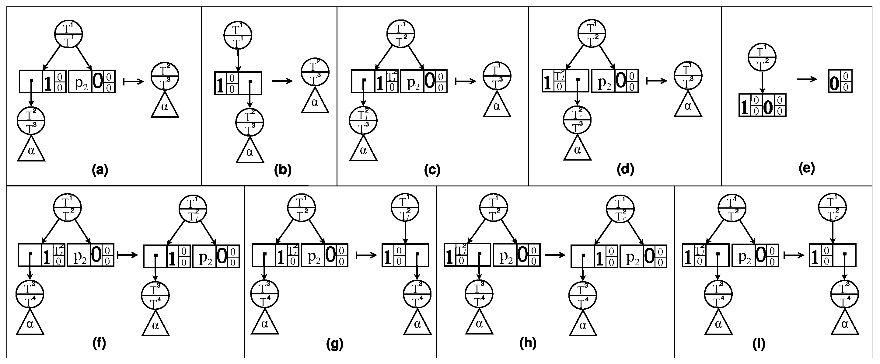
• Standard compression rule: if $\langle s_i\rangle =\langle s_j\rangle$, then replace $(\mathbf{T},\mathbf{T},\{(p_1,s_1),\cdots ,(p_i,s_i),\cdots ,(p_j,s_j),\cdots ,(p_n,s_n)\})$ with $(\mathbf{T},\mathbf{T},\{(p_1,s_1),\cdots ,(p^{\prime },s_i),\cdots ,(p_n,s_n)\})$, where $\langle p^{\prime }\rangle =\langle p_i\rangle \vee \langle p_j\rangle$.
• Standard trimming rules:

  –

  Replace $(\mathbf{T},\mathbf{T},\{(p_1,(0,0,\mathbf{1})),(p_2,(0,0,\mathbf{0}))\})$ with $p_1$ (shown in Figure 1a).

  –

  Replace $(\mathbf{T},\mathbf{T},\{(0,0,\mathbf{1}),s\left)\right\})$ with s (shown in Figure 1b).

For Figure 1, we need to clarify the following content. For a decision diagram $({\mathbf{T}}^1,{\mathbf{T}}^2,\alpha )$, when $\alpha$ is a terminal node, the above three components are represented by a square, where $\alpha$ is shown on the left side of the square, ${\mathbf{T}}^1$ is in the upper-right corner, and ${\mathbf{T}}^2$ is in the lower-right corner. When $\alpha$ is a decomposition node, ${\mathbf{T}}^1$ and ${\mathbf{T}}^2$ are displayed as circles with outgoing edges pointing to the elements. Each element $(p_i,s_i)$ is represented by paired boxes, where the left box represents the prime $p_i$, and the right box stands for the sub $s_i$.

Compressed and trimmed SDDs were shown to be a canonical form of Boolean functions in [9]. Then, we show the syntax and semantics of ZSDDs in our definition. A ZSDD has different constraints based on the above definition of a decision diagram. First of all, it should be noted that we use ${\mathbf{T}}_{root}$ to denote the root node of the whole vtree:

• If $\alpha$ is a terminal node, then it must be one of the following:

  –

  $\langle (\mathbf{T},0,\mathbf{1})\rangle ={\displaystyle \underset{v\left(\mathbf{T}\right)}{\bigwedge }}\overline{x}$.

  –

  $\langle (0,0,\mathbf{0})\rangle =\mathbf{0}$.

  –

  $({\mathbf{T}}_{root},\mathbf{T},\overline{\epsilon })$, where $\mathbf{T}$ must be a leaf vtree node.

  –

  $({\mathbf{T}}_{root},\mathbf{T},\mathbf{1})$, where $\mathbf{T}$ must be a leaf vtree node.

The compression and trimming rules for ZSDDs are as follows:

• Zero-suppressed compression rule: if $\langle s_i\rangle =\langle s_j\rangle$, then replace $({\mathbf{T}}^1,{\mathbf{T}}^2,\{(p_1,s_1),\cdots ,(p_i,s_i),\cdots ,(p_j,s_j),\cdots ,(p_n,s_n)\})$ with $({\mathbf{T}}^1,{\mathbf{T}}^2,\{(p_1,s_1),\cdots ,(p^{\prime },s_i),\cdots ,(p_n,s_n)\})$, where $\langle p^{\prime }\rangle =\langle p_i\rangle \vee \langle p_j\rangle$.
• Zero-suppressed trimming rules:

  –

  Replace $({\mathbf{T}}^1,{\mathbf{T}}^2,\{(({\mathbf{T}}_l^2,{\mathbf{T}}^3,\alpha ),({\mathbf{T}}_r^2,0,\mathbf{1})),(p_2,(0,0,\mathbf{0}))\})$ with $({\mathbf{T}}^1,{\mathbf{T}}^3,\alpha )$ (shown in Figure 1c).

  –

  Replace $({\mathbf{T}}^1,{\mathbf{T}}^2,\{({\mathbf{T}}_l^2,0,\mathbf{1}),({\mathbf{T}}_r^2,{\mathbf{T}}^3,\alpha )),(p_2,s_2)\})$ with $({\mathbf{T}}^1,{\mathbf{T}}^3,\alpha )$ (shown in Figure 1d).

Similar to SDDs, compressed and trimmed ZSDDs were also proven to be a canonical form of Boolean functions in [7]. SDDs are suitable to represent homogeneous Boolean functions, while ZSDDs are suitable to represent Boolean functions with sparse values.

3. Tagged Sentential Decision Diagrams

In this section, we will first introduce the syntax and semantics of TSDDs and the compression and trimming rules of TSDDs. Similar to SDDs and ZSDDs, we give the syntax and semantics based on the syntax and semantics of decision diagrams in Section 2. Then, we briefly introduce the binary operations on TSDDs and how to use these operations to construct a Boolean function.

3.1. Syntax and Semantics

TSDDs have different constraints compared to SDDs and ZSDDs based on the syntax and semantics of decision diagrams. Here, we give the following constraints.

Definition 3.

Let ${\mathbf{T}}^1$ and ${\mathbf{T}}^2$ be two vtrees s.t. ${\mathbf{T}}^2\preccurlyeq {\mathbf{T}}^1$ and $({\mathbf{T}}^1,{\mathbf{T}}^2,\alpha )$ is a TSDD. Then,

• If α is a terminal node, then it must be one of the following:

  –

  $(0,0,\mathbf{0})$, and $\langle (0,0,\mathbf{0})\rangle =\mathbf{0}$.

  –

  $({\mathbf{T}}^1,0,\mathbf{1})$, and $\langle ({\mathbf{T}}^1,0,\mathbf{1})\rangle ={\displaystyle \underset{v\left({\mathbf{T}}^1\right)}{\bigwedge }}\overline{x}$ (specifically, if ${\mathbf{T}}^1=0$, then $\langle (0,0,\mathbf{1})\rangle =\mathbf{1}$).

  –

  $({\mathbf{T}}^1,{\mathbf{T}}^2,\overline{\epsilon })$ and ${\mathbf{T}}^2$ must be a leaf vtree node, and $\langle ({\mathbf{T}}^1,{\mathbf{T}}^2,\overline{\epsilon })\rangle =({\displaystyle \underset{v({\mathbf{T}}^1)\setminus v({\mathbf{T}}^2)}{\bigwedge }}\overline{x})\wedge ({\displaystyle \underset{v({\mathbf{T}}^2)}{\bigvee }}x)$.

• If α is a decomposition node, then ${\mathbf{T}}^2$ must not be a leaf vtree node.

We can see that for a TSDD $({\mathbf{T}}^1,{\mathbf{T}}^2,\alpha )$, ${\mathbf{T}}^2$ must be a leaf vtree node or 0 if $\alpha$ is a terminal node. We should note that we can directly construct some TSDDs. (1) The TSDDs $(0,0,0)$ and $(0,0,1)$ can be constructed. (2) The TSDDs $(\mathbf{T},0,1)$ and $(\mathbf{T},\mathbf{T},\overline{\epsilon })$, where $\mathbf{T}$ is a leaf vtree node, can be constructed. These two kinds of TSDDs are special TSDDs; that is, they are the foundation for constructing a TSDD to represent a Boolean function. For the second type of TSDDs, we know that $\mathbf{T}$ is a leaf vtree node; that is, $v\left(\mathbf{T}\right)$ contains only one variable. Suppose that $v\left(\mathbf{T}\right)=x$; then, $\langle (\mathbf{T},0,1)\rangle =\overline{x}$ and $\langle \mathbf{T},\mathbf{T},\epsilon \rangle =x$.

3.2. Canonicity

TSDDs, as a variant of SDDs, apply trimming rules that integrate the trimming rules of SDDs and ZSDDs. Hence, the trimming rules of TSDDs include the trimming rules of SDDs and ZSDDs that are shown in Figure 1a–d, and we do not introduce them in the following definition. Hence, the trimming rules of TSDDs start from (e). In addition, these rules also include five new rules. We then show the compression and trimming rules for TSDDs as follows:

• Tagged compression rule: if $\langle s_i\rangle =\langle s_j\rangle$, then replace $({\mathbf{T}}^1,{\mathbf{T}}^2,\{(p_1,s_1),\cdots ,(p_i,s_i),\cdots ,(p_j,s_j),\cdots ,(p_n,s_n)\})$ with $({\mathbf{T}}^1,{\mathbf{T}}^2,\{(p_1,s_1),\cdots ,(p^{\prime },s_i),\cdots ,(p_n,s_n)\})$, where $\langle p^{\prime }\rangle =\langle p_i\rangle \vee \langle p_j\rangle$.
• Tagged trimming rules:

  –

  If $p=(0,0,\mathbf{1})$ and $s=(0,0,\mathbf{0})$, then replace $({\mathbf{T}}^1,{\mathbf{T}}^2,\left\{(p,s)\right\})$ with $(0,0,\mathbf{0})$ (shown in Figure 1e).

  –

  If $p_1=({\mathbf{T}}^3,{\mathbf{T}}^4,\alpha )$, $s_1=({\mathbf{T}}_r^2,0,\mathbf{1})$, $s_2=(0,0,\mathbf{0})$, and ${\mathbf{T}}_3\prec {\mathbf{T}}_l^2$, then replace $({\mathbf{T}}^1,{\mathbf{T}}^2,\{(p_1,s_1),$$(p_2,s_2)\left\}\right)$ with $({\mathbf{T}}^1,{\mathbf{T}}_l^2,\{(p_1,(0,0,\mathbf{1})),(p_2,(0,0,\mathbf{0}))\})$ (shown in Figure 1f).

  –

  If $p_1=({\mathbf{T}}^3,{\mathbf{T}}^4,\alpha )$, $s_1=({\mathbf{T}}_r^2,0,\mathbf{1})$, $s_2=(0,0,\mathbf{0})$, and ${\mathbf{T}}_3\prec {\mathbf{T}}_r^2$, then replace $({\mathbf{T}}^1,{\mathbf{T}}^2,\{(p_1,s_1),$$(p_2,s_2)\left\}\right)$ with $({\mathbf{T}}^1,{\mathbf{T}}_l^2,\left\{((0,0,\mathbf{1}),p_1)\right\})$ (shown in Figure 1g).

  –

  If $p_1=({\mathbf{T}}_l^2,0,\mathbf{1})$, $s_1=({\mathbf{T}}^3,{\mathbf{T}}^4,\alpha )$, $s_2=(0,0,\mathbf{0})$, and ${\mathbf{T}}_3\prec {\mathbf{T}}_l^2$, then replace $({\mathbf{T}}^1,{\mathbf{T}}^2,\{(p_1,s_1),$$(p_2,s_2)\left\}\right)$ with $({\mathbf{T}}^1,{\mathbf{T}}_r^2,\{(p_1,(0,0,\mathbf{1})),(p_2,(0,0,\mathbf{0}))\})$ (shown in Figure 1h).

  –

  If $p_1=({\mathbf{T}}_l^2,0,\mathbf{1})$, $s_1=({\mathbf{T}}^3,{\mathbf{T}}^4,\alpha )$, $s_2=(0,0,\mathbf{0})$, and ${\mathbf{T}}_3\prec {\mathbf{T}}_r^2$, then replace $({\mathbf{T}}^1,{\mathbf{T}}^2,\{(p_1,s_1),$$(p_2,s_2)\left\}\right)$ with $({\mathbf{T}}^1,{\mathbf{T}}_r^2,\left\{((0,0,\mathbf{1}),p_1)\right\})$ (shown in Figure 1i).

A TSDD is compressed (resp. trimmed) if no tagged compression (resp. trimming) rules can be applied to it. The canonicity of compressed and trimmed TSDDs was proved in [8].

3.3. Operations on TSDDs

The main operations on TSDDs include conjunction (∧), disjunction (∨), and negation ($\overline{x}$). The algorithm of the binary operations conjunction (∧) and disjunction (∨) was shown in [8]. Here, we show the negation algorithm on TSDDs in Algorithm 1.

Algorithm 1:  Negate $\left(F\right)$

   For special terminal nodes, which are the two kinds of TSDDs mentioned in Section 3.1, we can directly compute the resulting TSDD (Lines 1–2). For the other terminal nodes, we need to transform them into another form, namely, decomposable nodes (Line 3). And then, we apply $Negate\left(s_i\right)$ to every element and construct the following elements: $\gamma =\{(p_1,Negate\left(s_1\right)),\cdots ,(p_n,Negate\left(s_n\right))\}$; the resulting TSDD is $({\mathbf{T}}^1,{\mathbf{T}}^2,\gamma )$ (Lines 4–7). Finally, we apply compression and trimming rules to H (Line 8).

The binary operation is represented by $Apply(F,G,\circ )$, where ∘ represents ∧ or ∨, as shown in [8]. With these three operations, we can construct TSDDs to represent any Boolean function based on existing TSDDs. Here, we give an example. Given the Boolean function $f=\overline{(x_1\vee x_2)}\wedge (x_2\vee {\overline{x}}_3)$, we have the following initial TSDDs: $F\left(x_1\right)$, $F\left({\overline{x}}_1\right)$, $F\left(x_2\right)$, $F\left({\overline{x}}_2\right)$, $F\left(x_3\right)$, and $F\left({\overline{x}}_3\right)$, where $\langle F\left(x_1\right)\rangle =x_1$ and so on. The steps are as follows: (1) Let $F=Apply(F\left(x_1\right),F\left(x_2\right),\vee ))$. (2) Let $F=Negate\left(F\right)$. (3) Let $G=Apply(F\left(x_2\right),F\left({\overline{x}}_3\right),\vee )$. (4) Let $F=Apply(F,G,\wedge )$. Finally, we obtain TSDD F, where $\langle F\rangle =f$.

4. Encoding Dictionaries into TSDDs

A dictionary includes a large number of words, and we intend to transform it into a decision diagram that stores the whole dictionary. In this way, we can complete some common operations in the dictionary just by performing some binary operations on decision diagrams. When we want to verify whether a word exists in the dictionary, we just need to compute the result $Apply(F,G,\wedge )$, where F is the decision diagram representing the dictionary, and G is the decision diagram representing the word. If the result is $false$, then the word does not exist in the dictionary; otherwise, it exists in the dictionary. When we want to remove some words from the dictionary, we just need to construct the decision diagram G representing the set of words. And then, we compute the result $Apply(F,Negate(G),\wedge )$, where F represents the dictionary. Changing the traversal process on dictionaries to several binary operations on decision diagrams can remove the traversal process. This is why we encode dictionaries into decision diagrams.

In this section, we first introduce the process of encoding a dictionary into a decision diagram in four different ways. Ref. [1] pointed out the use of tries when encoding dictionaries into decision diagrams but did not provide a detailed description of the process. Hence, we were inspired by them and designed our method of encoding dictionaries with the help of tries, which greatly accelerated the compilation process. In the following, we intend to explain in detail how to use tries to complete the encoding of a dictionary and present the algorithm for decoding TSDDs.

4.1. Four Encoding Methods

The key to our method is to establish the correspondence between letters and numbers so that we can use a string of numbers to represent a word. For example, the ASCII code, a famous encoding system, uses a number ranging from 0 to 127 to represent 128 characters. With the help of the ASCII code, we represent a letter with some variables by transforming the code into its binary representation. As we know, the ASCII code of the letter ‘A’ is 65, whose binary representation is ‘1000001’ with 7 bits. We represent the letter ‘A’ by 7 variables, ‘$x_1{x}_2{x}_3{x}_4{x}_5{x}_6{x}_7$’, and consider the variable to be ‘0’ when the value is false and ‘1’ when the value is true. Hence, a letter needs 7 variables to be represented in the ASCII code. If a word consists of n letters, it needs 7*n variables in total to be represented.

However, there are many characters in the ASCII code that are often not used in most dictionaries, which means that it will cause significant redundancy if we use 7 bits to represent every letter. Suppose that a dictionary consists only of lowercase letters; that is, there are only 26 different letters in this dictionary. We number each letter in alphabetical order starting from 1, with the maximum number being 26, representing z. The number 26 just needs 5 bits to be represented, and its binary representation is ‘11010’, which means that a letter needs 5 variables to be represented. In this way, we reduce the number of variables required to represent a letter, and this code is called the compact code.

Compared with the ASCII code, the compact code can reduce the number of variables required to represent a letter. However, we need to make a protocol that specifies the correspondence between letters and numbers if we apply the compact code and records this correspondence in a table. This table is necessary for both encoding and decoding. Therefore, this table should be known as necessary information by all those who use compact encoding. The ASCCI code is an international standard that does not require additional space to store the correspondence between letters and codes. Hence, the universality of the ASCCI code is better than that of the compact code.

We use binary numbers to represent both the ASCII code and compact code for each letter, which means that the number of variables is the number of binary digits. Hence, we call this the binary way of encoding dictionaries. If the maximum value of the code is n, we can also use n variables to represent the code. For example, given the word zoo, there are two different letters, ‘z’ and ‘o’, in this word, and the word consists of three letters. Hence, we need six variables, $x_1,x_2,x_3,x_4,x_5$, and $x_6$, to represent it. $x_1$ and $x_2$ represent the first letter, and the first letter is ‘z’ if $x_1=true$ and $x_2=false$, while it is ‘o’ if $x_1=false$ and $x_2=true$. The other variables have similar meanings. Therefore, the word ‘zoo’ is represented by $x_1{x}_2{x}_3{x}_4{x}_5{x}_6=100101$. We call this the one-hot way of encoding the dictionary. A word consisting of m letters needs n*m variables in total to represent it in one-hot encoding, while it just needs $\lceil lo{g}_{2}n\rceil \ast m$ variables in total to represent it in a binary way.

4.2. Encoding with Tries

We can first encode every word in the dictionary into a TSDD one by one and then apply disjunction to these TSDDs to obtain the resulting TSDD that represents the whole dictionary. However, the process of encoding takes too much time, which is unacceptable to us. If the number of words in the dictionary exceeds 100,000, the encoding time will exceed two hours. Therefore, we first transform the dictionary into a trie, which is a multibranch tree, and then transform it into a TSDD. This can greatly accelerate the speed of encoding a dictionary.

A trie is a multibranch tree whose every node saves a letter, except for two special nodes. We know that a tree is a directed acyclic graph, and every node has its in- and out-degrees. In general, the in- and out-degrees of each node in a trie are both greater than 0, and these nodes all save a letter in them. However, there are two special nodes, one with an in-degree of 0 and the other with an out-degree of 0. We call the node with an in-degree of 0 the head and the node with an out-degree of 0 the tail. Both nodes do not save any letters. We can easily know that all paths in the trie must start from the head and end at the tail. A path represents a word in the dictionary, which means that the number of paths is the number of words in the trie.

We first introduce the algorithm for transforming a dictionary into a trie in Algorithm 2. We need to initialize the two special nodes, that is, the head node $\tilde{h}$ and the tail node $\tilde{t}$, and a node $\tilde{v}$, which is an empty node (Line 1). Then, we traverse each word in the dictionary, and in a loop, we let $\tilde{v}$ be the node $\tilde{h}$ (Lines 2–3). We perform the following operations on the letters in the word in order. The operation $Find(l,\tilde{v})$ means we look for a node from successor nodes of $\tilde{v}$ that save the letter l. If such a node does not exist, we create a new node with NewNode(l) and let it be the successor node of trace with $Append(\tilde{v},\tilde{n})$ (Lines 4–8), and then we let $\tilde{v}$ be the node $\tilde{n}$ (Line 9). After all the letters have been accessed, we let $\tilde{t}$ be the successor node of $\tilde{v}$ (Line 10). Finally, the node $\tilde{h}$ is the resulting trie.

Algorithm 2:  ToTrie $\left(D\right)$

After we obtain the trie, we need to compress it further. Firstly, the nodes in the trie need to be assigned an important parameter: depth; we denote a node as $\tilde{P}(d,l)$, where d stands for depth and l stands for letter. We first give the following definition.

Definition 4.

A trie node $\tilde{P}(d,l)$ is defined as follows:

• $d=0$ if the node $\tilde{P}(l,d)$ is the node $head$.
• If $\tilde{P}(d,l)$ is a node and ${\tilde{P}}^{\prime }(d^{\prime },l^{\prime })$ is one of its children, then $d^{\prime }=d+1$.
• Letters that appear sequentially in the path from the root to the leaf form a word.

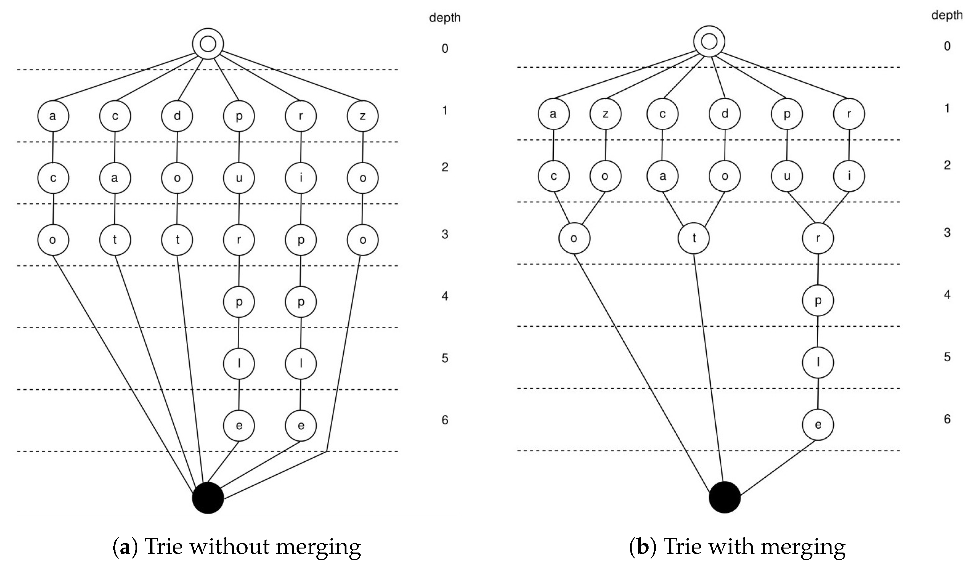
The step of compressing the trie entails merging two nodes that have the same depth and meet certain conditions into one node. The conditions are as follows: (1) The two nodes save the same letter. (2) The two nodes have the same children nodes. We group all nodes by depth and merge nodes by group, starting from the deepest group.

Here, we give an example using a dictionary that contains six words: aco, cat, dot, purple, ripple, and zoo. The tries before and after merging the nodes are shown in Figure 2. There are two special nodes in the graph, namely, the root node with a depth of 0 and the tail node represented by a solid circle without a depth. Except for these two nodes, each other node stores a letter, and we stipulate that all paths representing words start at the root node and end at the tail node. Except for the tail node, all other nodes have a depth, and the maximum depth on a path is the number of letters in the word represented by that path. After we merge the nodes, we can see that the number of nodes has significantly decreased.

We then transform this trie into a TSDD, and the algorithm is shown in Algorithm 3. We first compute the number of variables in the TSDD and suppose that the maximum length of all words in the dictionary is n and the number of different letters in the dictionary is m. The number of variables is 128*n if we use the ASCII code in a one-hot way and 7*n if we use the ASCII code in a binary way. The number of variables is m*n if we use the compact code in a one-hot way and $\lceil lo{g}_{2}m\rceil \ast n$ if we use the compact code in a binary way. Here, we explain the method that transforms a trie node into a TSDD node by using the ASCII code in a binary way, and we save the corresponding TSDD in the trie node. There are three steps in total. Let $\tilde{P}$ be a trie node. The steps are as follows: (1) We access each node $\tilde{n}(d,l)$ from bottom to top and compute the result of applying disjoin on all the TSDDs that are saved in the successor nodes of $\tilde{n}(d,l)$ and record this result as G, and Successor($\tilde{n}$) represents all the successor nodes of the trie node $\tilde{n}$ (Lines 1–4). (2) We compute the TSDD GetTSDD($\tilde{n}$), which represents the letter saved in the trie node (Line 5). For example, if the letter l is ‘a’, the binary representation of the letter is ‘1100001’, and the related variables are $x_{(d-1)\ast 7+1},x_{(d-1)\ast 7+2},x_{(d-1)\ast 7+3},x_{(d-1)\ast 7+4},x_{(d-1)\ast 7+5},x_{(d-1)\ast 7+6},x_{(d-1)\ast 7+7}$. Of these variables, the variables that are marked as ‘1’ are $x_{(d-1)\ast 8+1},x_{(d-1)\ast 8+2},x_{(d-1)\ast 8+7}$. We need to construct the TSDD G that represents the Boolean function $f=x_{(d-1)\ast 7+1}\wedge x_{(d-1)\ast 7+2}\wedge {\overline{x}}_{(d-1)\ast 7+3)}\wedge {\overline{x}}_{(d-1)\ast 7+4}\wedge {\overline{x}}_{(d-1)\ast 7+5}\wedge {\overline{x}}_{(d-1)\ast 7+6}\wedge x_{(d-1)\ast 7+7}$. (3) We compute the TSDD $G=Apply(G,GetTSDD\left(\tilde{n}\right),\wedge )$ (Line 5). Then, we save this TSDD G in the trie node (Line 6). Similarly, we group all trie nodes based on depth and transform the nodes into TSDDs in the group in descending order of depth. We should note that if $\tilde{P}$ is the tail trie node, the TSDD saved in it is not fixed. The TSDD saved in the tail trie node is decided based on the depth of its parent node. Let the depth of the parent node be d and the TSDD saved in the tail node be G; then, $\langle G\rangle ={\displaystyle \underset{i=d\ast 7+1}{\overset{n}{\bigwedge }}}\overline{x}$. In addition, not all words consist of n letters. If a word consists of fewer than n letters, we use null characters to supplement the remaining positions. For the above example, if the letter saved in the trie node is a null character, then the Boolean function in step 2 is $f={\overline{x}}_{(d-1)\ast 7+1}\wedge {\overline{x}}_{(d-1)\ast 7+2}\wedge {\overline{x}}_{(d-1)\ast 7+3}\wedge {\overline{x}}_{(d-1)\ast 7+4)}\wedge {\overline{x}}_{(d-1)\ast 7+5}\wedge {\overline{x}}_{(d-1)\ast 7+6}\wedge {\overline{x}}_{(d-1)\ast 7+7}$. Finally, the TSDD saved in the head trie node is the TSDD that represents the whole dictionary (Line 7).

Algorithm 3:  ToTSDD $\left(\tilde{P}\right)$

For the other three encoding methods, the process is also similar, with only differences in the relevant variables. Similarly, it is necessary to perform a conjunction operation on the variables marked as 1 and the negation of variables marked as 0. The TSDD saved in the head trie node is what we want. At this point, the process of encoding a dictionary is complete.

4.3. Decoding

We use one code to represent a letter and then multiple codes to represent an entire word. On the contrary, we can also restore a word from a code string. The process of decoding a TSDD means restoring a string of code from the TSDD and then obtaining the corresponding words. After restoring all strings of codes, we can obtain the original dictionary.

Before explaining the decoding algorithm, we first introduce some operations. Given a depth d, we use List(d) to denote the set of all possible TSDDs, that is, the TSDDs representing the possible letters. In Section 4.1, we gave an example of how to represent the word zoo with six variables by using the compact code in a binary way. Now, we continue to use this example to illustrate the decoding process. In addition, the variables denote a null character when both $x_1$ and $x_2$ are assigned the value ’false’. Hence, there are three cases when the depth is 1. $List\left(1\right)=\{F_1,F_2,F_3\}$, where $F_1$, $F_2$, and $F_3$ are TSDDs, and $\langle F_1\rangle ={\overline{x}}_1\wedge {\overline{x}}_2$, $\langle F_2\rangle ={\overline{x}}_1\wedge x_2$, and $\langle F_3\rangle =x_1\wedge {\overline{x}}_2$. We also use Letter(F) to denote the letter that the TSDD F represents; that is, $Letter\left(F_1\right)$ is a null character, $Letter\left(F_2\right)=$‘z’, and $Letter\left(F_3\right)=$ ‘o’. Given the word ‘zo’, we stipulate that Push(‘zo’,‘o’) = ‘zoo’ and $Pop$(‘zoo’) = ‘zo’. We use $d_{max}$ to denote the max depth in the dictionary. The algorithm is shown in Algorithm 4.

The initial inputs for this algorithm are the TSDD to be decoded, the empty word w, the empty dictionary $\overline{D}$, and the depth d = 1. Then, we make the operation $Apply(F,G,\wedge )$, where G represents the letter that may appear in the word in order (Lines 1–2). If the result of $Apply(F,G,\wedge )$ is not false, we recursively add the next possible letter until we encounter a null character or reach the maximum depth (Lines 3–10). After the algorithm is completed, the dictionary $\overline{D}$ is the result we want.

However, this algorithm is suitable for decision diagrams with fewer variables. We can decode decision diagrams that are encoded in a binary way but not decision diagrams that are encoded in a one-hot way. This is because the time for decoding a decision diagram that is encoded in a one-hot way exceeds one hour when the dictionary includes over 10,000 words. Hence, we need another effective algorithm to decode such decision diagrams. In this study, we did not conduct decoding-related experiments.

Algorithm 4:  Decode $(F,w,\overline{D},d)$

5. Experimental Results

In this section, we first compare the speed of encoding a dictionary with and without tries to demonstrate the acceleration effect of tries on encoding a dictionary. We then encode 14 dictionaries into BDDs, ZDDs, CBDDs, CZDDs, SDDs, ZSDDs, and TSDDs with tries and compare the node count of decision diagrams and the time required for encoding the dictionaries into decision diagrams. All experiments were carried out on a machine equipped with an Intel Core i7-8086K 4 GHz CPU and 64 GB RAM. We used four encoding methods to conduct all experiments: compact code in a one-hot way, compact code in a binary way, ASCII code in a one-hot way, and ASCII code in a binary way.

The dictionaries we used are the English words in the file /usr/shar/dict/words on a MacOS system with 235,886 words with a length of up to 24 from 54 symbols, a password list with 979,247 words with a length of up to 32 from 79 symbols [10], and other word lists from the website at [11]. To compare the time for encoding dictionaries into TSDDs with and without tries, we separated the first 20,000, 30,000, and 40,000 words from the dictionary words to form four new dictionaries and encoded them into TSDDs. This is because, without the help of a trie, the encoding time would exceed two hours when the number of words exceeds 40,000. We used the same right linear vtree to complete the first experiment. Hence, the size and node count of TSDDs must be the same in this experiment with the same encoding method, and we only compared the encoding time. The results are shown in

Table 1. The time (secs.) for encoding dictionaries with and without tries.

Word Count		Compact, One-Hot	Compact, Binary	ASCII, One-Hot	ASCII, Binary
20,000	with trie	3.527	2.228	4.23	3.119
	without trie	251.86	412.156	292.52	842.622
30,000	with trie	5.509	3.326	5.084	3.702
	without trie	650.39	994.768	677.524	1511.209
40,000	with trie	7.141	3.927	7.677	5.503
	without trie	1125.327	1682.585	1100.168	2500.582

.

We can see that all the experiments were completed within 10 s with the help of tries for these three dictionaries. When we did not rely on the help of tries, even the minimum encoding time reached 251.86 s (the compact code in a one-hot way for the dictionary with 20,000 words). When the number of words reaches 40,000, it even takes over 1000 s to encode the dictionary, which exceeds the time required for encoding the dictionary with the help of tries by more than a hundred times. It can be inferred that for dictionaries with more words, encoding them will take more time, which we cannot tolerate. Therefore, we can see that tries have excellent acceleration effects when we encode a dictionary, and it is necessary to rely on the help of tries when encoding dictionaries.

Then, the second experiment is as follows. Ref. [1] encoded two dictionaries, words and password, into four decision diagrams, i.e., BDDs, ZDDs, CBDDs, and CZDDs, in four ways and gave the number of nodes of decision diagrams and the encoding times for some data. Here, we use their data and record them in

Table 2. The comparison of SDDs, ZSDDs, and TSDDs over 2 categories of benchmarks.

Dictionary	Word Count	Decision Diagram	Compact, One-Hot		Compact, Binary		ASCII, One-Hot		ASCII, Binary
			Node Count	Time/s	Node Count	Time/s	Node Count	Time/s	Node Count	Time/s
words	235,886	BDD	9,701,439	770.114	1,117,454	102.74	23,161,501	2583.639	1,464,773	116.729
		ZDD	297,681	48.78	723,542	13.11	297,681	173.56	851,580	14.4
		CBDD	626,070	97.671	1,007,868	69.721	626,071	96.365	1,277,640	117.756
		CZDD	297,681	15.04	723,542	9.7	297,681	21.84	851,580	10.2
		SDD	9,560,113	745.614	300,235	235.774	23,106,545	2011.952	536,433	260.563
		ZSDD	298,995	221.506	443,883	224.212	305,323	225.827	740,462	248.558
		TSDD	358,778	233.301	215,588	109.899	360,797	228.642	191,762	209.041
password	979,247	BDD	49,231,085	3513.906	4,422,292	1061.895	79,014,931	3582.56	4,943,940	963.165
		ZDD	1,130,729	713.15	2,506,088	52.52	1,130,729	658.21	2,875,612	50.77
		CBDD	2,321,572	1734.869	3,597,474	710.504	2,321,792	1466.674	4,307,614	1466.614
		CZDD	1,130,729	46.73	2,506,088	30.62	1,130,729	57.81	2,875,612	30.33
		SDD	-	-	3,648,973	1074.062	-	-	3,979,717	1,348.212
		ZSDD	1,146,448	432.112	1,744,536	562.329	1,188,576	440.762	2,866,480	919.113
		TSDD	1,356,869	1316.681	1,101,669	510.276	1,366,130	927.079	2,426,472	792.076
Ashley- Madison	375,853	BDD	–	–	2,111,727	364.746	–	–	2,082,848	280.353
		ZDD	548,365	103.033	922,478	154.342	547,753	112.371	1,326,746	220.22
		CBDD	548,724	498.307	1,033,895	199.4	695,493	427.79	1,435,585	3301.287
		CZDD	548,365	83.179	922,475	131.328	547,753	102.695	1,326,745	200.374
		SDD	-	-	1,671,665	525.145	-	-	1,656,556	518.945
		ZSDD	560,898	273.59	923,129	273.59	564,650	297.303	1,280,338	423.104
		TSDD	596,396	351.467	420,810	228.901	595,493	369.138	965,362	333.126
cain-and -abel	306,706	BDD	10,056,981	887.681	1,158,528	100.348	23,800,813	2660.446	1,298,518	116.788
		ZDD	317,745	35.482	623,053	68.525	317,519	43.817	873,020	93.901
		CBDD	318,014	102.549	623,083	84.873	317,768	99.385	872,924	122.171
		CZDD	317,675	32.672	623,033	58.034	317,394	38.553	872,958	80.506
		SDD	9,919,042	1006.302	494,076	286.032	23,665,165	2860.691	693,425	312.641
		ZSDD	319,387	235.417	623,169	274.117	323,398	227.594	789,973	289.935
		TSDD	382,102	253.088	233,681	219.508	383,978	271.741	221,983	225.274
dutch _wordlist	679,006	BDD	–	–	1,532,202	283.513	–	–	1,497,917	270.681
		ZDD	434,264	111.298	730,174	159.714	416,140	119.327	977,282	221.458
		CBDD	434,853	649.243	730,142	236.863	416,667	520.259	976,921	332.901
		CZDD	434,264	100.395	730,103	131.916	416,140	102.627	977,208	205.869
		SDD	-	-	1,113,678	484.359	-	-	1,124,797	469.573
		ZSDD	462,359	275.034	665,840	322.585	449,766	271.683	977,282	432.675
		TSDD	521,416	648.479	315,129	276.333	504,568	603.326	273,022	310.324
honeynet2	226,928	BDD	16,684,568	1805.869	1,153,693	123.618	20,820,911	2822.858	1,135,440	121.942
		ZDD	290,592	45.767	507,574	62.566	287,032	44.778	737,354	103.399
		CBDD	290,974	181.046	507,561	81.879	287,392	136.038	737,267	121.531
		CZDD	290,542	40.384	507,515	54.568	286,975	37.238	737,280	99.295
		SDD	16,498,545	2618.111	365,332	541.942	-	-	338,896	509.53
		ZSDD	306,700	425.001	492,636	496.043	306,572	426.833	738,166	523.851
		TSDD	375,037	563.074	224,538	284.982	376,022	557.861	193,971	407.62
honeynet	226,081	BDD	16,678,501	1832.591	1,154,555	132.447	20,820,787	2878.694	1,135,434	124.669
		ZDD	289,337	56.012	481,969	69.611	287,033	44.508	737,354	105.59
		CBDD	289,719	185.336	481,947	78.524	287,392	132.029	737,267	123.408
		CZDD	289,337	47.135	481,888	60.258	287,033	40.667	737,280	100.879
		SDD	-	-	332,475	516.381	-	-	336,096	521.902
		ZSDD	302,318	424.39	481,176	475.143	304,772	424.651	672,556	492.475
		TSDD	374,666	955.063	200,047	322.606	373,872	710.177	207,326	430.065
honeynet- withcount	226,928	BDD	19,411,188	1912.06	1,340,803	130.746	24,073,981	2877.532	1,314,007	129.876
		ZDD	323,725	50.566	584,377	63.843	320,206	54.416	847,306	124.843
		CBDD	324,089	173.293	584,351	86.678	320,558	141.628	847,198	128.246
		CZDD	323,725	46.186	584,317	58.419	320,206	47.772	847,220	107.445
		SDD	19,037,012	2176.356	383,858	562.195	-	-	438,056	555.949
		ZSDD	338,609	436.965	585,246	475.067	340,241	432.563	822,046	530.876
		TSDD	416,101	438.361	214,368	405.273	417,684	426.115	214,044	425.736
mssql- passwords	172,696	BDD	6,033,921	538.622	445,940	24.096	7,852,025	827.749	430,156	23.884
		ZDD	96,032	6.446	217,338	14.304	95,379	7.727	266,125	18.321
		CBDD	96,393	40.944	217,329	18.009	95,743	33.264	266,086	23.042
		CZDD	96,038	6.468	217,332	13.276	95,385	7.668	266,106	17.458
		SDD	5,996,363	733.865	86,651	103.127	7,843,567	917.801	86,137	118.743
		ZSDD	110,101	392.158	133,880	325.367	118,332	436.18	673,709	876.657
		TSDD	124,794	222.714	85,109	44.981	127,391	237.564	80,504	52.27
phpbb- cleaned-up	184,364	BDD	19,685,391	2767.214	1,473,949	176.6	–	–	1,466,049	178.394
		ZDD	344,154	58.099	646,617	84.216	344,382	50.182	905,808	125.349
		CBDD	344,488	247.555	626,625	116.836	344,681	210.924	905,717	162.292
		CZDD	344,154	53.096	626,588	83.761	344,382	49.099	905,750	120.685
		SDD	19,570,745	2092.278	773,398	380.189	-	-	790,332	374.249
		ZSDD	352,559	233.575	626,852	281.159	358,112	232.441	905,946	320.189
		TSDD	446,421	447.709	277,164	220.467	444,665	394.971	231,022	261.902
phpbb	184,388	BDD	19,915,225	2623.845	1,475,978	186.136	–	–	1,467,977	169.521
		ZDD	344,468	56.859	627,422	72.915	344,680	56.34	906,562	120.612
		CBDD	344,800	226.646	627,429	95.844	344,976	190.775	906,471	138.621
		CZDD	344,468	54.703	627,393	88.244	344,680	55.07	906,504	120.922
		SDD	19,637,384	2196.641	775,524	376.349	-	-	791,935	375.543
		ZSDD	353,976	239.4	627,657	281.859	358,506	273.315	906,699	312.853
		TSDD	445,432	369.997	278,763	255.027	448,969	418.608	236,446	241.572
phpbb- withcount	184,389	BDD	21,291,701	2903.687	1,584,038	205.257	–	–	1,573,792	202.202
		ZDD	365,847	70.259	695,364	99.788	365,573	84.197	972,290	147.415
		CBDD	366,120	260.719	695,356	137.425	365,835	234.62	972,220	194.979
		CZDD	365,847	72.25	695,303	106.178	365,573	79.704	972,236	133.168
		SDD	-	-	800,791	387.881	-	-	774,597	355.65
		ZSDD	374,969	240.648	692,190	277.569	379,074	239.707	972,429	318.899
		TSDD	473,851	355.424	302,141	195.59	477,819	366.837	481,863	301.143
walk- the-line	279,616	BDD	22,526	1.716	3882	0.19	90,111	14.994	4730	0.223
		ZDD	880	0.042	1764	0.019	880	0.136	2415	0.081
		CBDD	892	0.101	1794	0.03	892	0.266	2439	0.099
		CZDD	892	0.059	1794	0.046	892	0.127	2439	0.078
		SDD	5980	30.196	1384	0.659	71,458	195.537	1913	1.066
		ZSDD	2016	1.093	1198	0.165	5202	2.099	1421	0.25
		TSDD	1627	1.912	1175	0.33	4187	6.281	1269	1.634
xato-net- 10-million	755,995	BDD	–	–	3,055,697	760.534	–	–	3,022,307	659.394
		ZDD	853,731	499.188	1,372,273	270.62	850,452	198.032	1,944,759	396.952
		CBDD	854,287	1364.918	1,372,115	467.862	850,973	1130.453	1,944,325	678.649
		CZDD	853,731	492.349	1,372,123	262.815	850,452	236.005	1,944,387	664.089
		SDD	-	-	2,409,752	1056.438	-	-	2,313,320	1,074.787
		ZSDD	859,361	538.169	1,358,287	662.663	860,536	570.875	1,877,647	793.756
		TSDD	1,055,763	1537.339	665,174	629.051	1,052,745	1745.605	1,279,015	776.298

. For the other 12 dictionaries, they did not conduct any relevant experiments. Therefore, we extended their experiment by encoding the remaining twelve dictionaries into BDDs, ZDDs, CBDDs, and CZDDs in four ways and recording the node count and encoding time. We also encoded the 14 dictionaries into SDDs, ZSDDs, and TSDDs in four ways and then compared all decision diagrams using two categories of benchmarks: node count, the node count of decision diagrams, and time, the time for encoding a dictionary. The initial vtrees are all right linear trees. To reduce the node count of decision diagrams, we designed minimization algorithms for ZSDDs and TSDDs and applied them once to SDDs, ZSDDs, and TSDDs when over half of the words in the dictionary were encoded. The results of this experiment are shown in Table 2. Columns 1–2 report the names of the dictionaries and the word counts of the dictionaries. The names of the decision diagrams that represent the dictionaries are reported in column 3. Then, columns 4–11 report the node counts of decision diagrams and the encoding times using the four encoding methods. In our experiment, each dictionary contained over 100,000 words. In addition, we use ’–’ in place of data if the encoding time exceeded one hour.

In general, the number of variables used in one-hot encoding is much larger than that in binary encoding, and the Boolean functions encoded in a one-hot way are more sparse than those encoded in a binary way when representing the same dictionary. For each dictionary, the node count of the decision diagram with the minimum node count among all decision diagrams for each encoding method is highlighted in bold so that readers can intuitively see which decision diagram performs the best in node count. We first consider the decision diagrams that are encoded with the compact code in a one-hot way. Taking the dictionary phpbb as an example, we can see that the ZDD and CZDD have the same and minimum node counts, while the CBDD has the second-smallest node count among all decision diagrams. The node count of the CBDD is 344,800, which is just 332 more than that of the BDD and CZDD. The node count of the ZSDD is larger than that of the ZDD, CZDD, and CBDD, and hence, it has the third-smallest node count. The node count of the TSDD is larger than that of the above decision diagrams. However, the node count still does not exceed 1.5 times the minimum value (the node count of ZDD or CZDD), that is, 446,421/344,468 = 1.29 < 1.5. The node counts of the SDD and BDD are much larger than those of the other decision diagrams, and the node count of the SDD is slightly smaller than that of the BDD. Hence, we can conclude that for the node count, among all the decision diagrams, the ZDD and CZDD have the best performance, and the performance of the CBDD, ZSDD, and TSDD is slightly inferior to that of the ZDD and CZDD, while the SDD and BDD perform the worst among all decision diagrams. For the encoding time, the performance of these decision diagrams is similar to that for the node count. We believe that the ZDD and CZDD take the minimum time to encode the dictionary. TSDDs perform worse than ZDDs and CZDDs in encoding time, while they are better than BDDs and SDDs. Although the performance of TSDDs is not very good when we encode in a one-hot way, it is not much worse than the best decision diagrams (ZDDs and CZDDs), and we can tolerate this drawback.

For the other 13 dictionaries, the performance of these decision diagrams for node count and time is similar to that for phpbb. We believe that the Boolean function that represents the dictionary in a one-hot way is a spare Boolean function, which makes the performance of ZDDs, CZDDs, CBDDs, ZSDDs, and TSDDs better than that of SDDs and BDDs. The decision diagrams that are encoded by the ASCII code in a one-hot way include more variables than those that are encoded by the compact code in a one-hot way. Because they are both encoded in a one-hot way, they have similar performance for the node count and encoding time.

For the decision diagrams that are encoded in a binary way, we focus on the performance of TSDDs. We can easily find that TSDDs have the minimum node count among all decision diagrams if we encode the same dictionary in a binary way, regardless of whether we use the compact code or ASCII code. Moreover, the node count of TSDDs may even be much smaller than that of other decision diagrams. For example, the node count of the TSDD that represents dutch-wordlist with the ASCII code in a binary way is 273,022, while the second-smallest node count is 976,921, which is more than 3 times larger than that of the TSDD. Although the encoding time of the TSDD is not the smallest among all decision diagrams, we believe that it is worth taking more time to encode the dictionaries into the TSDD, which has the minimum node count. Hence, we conclude that TSDDs are the most suitable decision diagrams for representing dictionaries in a binary way.

Finally, we make the following conclusions: (1) There is no decision diagram that has the minimum node count and encoding time for all dictionaries with all encoding methods. (2) TSDDs must have the minimum node count if we encode in a binary way, and the node count of TSDDs can be much smaller than those of other decision diagrams. (3) The node count of the TSDD is not more than 1.5 times that of the minimum node count for all dictionaries, except for walk-the-line, if we encode in the one-hot way. (4) Although the encoding time of TSDDs is not the best, for all dictionaries, we can encode them into TSDDs in four ways within half an hour, while it may take more than one hour for some dictionaries if we want to encode them into BDDs or SDDs in a one-hot way. Based on point 1, we find that there is no decision diagram that can perform better than all other decision diagrams in our experiments. Therefore, we need to find a decision diagram that is suitable for representing dictionaries among the seven decision diagrams. Based on points 2 and 3, we believe that, overall, TSDDs have the best performance in terms of the node count among all decision diagrams. Based on point 4, we believe that it is worthwhile to exchange some time for excellent performance in terms of the node count, which means that we intend to take more time to encode dictionaries into a more compact representation. In addition, we know that the number of variables of Boolean functions representing dictionaries encoded in a one-hot way is much larger than that in a binary way. With the increase in the word length, the number of variables will increase quickly. When we need to represent a large number by a Boolean function, a lot of variables are required if we represent it in a one-hot way. If a large number is represented in a binary way, only a small number of variables are required. Too many variables not only make management difficult but also require a lot of space to store. In general, people tend to represent large numbers in a binary way. We can see that TSDDs are the decision diagrams with the minimum node count and a suitable encoding time among the seven decision diagrams. Hence, we believe that TSDDs are more suitable for representing dictionaries.

6. Conclusions

In this paper, we have unified the definitions of semantics and syntax for SDDs, ZSDDs, and TSDDs based on Boolean functions, and our contributions are as follows: (1) We first propose an algorithm that encodes dictionaries into decision diagrams with the help of tries. To transform a dictionary into a decision diagram, we first transform the dictionary into a trie and then compress the trie, which can reduce the nodes of the trie. Then, we transform the trie into a decision diagram. Because we compress the trie, the number of operations on decision diagrams can be effectively reduced, which greatly accelerates the encoding speed. We have demonstrated through experiments that tries are of great help to our algorithm. (2) We then show that TSDDs are the decision diagrams that are more suitable for representing dictionaries. TSDDs had the smallest node count in our experiment when we encoded in a binary way and had a node count that was no more than 1.5 times that of the minimum node count among all decision diagrams in our experiments when we encoded in a one-hot way. In addition, the encoding time of TSDDs did not perform the best among all decision diagrams. However, we believe that it is worthwhile to exchange some encoding time for a smaller number of nodes. Hence, we believe that TSDDs are more suitable for representing dictionaries. (3) We also designed a decoding algorithm that transforms a decision diagram into the original dictionary. However, the decoding algorithm cannot decode decision diagrams encoded in a one-hot way.

By using TSDDs to represent the dictionary, we can complete common operations used on a dictionary with some binary operations on TSDDs. Hence, encoding dictionaries into TSDDs is very meaningful. Our study proposes an algorithm that transforms dictionaries into decision diagrams. However, our algorithm can still be further improved. In the future, we can continue our research in the following three directions: (1) We can search for a more compact way to represent symbols and characters by Boolean functions so as to reduce the number of variables. In this way, we can make the node count of decision diagrams smaller. (2) We can further improve the algorithms for reducing the node count and encoding time. If the node count of decision diagrams can be made small enough and the encoding time can be made short enough, decision diagrams will play a vital role in representing dictionaries. For example, we can use less storage space to store data consisting of symbols and characters by transforming them into decision diagrams. (3) On the other hand, our decoding algorithm needs to be improved so that it can decode decision diagrams encoded in a one-hot way in a short time. We believe that studying how to encode decision diagrams into dictionaries more efficiently will be very valuable in the future.