

Analysis of the Effectiveness of a Freight Transport Vehicle at High Speed in a Vacuum Tube (Hyperloop Transport System)


Abstract
:1. Introduction
2. Materials and Methods
2.1. Hypthoteses
- Subsonic speed.
- Ideal gas theory, since the compressibility factor is around 1 under the system working conditions.
- Isentropic compression as the vehicle moves and the air is compelled to flow into the annulus.
- The boundary layer does not separate from the vehicle.
- Both acceleration and deceleration are held constant.
- The diameter needed to accommodate the load is equal to the diameter of the circumference surrounding a container.
- The frontal area of the EDS magnets is negligible with respect to the annulus area.
- Active power losses in the EDS are modeled with a single stator resistance.
- Any lateral forces generated by the propulsion part of the EDS are not considered. These are inherently stabilizing and low with respect to the propulsion force [17].
- The average power dissipated by the EDS drag is considered as one third of the maximum during acceleration and braking. This is because the power dissipated first increases and then decreases with speed [20]. If it were linear with speed, then the average power would be half of the maximum, but in this case, it is less, due to this decrease.
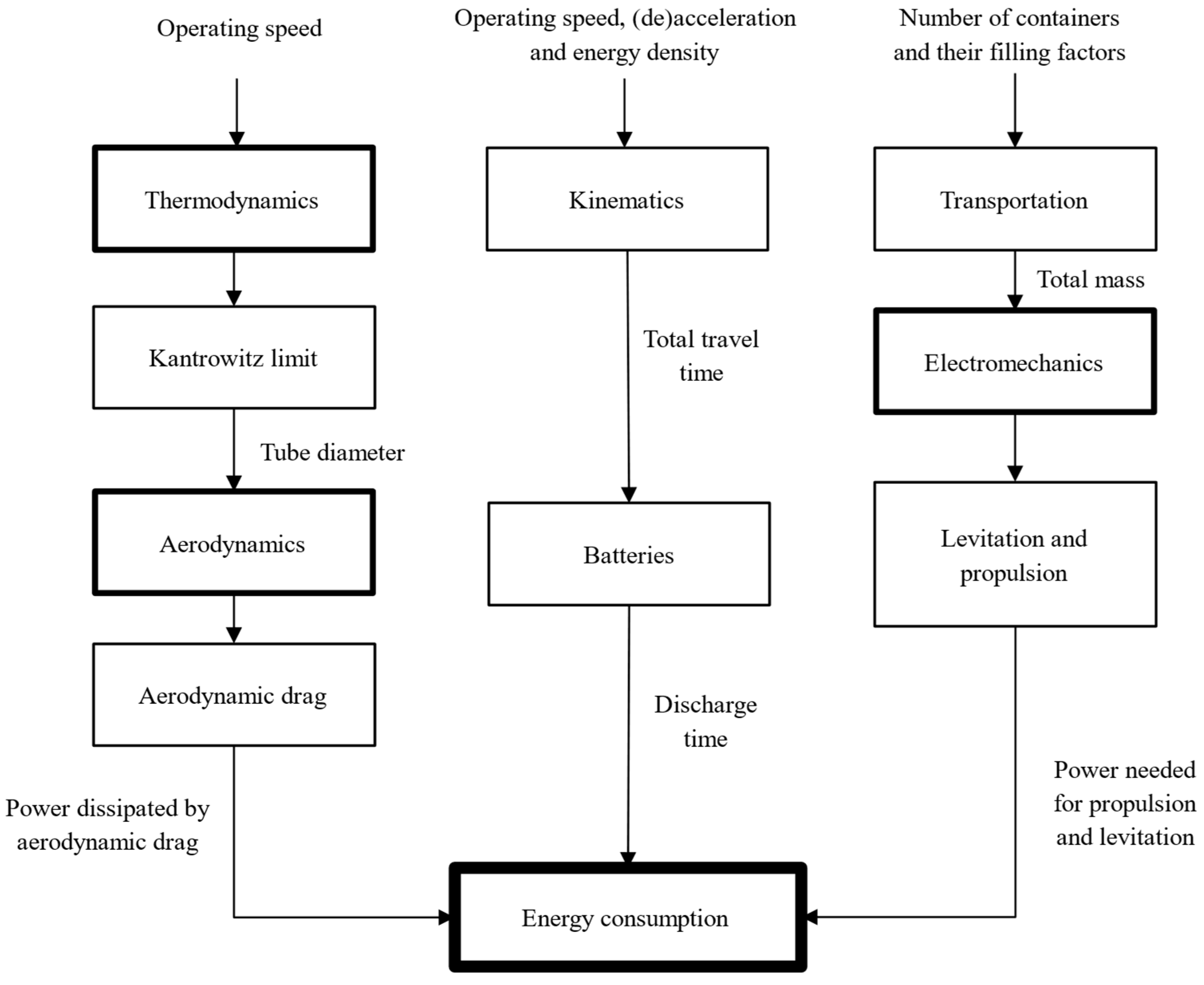
2.2. Calculation Process
- In the left branch, the power dissipated by aerodynamic drag is computed. For that, the speed of the vehicle and its thermodynamic data are entered. At that given speed, the tube diameter is calculated so that the Kantrowitz limit is prevented. According to the blockage ratio, the power dissipated by aerodynamic drag is computed.
- In the middle branch, the onboard batteries which feed the rotor of the linear motor are dimensioned. Their dimensioning comes from evaluating their energy density and their discharge time, which depends on the total travel time. In turn, the total travel time relies on the operating speed, acceleration and deceleration of the vehicle through kinematic relations.
- In the right branch, the power needed to propel and lift the vehicle is calculated. This calculus relies highly on the number of containers (which equals the number of capsules in the vehicle) and their individual masses, which depend on the filling factor of each container. These data determine how much mass is lifted and propelled and, thus, the power needed for that.
2.3. List of Abbreviations
2.4. System Definition
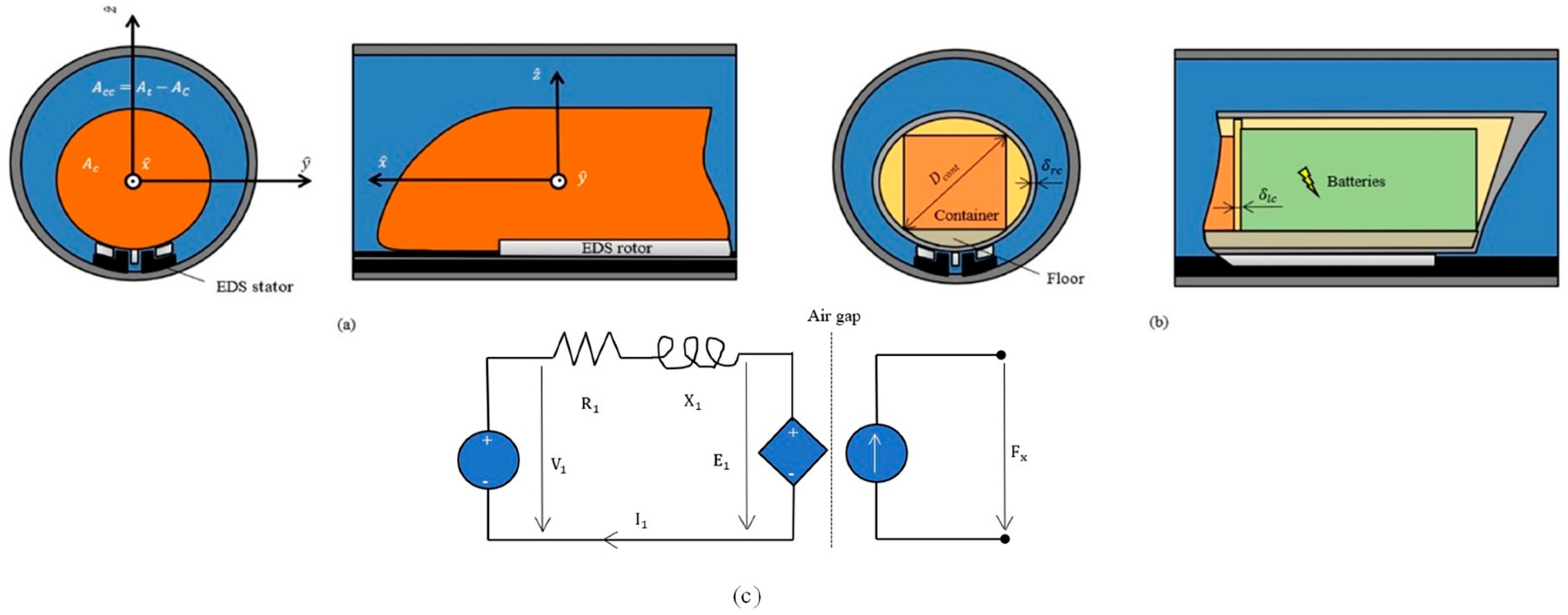
2.4.1. System Drawings
2.4.2. Aerodynamics
2.4.3. Electromechanics
2.4.4. Thermodynamics
2.4.5. Auxiliary Equation Blocks
2.4.6. Final Equation Block
2.5. Software Choice
2.6. Simulation Procedures
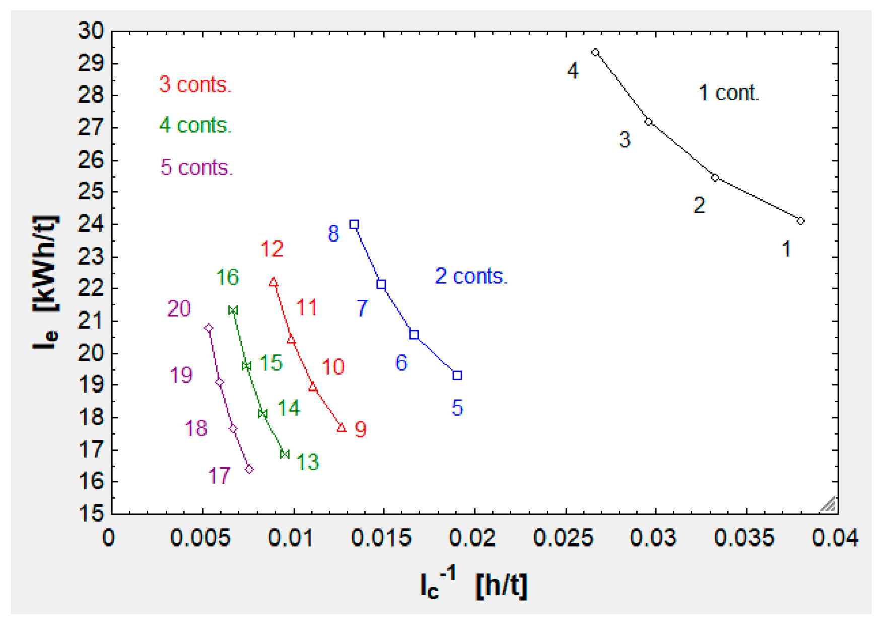
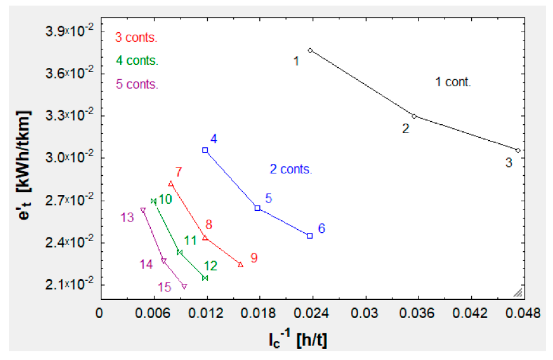
- or, in other words, specific energy consumption to payload, must be the lowest possible.
- or cargo throughput per unit time must be the highest possible. However, its inverse is used on the plot so that optimal points will fall around the lower-left corner. Seen from another perspective, it can be stated that it is important to minimize the time required to send the payload.
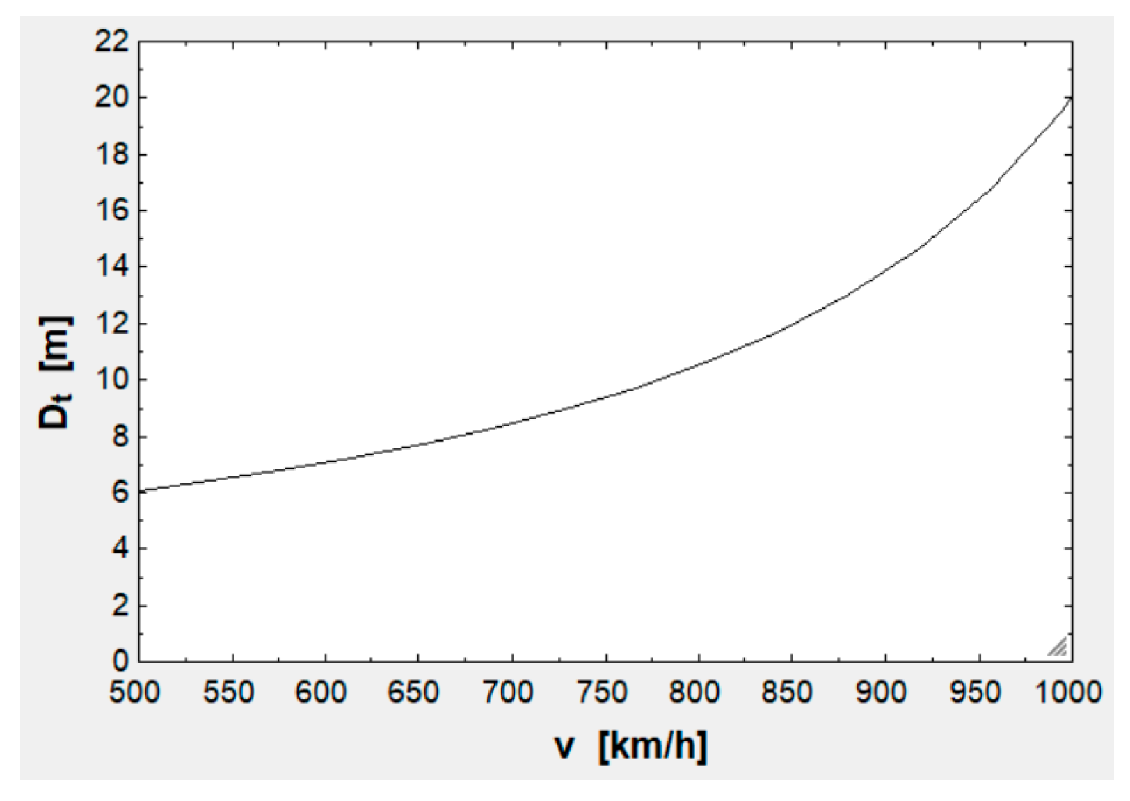
- Speed, which is a relevant factor, as both and strongly depend on it, so a range of speed values is included as input to make the plot. Were the range not included, then the outcome would be one point with coordinates () for every number of containers. The range for a high-speed transportation system without a compressor is 700–1000 km/h, as it will be demonstrated later.
- Tube length. As defined in the beginning, it can take one of three discrete values: 500, 750 or 1000 km. and also depend on this to a great extent.
2.7. Input Data
- (1.5 g). This is because cargo withstands higher accelerations than passengers, as there are not any discomfort issues.
- and are constants and the former is null (there is not any wind flowing inside the tube).
- , R, and were extracted from various references.
- The rest were extracted from a reference in which they were optimized.
3. Results
3.1. Curves
3.2. Curve
3.3. Curves
3.4. Definitive Results
4. Discussion
- measures 9.37 m and is too large because this vehicle lacks an instrument (such as a compressor) to bypass the incoming air. This also impacts speed, since a high-speed transportation system equipped with a compressor is able to reach higher speeds. This last case, in which the vehicle levitated on air bearings instead of magnets, was studied in [24] as an alternative and it was found that this type of vehicle cannot transport a huge amount of freight because maximum mass flow through the compressor limits pressure under the air bearings and, therefore, payload. Nonetheless, a high-speed transportation system with a compressor levitating on magnets has not yet been studied and is proposed for further works. Moreover, it should also be studied whether, or not, it is feasible to build a 9-m diameter tube.
- It should be determined if it is feasible to build a 750 km long EDS or if it would be preferrable to build only some sections of it (the vehicle would cruise between those sections, as proposed by [17]).
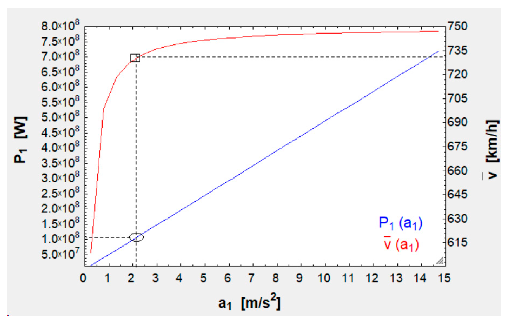
- At the ends, near the cargo terminals (at the acceleration and deceleration lengths), this EDS system should be able to withstand 720 MW ( in Table 3) and evacuate the generated heat (194.40 MW, 27%, because ). State-of-the-art EDS systems are not likely to withstand such an enormous power. In this case, the first approximation done in this work should be discarded and acceleration reduced. If, for instance, 2.10 (1/7 of 14.72) were to be used, its power would be 103 MW, a result which nears the result of reference [17]: 50 MW is the traction power for his first model [17] and for his second model it is 87 MW. The mean speed would barely be affected, as it would only be reduced from 747 to 730 km/h. This can be previewed on the next plot (Figure 7), although the optimization of acceleration and EDS power should be deeply studied, so they are two topics proposed for further studies:Figure 7. Correlations between and and between and . At 2.0 m/s2, and .
![Algorithms 17 00017 g007]()
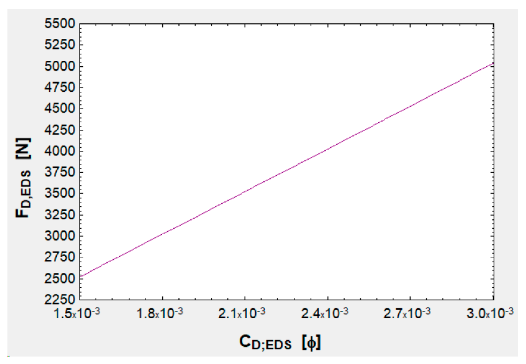
- In addition to the optimization of EDS power, the pole pitch should be adjusted to have or even lower. Thanks to such a good coefficient is only 5 kN (very low in comparison with , which is greater than 1.5 MN), and this drag force can further be lowered, as is shown in Figure 8:Figure 8. Correlation between and , the latter 5 kN at .
![Algorithms 17 00017 g008]()
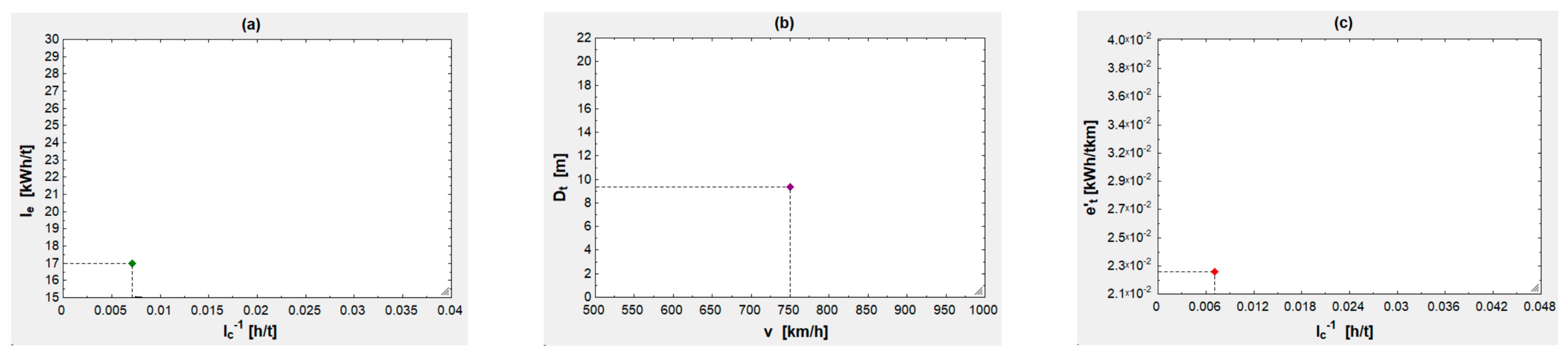
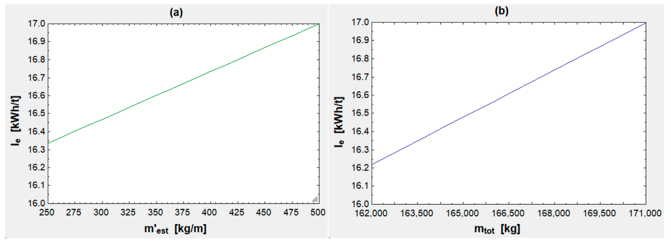
- An attempt to lower , which is the main dead weight of the vehicle, could also be carried out. Nowadays, there are many composite materials reinforced with advanced fibers (carbon-graphite, aramid, etc.) and alloys (aluminum alloys, for instance) which could lighten the vehicle while resisting the stresses and forces generated. If the structure weight could be lowered by 50%, then the energy index could be cut by 3.88% (Figure 9a), and the energy saving could be further augmented to 4.59% by cutting the rest of dead weight (namely, and ) in half also (Figure 9b):Figure 9. (a) Correlation between and . (b) Correlation between and . The latter is 17 kWh/t at kg/m and can be reduced by eliminating some dead weight, as indicated in the text.Figure 9. (a) Correlation between and . (b) Correlation between and . The latter is 17 kWh/t at kg/m and can be reduced by eliminating some dead weight, as indicated in the text.
![Algorithms 17 00017 g009]()
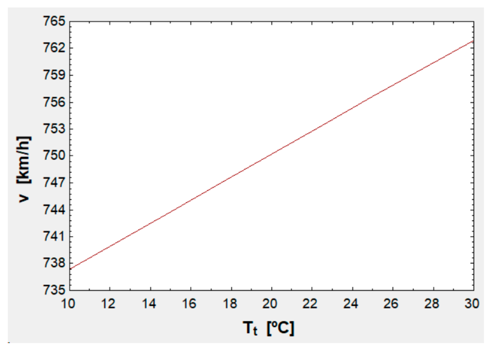
- With respect to the Kantrowitz limit, the vehicle is meant to run at 750 km/h in a 9.37-m diameter tube and at 20 °C. At 30 °C, speed could be slightly raised and at 10 °C speed should be slightly diminished to avoid the air stacking. These possible slight variations are illustrated in Figure 10:Figure 10. Correlation between and . At the operating point, and and when varies, the operating speed can be raised or lowered.Figure 10. Correlation between and . At the operating point, and and when varies, the operating speed can be raised or lowered.
![Algorithms 17 00017 g010]()
- In relation with the previous point, it must be noted that, if this high-speed transportation system were to run in extremely high or low temperature environments, then speed should be diminished or augmented, respectively, although a redesigning process would be more efficient.
- As for the feasibility of keeping airtightness at 250 Pa, it should also be studied, though it is presumably more feasible than 100 Pa, the pressure proposed by [17]. In relation to this, another proposal is the improvement of through CFD simulation or a wind tunnel.


5. Conclusions
Author Contributions
Funding
Data Availability Statement
Acknowledgments
Conflicts of Interest
Appendix A

| Abbreviation | Definition | Unit (SI) | Abbreviation | Definition | Unit (SI) |
|---|---|---|---|---|---|
| Pod cross-sectional area | Emergency brakes mass | ||||
| Annulus area | EDS magnets mass per unit length | ||||
| Frontal area projected on a plane normal to the tube | Structural mass per unit length | ||||
| Tube cross-sectional area | Batteries mass | ||||
| Acceleration | Mass flow through the tube (relative to vehicle) | ||||
| Deceleration | Tare of one container | ||||
| Sound speed | Vehicle total mass | ||||
| EDS drag coefficient | Number of containers transported | ||||
| Drag coefficient outside the tube | Input power to EDS | W | |||
| Drag coefficient inside the tube | Power dissipated by running resistance | W | |||
| Wind speed induced inside the tube | Power dissipated by aerodynamic drag | W | |||
| Capsule diameter | Power dissipated by EDS drag | W | |||
| Diameter needed to fit the cargo | Power really used for propulsion | W | |||
| Diameter of the circumference surrounding one container | Pressure inside the tube | ||||
| Displacement diameter | Total pressure inside the tube | ||||
| Momentum diameter | Constant for a certain ideal gas | ||||
| Tube diameter | Vehicle running resistance | ||||
| Phase voltage at the stator after losses | Stator resistance | ||||
| Energy consumed during acceleration | Tunnel factor | ||||
| Energy consumed by the batteries | Temperature inside the tube | ||||
| Energy generated during deceleration | Total temperature inside the tube | ||||
| Total energy consumed per unit length | Acceleration time | ||||
| Energy consumed throughout the travel at the speed v | Deceleration time | ||||
| Battery stored energy per unit mass | Batteries discharge time | ||||
| Total energy per unit length and payload mass | Total route time | ||||
| Drag force | Travel time at the speed v | ||||
| EDS drag force | Phase input voltage to the stator | ||||
| Propulsion force (along x axis) | Vehicle operating speed | ||||
| Levitation force (along z axis) | Stator reactance | ||||
| Filling factor of each container (for ) | Blockage ratio | ||||
| Gravity acceleration | Adiabatic index | ||||
| Stator line current | Angle between e | ||||
| Transport capacity per unit time (capacity index) | Displacement section | ||||
| Energy consumption per payload mass (energy index) | Momentum section | ||||
| Acceleration length | Boundary layer displacement thickness | ||||
| Length of one capsule | Pod longitudinal thickness | ||||
| Length of one container | Pod radial thickness | ||||
| Deceleration length | Battery charging efficiency | ||||
| Tube length (same as the route one) | EDS efficiency | ||||
| Travel length at the speed v | Boundary layer momentum thickness | ||||
| Mach number | Density inside the tube | ||||
| Maximum cargo of one container | Percentage of battery duration over travel time | ||||
| Mass flow through the annulus | EDS power angle |
Appendix B
| Block | Equation | Left–Side Variable [SI Unit] | Variable Definition | Equation Number |
|---|---|---|---|---|
| Kantrowitz limit | Annulus area | (A1) | ||
| Tube cross-sectional area | (A2) | |||
| Pod cross-sectional area | (A3) | |||
| Capsule diameter | (A4) | |||
| Mass flow through the tube (relative to vehicle) | (A5) | |||
| Aerodynamic drag | Drag force | (A6) | ||
| Power dissipated by aerodynamic drag | (A7) | |||
| Batteries | Batteries discharge time | (A8) | ||
| Kinematics | Acceleration time | (A9) | ||
| Deceleration time | (A10) | |||
| Mean speed of the vehicle | (A11) | |||
| Total route time | (A12) | |||
| Travel time at the speed v | (A13) | |||
| Acceleration length | (A14) | |||
| Deceleration length | (A15) | |||
| Travel length at the speed v | (A16) | |||
| Levitation and propulsion | Propulsion force (along x axis) | (A17) | ||
| Power really used for propulsion | (A18) | |||
| Vehicle running resistance | (A19) | |||
| Power dissipated by running resistance | (A20) | |||
| Input power to EDS | (A21) | |||
| Transportation | Vehicle total mass | (A22) | ||
| Diameter needed to fit the cargo | (A23) | |||
| Length of one capsule | (A24) | |||
(Note that Equation (A25) is not the traditional capacity equation. This Equation has been specifically engineered for this problem, assuming that only one vehicle is using the tube at a time, i.e., the one which is to be optimized.) | Transport capacity per unit time (capacity index) | (A25) |
Appendix C
| Run | ) | (km/h) | (kg) | (kg) | |||||||||
|---|---|---|---|---|---|---|---|---|---|---|---|---|---|
| 1 | 1 | 1 | 0 | 0 | 0 | 0 | 700 | 350 | 750 | 34,845 | 26.32 | 24.11 | 3.80 × 10⁻² |
| 2 | 1 | 1 | 0 | 0 | 0 | 0 | 800 | 350 | 750 | 34,845 | 30.05 | 25.46 | 3.33 × 10⁻² |
| 3 | 1 | 1 | 0 | 0 | 0 | 0 | 900 | 350 | 750 | 34,845 | 33.77 | 27.19 | 2.96 × 10⁻² |
| 4 | 1 | 1 | 0 | 0 | 0 | 0 | 1000 | 350 | 750 | 34,845 | 37.47 | 29.36 | 2.67 × 10⁻² |
| 5 | 2 | 1 | 1 | 0 | 0 | 0 | 700 | 400 | 1000 | 68,891 | 52.65 | 19.29 | 1.90 × 10⁻² |
| 6 | 2 | 1 | 1 | 0 | 0 | 0 | 800 | 400 | 1000 | 68,891 | 60.10 | 20.58 | 1.66 × 10⁻² |
| 7 | 2 | 1 | 1 | 0 | 0 | 0 | 900 | 400 | 1000 | 68,891 | 67.54 | 22.15 | 1.48 × 10⁻² |
| 8 | 2 | 1 | 1 | 0 | 0 | 0 | 1000 | 400 | 1000 | 68,891 | 74.94 | 24.01 | 1.33 × 10⁻² |
| 9 | 3 | 1 | 1 | 1 | 0 | 0 | 700 | 450 | 1250 | 102,936 | 78.97 | 17.68 | 1.27 × 10⁻² |
| 10 | 3 | 1 | 1 | 1 | 0 | 0 | 800 | 450 | 1250 | 102,936 | 90.16 | 18.95 | 1.11 × 10⁻² |
| 11 | 3 | 1 | 1 | 1 | 0 | 0 | 900 | 450 | 1250 | 102,936 | 101.31 | 20.46 | 9.87 × 10⁻³ |
| 12 | 3 | 1 | 1 | 1 | 0 | 0 | 1000 | 450 | 1250 | 102,936 | 112.41 | 22.23 | 8.90 × 10⁻³ |
| 13 | 4 | 1 | 1 | 1 | 1 | 0 | 700 | 500 | 1500 | 136,986 | 105.29 | 16.88 | 9.50 × 10⁻³ |
| 14 | 4 | 1 | 1 | 1 | 1 | 0 | 800 | 500 | 1500 | 136,986 | 120.21 | 18.14 | 8.32 × 10⁻³ |
| 15 | 4 | 1 | 1 | 1 | 1 | 0 | 900 | 500 | 1500 | 136,986 | 135.08 | 19.62 | 7.40 × 10⁻³ |
| 16 | 4 | 1 | 1 | 1 | 1 | 0 | 1000 | 500 | 1500 | 136,986 | 149.89 | 21.33 | 6.67 × 10⁻³ |
| 17 | 5 | 1 | 1 | 1 | 1 | 1 | 700 | 550 | 1750 | 171,027 | 131.62 | 16.40 | 7.60 × 10⁻³ |
| 18 | 5 | 1 | 1 | 1 | 1 | 1 | 800 | 550 | 1750 | 171,027 | 150.26 | 17.65 | 6.66 × 10⁻³ |
| 19 | 5 | 1 | 1 | 1 | 1 | 1 | 900 | 550 | 1750 | 171,027 | 168.84 | 19.12 | 5.92 × 10⁻³ |
| 20 | 5 | 1 | 1 | 1 | 1 | 1 | 1000 | 550 | 1750 | 171,027 | 187.36 | 20.80 | 5.34 × 10⁻³ |
| Run | Run | (m) | |||||||
|---|---|---|---|---|---|---|---|---|---|
| 1 | 500 | 0.40 | 6.05 | 3.65 × 10⁻¹ | 11 | 880 | 0.71 | 13.02 | 7.90 × 10⁻² |
| 2 | 538 | 0.44 | 6.40 | 3.27 × 10⁻¹ | 12 | 918 | 0.74 | 14.66 | 6.23 × 10⁻² |
| 3 | 576 | 0.47 | 6.78 | 2.91 × 10⁻¹ | 13 | 956 | 0.77 | 16.76 | 4.76 × 10⁻² |
| 4 | 614 | 0.50 | 7.22 | 2.57 × 10⁻¹ | 14 | 994 | 0.80 | 19.52 | 3.51 × 10⁻² |
| 5 | 652 | 0.53 | 7.71 | 2.25 × 10⁻¹ | 15 | 1032 | 0.84 | 23.33 | 2.46 × 10⁻² |
| 6 | 690 | 0.56 | 8.28 | 1.95 × 10⁻¹ | 16 | 1070 | 0.87 | 28.89 | 1.60 × 10⁻² |
| 7 | 728 | 0.59 | 8.94 | 1.68 × 10⁻¹ | 17 | 1108 | 0.90 | 37.78 | 9.37 × 10⁻³ |
| 8 | 766 | 0.62 | 9.70 | 1.42 × 10⁻¹ | 18 | 1146 | 0.93 | 54.24 | 4.55 × 10⁻³ |
| 9 | 804 | 0.65 | 10.61 | 1.19 × 10⁻¹ | 19 | 1184 | 0.96 | 95.00 | 1.48 × 10⁻³ |
| 10 | 842 | 0.68 | 11.69 | 9.78 × 10⁻² | 20 | 1222 | 0.99 | 364.88 | 1.01 × 10⁻⁴ |
| Run | ) | (km) | (kg) | (kg) | (kWh/km) | (kWh/t) | (kWh/tkm) | |||||||
|---|---|---|---|---|---|---|---|---|---|---|---|---|---|---|
| 1 | 1 | 1 | 0 | 0 | 0 | 0 | 500 | 350 | 750 | 1.07 | 18.86 | 3.77 × 10⁻² | 42.20 | 2.37 × 10⁻² |
| 2 | 1 | 1 | 0 | 0 | 0 | 0 | 750 | 350 | 750 | 0.93 | 24.74 | 3.30 × 10⁻² | 28.19 | 3.55 × 10⁻² |
| 3 | 1 | 1 | 0 | 0 | 0 | 0 | 1000 | 350 | 750 | 0.87 | 30.62 | 3.06 × 10⁻² | 21.16 | 4.73 × 10⁻² |
| 4 | 2 | 1 | 1 | 0 | 0 | 0 | 500 | 400 | 1000 | 1.73 | 15.28 | 3.06 × 10⁻² | 84.40 | 1.18 × 10⁻² |
| 5 | 2 | 1 | 1 | 0 | 0 | 0 | 750 | 400 | 1000 | 1.50 | 19.90 | 2.65 × 10⁻² | 56.38 | 1.77 × 10⁻² |
| 6 | 2 | 1 | 1 | 0 | 0 | 0 | 1000 | 400 | 1000 | 1.39 | 24.53 | 2.45 × 10⁻² | 42.33 | 2.36 × 10⁻² |
| 7 | 3 | 1 | 1 | 1 | 0 | 0 | 500 | 450 | 1250 | 2.39 | 14.08 | 2.82 × 10⁻² | 126.60 | 7.90 × 10⁻³ |
| 8 | 3 | 1 | 1 | 1 | 0 | 0 | 750 | 450 | 1250 | 2.07 | 18.29 | 2.44 × 10⁻² | 84.57 | 1.18 × 10⁻² |
| 9 | 3 | 1 | 1 | 1 | 0 | 0 | 1000 | 450 | 1250 | 1.91 | 22.50 | 2.25 × 10⁻² | 63.49 | 1.58 × 10⁻² |
| 10 | 4 | 1 | 1 | 1 | 1 | 0 | 500 | 500 | 1500 | 3.05 | 13.49 | 2.70 × 10⁻² | 168.80 | 5.92 × 10⁻³ |
| 11 | 4 | 1 | 1 | 1 | 1 | 0 | 750 | 500 | 1500 | 2.64 | 17.48 | 2.33 × 10⁻² | 112.76 | 8.87 × 10⁻³ |
| 12 | 4 | 1 | 1 | 1 | 1 | 0 | 1000 | 500 | 1500 | 2.43 | 21.48 | 2.15 × 10⁻² | 84.65 | 1.18 × 10⁻² |
| 13 | 5 | 1 | 1 | 1 | 1 | 1 | 500 | 550 | 1750 | 3.72 | 13.13 | 2.63 × 10⁻² | 211.01 | 4.74 × 10⁻³ |
| 14 | 5 | 1 | 1 | 1 | 1 | 1 | 750 | 550 | 1750 | 3.21 | 17.00 | 2.27 × 10⁻² | 140.95 | 7.09 × 10⁻³ |
| 15 | 5 | 1 | 1 | 1 | 1 | 1 | 1000 | 550 | 1750 | 2.95 | 20.87 | 2.09 × 10⁻² | 105.81 | 9.45 × 10⁻³ |
References
- Bizzozero, M.; Yohei Sato, Y.; Sayed, M.A. Aerodynamic study of a Hyperloop pod equipped with compressor to overcome the Kantrowitz limit. J. Wind Eng. Ind. Aerodyn. 2021, 218, 104784. [Google Scholar] [CrossRef]
- Bose, A.; Viswanathan, V.K. Mitigating the piston effect in high-speed hyperloop transportation: A study on the use of aerofoils. Energies 2021, 14, 464. [Google Scholar] [CrossRef]
- Hyde, D.J.; Barr, L.C.; Taylor, C. Hyperloop Commercial Feasibility Analysis: High Level Overview. Resource Document. 2016. Available online: https://ia801201.us.archive.org/12/items/HyperloopCommercialFeasibilityReport/Hyperloop_Commercial_Feasibility_Report.pdf (accessed on 4 November 2023).
- Tudor, D.; Paolone, M. Operational-driven optimal-design of a hyperloop system. Transp. Eng. 2021, 5, 100079. [Google Scholar] [CrossRef]
- Noland, J.K. Prospects and Challenges of the Hyperloop Transportation System: A Systematic Technology Review. IEEE Access 2021, 9, 28439–28458. [Google Scholar] [CrossRef]
- Kisilowski, J.; Kowalik, R. Displacements of the levitation systems in the vehicle hyperloop. Energies 2020, 13, 6595. [Google Scholar] [CrossRef]
- Bhuiya, M.; Aziz, M.M.; Mursheda, F.; Lum, R.; Brar, N.; Youssef, M. A New Hyperloop Transportation System: Design and Practical Integration. Robotics 2022, 11, 23. [Google Scholar] [CrossRef]
- Lee, J.; You, W.; Lim, J.; Lee, K.S.; Lim, J.Y. Development of the Reduced-Scale Vehicle Model for the Dynamic Characteristic Analysis of the Hyperloop. Energies 2021, 14, 3883. [Google Scholar] [CrossRef]
- Sadegi, S.; Saeedifard, M.; Bobko, C. Dynamic Modeling and Simulation of Propulsion and Levitation Systems for Hyperloop. In Proceedings of the 13th International Symposium on Linear Drives for Industry Applications, Wuhan, China, 1–3 July 2021. [Google Scholar]
- Van Goeverden, K.; Milakis, D.; Janic, M.; Konings, R. Analysis and modelling of performances of the HL (Hyperloop) transport system. Eur. Transp. Res. Rev. 2018, 10, 41. [Google Scholar] [CrossRef]
- Sui, Y.; Niu, J.; Yu, Q.; Cao, X.; Yuan, Y.; Yang, X. Influence of vehicle length on the aerothermodynamic environment of the Hyperloop. Tunn. Undergr. Space Technol. 2023, 138, 105126. [Google Scholar] [CrossRef]
- Seo, Y.; Cho, M.; Kim, D.H.; Lee, T.; Ryu, J.; Lee, C. Experimental analysis of aerodynamic characteristics in the Hyperloop system. Aerosp. Sci. Technol. 2023, 137, 108265. [Google Scholar] [CrossRef]
- Mirza, M.O.; Ali, Z. Numerical analysis of aerodynamic characteristics of multi-pod hyperloop system. Proc. Inst. Mech. Eng. Part G J. Aerosp. Eng. 2023, 237, 1727–1750. [Google Scholar] [CrossRef]
- Khodadadian, A.; Parvizi, M.; Heitzinger, C. An adaptive multilevel Monte Carlo algorithm for the stochastic drift–diffusion–Poisson system. Comput. Methods Appl. Mech. Eng. 2020, 368, 113163. [Google Scholar] [CrossRef]
- Khodadadian, A.; Thagiazadeh, L.; Heitzinger, C. Optimal multilevel randomized quasi-Monte-Carlo method for the stochastic drift–diffusion-Poisson system. Comput. Methods Appl. Mech. Eng. 2018, 329, 480–497. [Google Scholar] [CrossRef]
- Melis, M.J.; Matías, I.D.; Alonso, J.M.; Navarro, J.L.; Tasis, J.L. Diseño de túneles para trenes de alta velocidad. Rozamiento tren-aire-túnel y ondas de presión. Rev. Obras Públicas 2001, 148, 27–44. [Google Scholar]
- Musk, E. Hyperloop Alpha. White Paper. 2013. Available online: https://www.tesla.com/sites/default/files/blog_images/hyperloop-alpha.pdf (accessed on 4 November 2023).
- Schlichting, H. Boundary-Layer Theory, 9th ed.; Springer: New York, NY, USA, 2017. [Google Scholar]
- Lever, J.H. Technical Assessment of Maglev System Concepts, Resource Document. 1998. Available online: https://rosap.ntl.bts.gov›dot›dot_42287_DS1.pdf (accessed on 4 November 2023).
- Flankl, M.; Wellerdieck, T.; Tüysüz, A.; Kolar, J.W. Scaling laws for electrodynamic suspension in high-speed transportation. IET Electr. Power Appl. 2018, 12, 357–364. [Google Scholar] [CrossRef]
- Abdelrahman, A.S.; Sayeed, J.M.; Youssef, M.Z. Hyperloop Transportation System: Control, and Drive System Design. In Proceedings of the IEEE Energy Conversion Congress and Exposition, Portland, OR, USA, 23–27 September 2018. [Google Scholar]
- Bar-Meir, G. Fundamentals of Compressible Fluid Mechanics, Version 0.4.9.8; Published online. 2013. Available online: http://www.bigbook.or.kr/bbs/data/file/bo11/1535291005_vkqPUAtN_Fundamentals_of_Compressible_Fluid_Mechanics_Genick_Bar-Meir.pdf (accessed on 4 November 2023).
- Mattingly, J.D. Elements of Gas Turbine Propulsion, 1st ed.; McGraw-Hill: New York, NY, USA, 1996. [Google Scholar]
- Pellicer, D.S.; Larrodé, E. Conceptual Development, Analysis and Simulation of the Transport Capacity of a Freight Transport Vehicle in Vacuum Tubes at High Speed (Hyperloop Concept). Bachelor’s Thesis, University of Zaragoza, Zaragoza, Spain, 2019. Available online: http://deposita.unizar.es/record/48766 (accessed on 4 November 2023).
- Klein, S.A. Development and integration of an equation-solving program for engineering thermodynamics courses. Comput. Appl. Eng. Educ. 1993, 1, 265–275. [Google Scholar] [CrossRef]
- Tirmizi, S.A.; Gandhidasan, P.; Zubair, S.M. Performance analysis of a chilled water system with various pumping schemes. Appl. Energy 2012, 100, 238–248. [Google Scholar] [CrossRef]
- Shakouri, M.; Ghadamian, H.; Sheikholeslami, R. Optimal model for multi effect desalination system integrated with gas turbine. Desalination 2010, 260, 254–263. [Google Scholar] [CrossRef]
- Çengel, Y.A.; Boles, M.A. Thermodynamics: An Engineering Approach, 8th ed.; McGraw-Hill: New York, NY, USA, 2014. [Google Scholar]
- Biswas, M.M.; Azim, M.S.; Saha, T.K.; Zobayer, U.; Urmi, M.C. Towards Implementation of Smart Grid: An Updated Review on Electrical Energy Storage Systems. Smart Grid Renew. Energy 2013, 4, 122–132. [Google Scholar] [CrossRef]


| Block | Equation | Left-Side Variable (SI Unit) | Variable Definition | Equation Number |
|---|---|---|---|---|
| Energy consumption | Energy consumed during acceleration | (34) | ||
| Energy generated during deceleration | (35) | |||
| Mean power dissipated by running resistance | (36) | |||
| Energy consumed throughout the travel at the speed v | (37) | |||
| Energy consumed by the batteries | (38) | |||
| Total energy consumed per unit length | (39) | |||
| Total energy per unit length and payload mass | (40) | |||
| Energy consumption per payload mass (energy index) | (41) |
| Variable | Value | Refs. | Variable | Value | Refs. |
|---|---|---|---|---|---|
| 14.72 | [N/A] | 2180 | [24] | ||
| 14.72 | [N/A] | 250 | [24] | ||
| 3 × 10⁻³ | [24] | 287 | [28] | ||
| 0.60 | [24] | 8 | [24] | ||
| 0 (const.) | [N/A] | 20 | [24] | ||
| 3.558 | [24] | 1.40 | [28] | ||
| 225 | [29] | 15 | [24] | ||
| 9.81 (const.) | [N/A] | 0.04 | [24] | ||
| 6.058 | [24] | 0.05 | [24] | ||
| 28,300 | [24] | 0.90 | [29] | ||
| ) | * | [24] | 0.73 | [24] | |
| 32 | [24] | 30 | [24] | ||
| 500 | [24] | 30 | [24] | ||
| * | [24] |
| Variable | Value | Variable | Value |
|---|---|---|---|
| 10.51 | 1750 | ||
| 58.38 | 32 | ||
| 10.51 | 500 | ||
| 68.89 | 550 | ||
| 14.72 | 42.64 | ||
| 14.72 | 2180 | ||
| 343.20 | 171,027 | ||
| 3 × 10⁻³ | 5 | ||
| 0.60 | 720 | ||
| 1.07 | 1.20 | ||
| 0 | 150,991 | ||
| 3.658 | 1.05 | ||
| 3.558 | 526 | ||
| 3.558 | 250 | ||
| 5.20 | 320.65 | ||
| 4.17 | 287 | ||
| 9.37 | 5758 | ||
| 63,736 | 8 | ||
| 1414.39 | 1.78 | ||
| 105.77 | 20 | ||
| −751.50 | 41.60 | ||
| 3.21 | 14.15 | ||
| 1636.83 | 14.15 | ||
| ) | 225 | 78.31 | |
| 2.27 × 10⁻² | 60.24 | ||
| 724.76 | 59.76 | ||
| 5033.33 | 97,381 | ||
| 2.52 | 750 | ||
| 1.68 | 11.31 | ||
| 1 | ) | 15.26 | |
| 9.81 | 1.40 | ||
| 2846 | 15 | ||
| ) | 140.95 | ) | 10.70 |
| 17 | 3.15 | ||
| 1.47 | 0.77 | ||
| 6.138 | 0.04 | ||
| 6.058 | 0.05 | ||
| 1.47 | 0.90 | ||
| 750 | 0.73 | ||
| 747.05 | 0.26 | ||
| 0.61 | ) | 2.97 × 10⁻³ | |
| 28,300 | 30 | ||
| 42.64 | 30 |
Disclaimer/Publisher’s Note: The statements, opinions and data contained in all publications are solely those of the individual author(s) and contributor(s) and not of MDPI and/or the editor(s). MDPI and/or the editor(s) disclaim responsibility for any injury to people or property resulting from any ideas, methods, instructions or products referred to in the content. |
© 2023 by the authors. Licensee MDPI, Basel, Switzerland. This article is an open access article distributed under the terms and conditions of the Creative Commons Attribution (CC BY) license (https://creativecommons.org/licenses/by/4.0/).
Share and Cite
Pellicer, D.S.; Larrodé, E. Analysis of the Effectiveness of a Freight Transport Vehicle at High Speed in a Vacuum Tube (Hyperloop Transport System). Algorithms 2024, 17, 17. https://doi.org/10.3390/a17010017
Pellicer DS, Larrodé E. Analysis of the Effectiveness of a Freight Transport Vehicle at High Speed in a Vacuum Tube (Hyperloop Transport System). Algorithms. 2024; 17(1):17. https://doi.org/10.3390/a17010017
Chicago/Turabian StylePellicer, David S., and Emilio Larrodé. 2024. "Analysis of the Effectiveness of a Freight Transport Vehicle at High Speed in a Vacuum Tube (Hyperloop Transport System)" Algorithms 17, no. 1: 17. https://doi.org/10.3390/a17010017
APA StylePellicer, D. S., & Larrodé, E. (2024). Analysis of the Effectiveness of a Freight Transport Vehicle at High Speed in a Vacuum Tube (Hyperloop Transport System). Algorithms, 17(1), 17. https://doi.org/10.3390/a17010017