A Geometrical Study about the Biparametric Family of Anomalies in the Elliptic Two-Body Problem with Extensions to Other Families

Abstract

In the present paper, we efficiently solve the two-body problem for extreme cases such as those with high eccentricities. The use of numerical methods, with the usual variables, cannot maintain the perihelion passage accurately. In previous articles, we have verified that this problem is treated more adequately through temporal reparametrizations related to the mean anomaly through the partition function. The biparametric family of anomalies, with an appropriate partition function, allows a systematic study of these transformations. In the present work, we consider the elliptical orbit as a meridian section of the ellipsoid of revolution, and the partition function depends on two variables raised to specific parameters. One of the variables is the mean radius of the ellipsoid at the secondary, and the other is the distance to the primary. One parameter regulates the concentration of points in the apoapsis region, and the other produces a symmetrical displacement between the polar and equatorial regions. The three most used geodesy latitude variables are also studied, resulting in one not belonging to the biparametric family. However, it is in the one introduced now, which implies an extension of the biparametric method. The results obtained using the method presented here now allow a causal interpretation of the operation of numerous reparametrizations used in the study of orbital motion.

1. Introduction

One of the main problems in celestial mechanics is the two-body problem, especially in its elliptical case. This problem can be formulated as follows: given two masses $m_1$, $m_2$ called primary and secondary, respectively, establish the position of the secondary relative to the primary, denoted by $\overrightarrow{r}$, as a function of time.

The second-order differential equations define the relative motion of the secondary with respect to the primary:

$$\frac{d^2\overrightarrow{r}}{d{t}^2}=-\mu \frac{\overrightarrow{r}}{r^3}$$

(1)

where $\overrightarrow{r}$ is the vector radius of the secondary and $\mu =G(m_1+m_2)$, where G is the gravitational constant and $m_1$, $m_2$ the masses of the primary and the secondary, respectively.

The two-body problem in celestial mechanics is a well-known classical integrable problem whose analytical solution is well-known. It has been studied by numerous authors, e.g., [1,2,3,4,5].

This problem is also appropriate for testing numerical methods because we can compare the numerical and the analytical solutions. The analytical solution is described by the set III of elements of Brouwer and Clemence $(a,e,i,\Omega ,\omega ,M)$ [1], where a is the semimajor axis of the ellipse, e the eccentricity, i the inclination, $\Omega$ the argument of ascending node, $\omega$ the argument of the apoapsis, and M the mean anomaly for the epoch.

The performance of the numerical methods is good. However, the distribution of points provided by the natural time is contrary to the dynamics by accumulating more points in the apoapsis region than in the periapsis region if constant time intervals are taken as base points of integration when the opposite would be desirable. One way to achieve this goal is to find a temporal variable for which the distribution of points at constant intervals in the new variables is more significant in the areas of higher speed of the secondary and those with greater curvature. This is particularly interesting in the case of very high eccentricities, like most periodic comets, in whose study numerical integrators can and do present problems.

There are several ways to solve this problem. In this paper, we use the analytical regularization of step size to reparametrize the orbit to obtain a more appropriate point distribution in the orbit. This method can be combined with variable step-size integrators, symplectic integrators, and other techniques. The reparametrization technique is a very interesting method to solve several problems. A review of these methods can be seen in [6].

In 1912, Sundman [7] introduced a change in the temporal variable $\tau$ using the transformation $rd\tau =dt$, a temporal reparametrization of the motion known as the Sundman transformation. In this transformation, we can change the time by the mean anomaly; multiplying by the mean motion n and including in $\tau$ a normalization factor $\frac{1}{a}$, the Sundman transformation can be rewritten as $dg=\frac{r}{a}dM$, where g is the eccentric anomaly. To solve this problem, several authors have tried to use a time transformation to obtain a point distribution more according to the dynamics.

• Hansen [8] pioneered in this field, introducing the relative anomalies.
• Sundman, in 1912 [7], introduced a new temporal variable s related to t by means of $rds=dt$.
• Nacozy [9] introduced a new anomaly $\tau$ related by $r^{\frac{3}{2}}d\tau =dt$.
• Janin and Bond [10,11] extended this transformation to ${\Psi }_{\alpha }$, defined by $r^{\alpha }d{\Psi }_{\alpha }=dt$.
• Brumberg [12] introduced the regularized length of arc $s^{*}$ by $vd{s}^{*}=dt$, where v is the velocity of the secondary.
• Brumberg and Fukushima [13] introduced the elliptic anomaly w as $w=\frac{\pi z}{2K\left(e\right)}-\frac{\pi }{2}$, where $\mathrm{am}z=g+\frac{\pi }{2}$.

This method has been used by several authors to obtain a set of time reparametrizations $\Psi$ of the form $dM=Q\left(r\right)d\Psi$, where $Q\left(r\right)$ is called the partition function and $\Psi =\Psi \left(M\right)$ is a $2\pi$ periodic function of M that satisfies $\Psi \left(0\right)=0$, $\Psi \left(\pi \right)=\pi$.

All these variables can be reduced to anomalies, including a normalization scale factor, so that they take values in $[0,2\pi ]$ along one revolution. The classic mean anomaly M, the eccentric anomaly g, and the true anomaly f can be considered temporal variables. López [14] defines the semifocal anomaly $\Psi$ as the mean between f and $f^{\prime }$, where $f^{\prime }$ is the antifocal anomaly [15].

In the year 2017, López introduced the biparametric family of anomalies ${\Psi }_{\alpha ,\beta }$, defined by López [16] as

$$K_{\alpha ,\beta }{r}^{\alpha }{r}^{\prime \beta }d{\Psi }_{\alpha ,\beta }=dM.$$

(2)

This family contains the anomalies defined by the previous time transformations. For $\alpha =\beta =0$, we have the mean anomaly M; for $\alpha =1$, $\beta =0$, the eccentric anomaly g; for $\alpha =1/2$, $\beta =-1/2$, the generalized length of arc introduced by Brumberg; for $\alpha =3/2$, $\beta =1/2$, the elliptic anomaly w; for $\alpha =1$, $\beta =1$, the antifocal anomaly; and for $\alpha =2$, $\beta =1$, the semifocal anomaly. The biparametric family groups many anomalies used in celestial mechanics, although this is an empirical grouping.

Notice that the anomaly ${\Psi }_{\alpha ,\beta }$ is symmetric to the axis of the ellipse when $\alpha -\beta =1$.

There are some interesting anomalies not included in this biparametric family [17,18,19,20].

This paper is focused on studying a new geometric point of view on the biparametric family, which allows reinterpretation of its operation in causal terms, which would be a relevant fact. This section presents the background and the primary goal of this paper. In Section 2, we study the relation between the curvature of the revolution ellipsoid that contains the orbit and the vector radii r $r^{\prime }$. From them, the biparametric family of anomalies is related through the vector radius r and the mean radius of curvature of the ellipsoid. In Section 3, we study several anomalies induced by the latitudes of the ellipsoid, in particular, the geodetic latitude $\Psi$ and the geocentric latitude $\Phi$, concluding in the first case that the anomaly induced by the geodetic latitude coincides with the semifocal anomaly and the anomaly induced by the geocentric anomaly is not included in the biparametric family of anomalies. Despite the above, we can generalize the relations obtained for the biparametric family to the other anomalies in some instances. In Section 4, we present several numerical examples that allow a better understanding of the results previously obtained. In Section 5, the main conclusions of this study will be discussed.

2. The Biparametric Family of Anomalies as a Function of Vector Radius and  Curvature

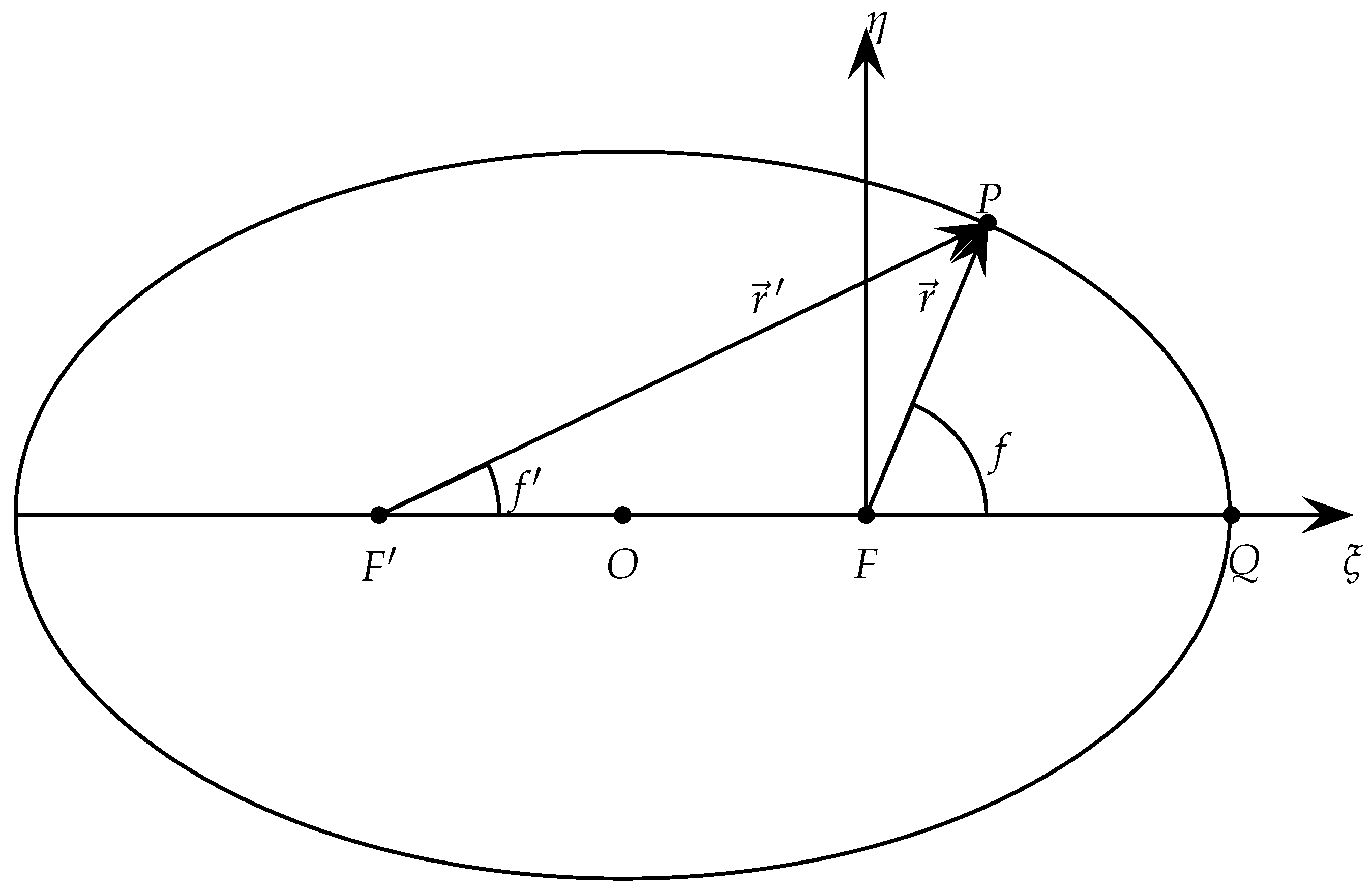
This section studies the relationship between the product of the radii vectors r and $r^{\prime }$ of a point P, which represents the secondary point in the elliptic case of the two-body problem, where r represents the distance to the main focus where the primary is located and $r^{\prime }$ the distance to the secondary focus of the ellipse. These magnitudes are reflected in Figure 1, where the true anomaly f and the antifocal anomaly $f^{\prime }$ also appear. The radii vectors r, $r^{\prime }$, since the orbit is an ellipse, are related by

$$r+r^{\prime }=2a.$$

(3)

Taking into account the relationship between the radius vectors as a function of the eccentric anomaly in the two-body problem and (3), we immediately have:

$$r=a(1-ecosg),r^{\prime }=a(1+ecosg).$$

(4)

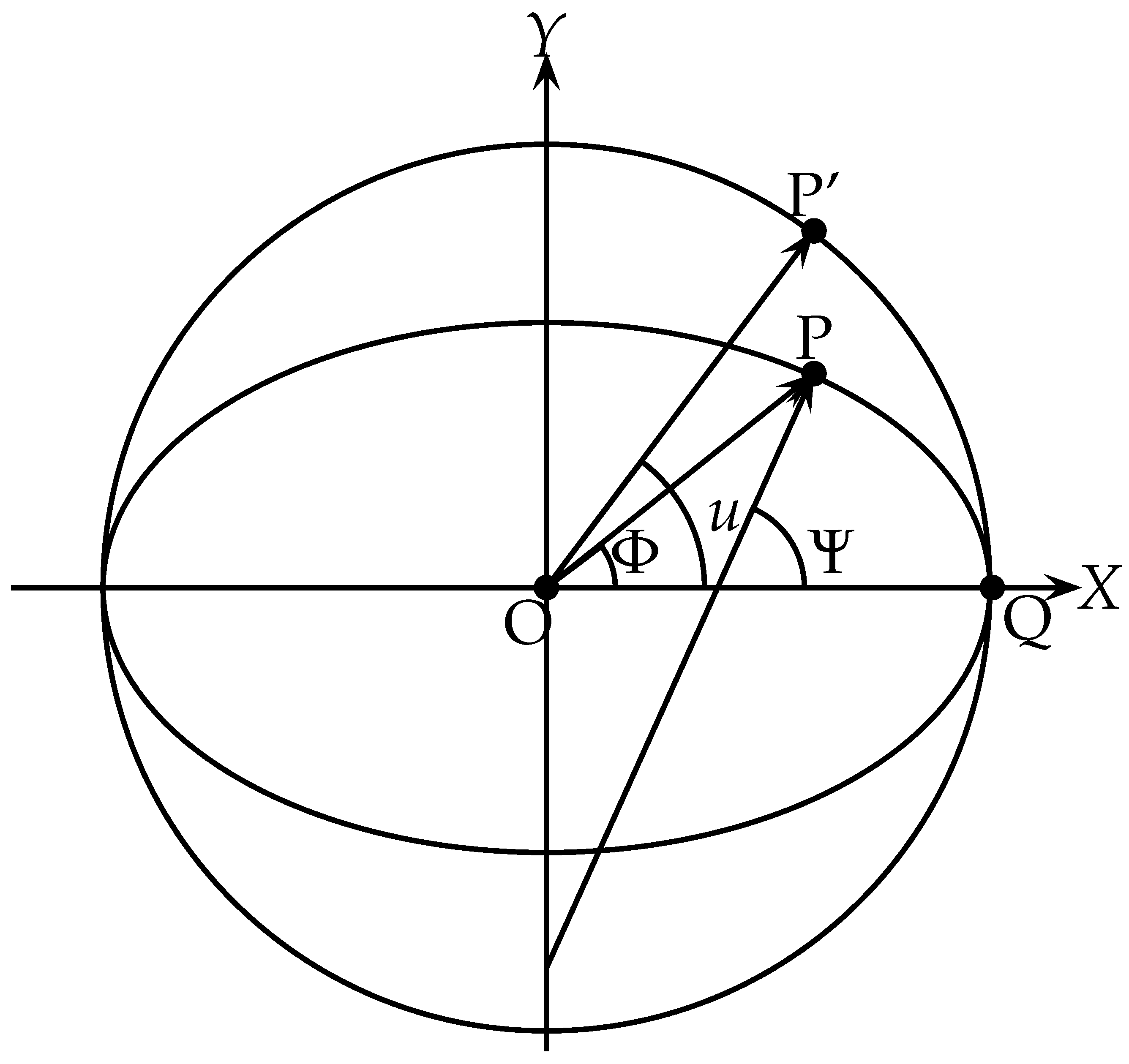
In order to find simple geometric relationships, we will generate an ellipsoid of revolution from the ellipse by rotating the orbit around its semiminor axis. In this ellipsoid, we will take the meridian of zero longitude as the one containing the periapsis of the orbit. It is enough to obtain its longitude and latitude to determine the position of a point P on the ellipsoid. In the case of points located on the orbit whose rotation generates the ellipsoid and the origin of whose length is fixed, it is more convenient to dispense with the length and take a modified length that takes values between $[0,2\pi ]$, which does not present any difficulty and characterizes all the points P on the orbit.

Figure 2 shows the variables u, $\Psi$, and $\Phi$ [4,21], called in geodesy the parametric or reduced latitude, geodesic latitude, and geocentric latitude. When we restrict ourselves to the orbit generated by the ellipsoid, as stated above, we will call them the eccentric anomaly g in the case of u, the geodesic anomaly in the case of $\Psi$, and the geocentric anomaly in the case of $\Phi$. In the next section, it will be shown that the geodetic anomaly coincides with the semifocal anomaly in elliptical motion.

It will be enough to study the main curvature and the mean and Gaussian curvature in the ellipse’s first quadrant for reasons of symmetry. Firstly, given a non-umbilical point P [22] on the first quadrant, we will consider a coordinate system $OXYZ$ so that O is located in the center of the orbit and therefore of the ellipsoid, the axis $OX$ runs to the peripsis, the axis $OY$ is in the direction of the semiminor axis of the ellipse, and the axis $OZ$ forms a direct trihedron with O and $OY$. This notation, which is different from that used in geodesy, is used in celestial mechanics when we take the orbital plane as the $OXY$ plane and place O in the center of the orbit.

The relationship between the different latitudes [4,21] is determined by:

$$\frac{1}{\sqrt{1-e^2}}tan\Psi =tanu=\sqrt{1-e^2}tan\Phi .$$

(5)

In the ellipse that defines the equation of the orbit, the main directions of curvature are given by the direction of the meridian and that of the parallel. In the first case, the ellipse itself is normal to the surface of the ellipse; its curvature will be the main curvature ${\kappa }_1$, and the corresponding radius, which we will denote by ${\rho }_1$, is given by [4,21]:

$${\kappa }_1=\frac{{(1-e^2{sin}^2\Psi )}^{3/2}}{a(1-e^2)},{\rho }_1=\frac{a(1-e^2)}{{(1-e^2{sin}^2\Psi )}^{3/2}}.$$

(6)

On the other hand, the parallel is not a normal section of the ellipsoid. To construct the corresponding normal section, the first vertical must intersect with the ellipsoid, and from their curvatures [4,21], it turns out that:

$${\kappa }_2=\frac{\sqrt{1-e^2{sin}^2\Psi }}{a},{\rho }_2=\frac{a}{\sqrt{1-e^2{sin}^2\Psi }}.$$

(7)

For a normal section whose direction in P has azimuth A measured from the north, it is verified that its curvature and its radius of curvature are given [21] by:

$${\kappa }_A={\kappa }_1{cos}^{2}A+{\kappa }_2{sin}^{2}A,{\rho }_A=\frac{{\kappa }_1{\kappa }_2}{{\kappa }_1{sin}^{2}A+{\kappa }_2{cos}^{2}A}.$$

(8)

It is also of interest to calculate the average curvature ${\kappa }_m$ and the average radius of curvature ${\rho }_m$, which leads to the quantities [21]

$${\kappa }_m=\frac{4}{2\pi }{\int }_0^{\pi /2}{\kappa }_{A}dA=\frac{1}{2}({\kappa }_1+{\kappa }_2).$$

(9)

If, in addition, we average the radii of normal curvatures following directions of different azimuths A at a point P [21], we have that:

$${\rho }_m=\frac{4}{2\pi }{\int }_0^{\pi /2}{\rho }_{A}dA=\frac{4}{2\pi }{\int }_0^{\pi /2}\frac{{\kappa }_1{\kappa }_2}{{\kappa }_1{sin}^{2}A+{\kappa }_2{cos}^{2}A}dA=\sqrt{{\rho }_1{\rho }_2}.$$

(10)

Notice that the relation ${\rho }_m{\kappa }_m=1$ is not satisfied. For this reason and to avoid confusion, we will use the notation $R={\rho }_m$, since, as we have seen, it is not the inverse of the mean curvature.

Taking into consideration the Gaussian curvature of a surface $K(\left(P\right)={\kappa }_1\left(P\right){\kappa }_2\left(P\right)$, which is an intrinsic magnitude, a result known as Gauss’s theorem egregium [22], we have that $R\sqrt{K\left(P\right)}=1$ and, therefore, defining $\kappa$ as

$$\kappa =\sqrt{K\left(P\right)}$$

(11)

it is verified that

$$R=\frac{1}{\kappa }.$$

(12)

To obtain the mean radius of curvature R as a function of the geodetic latitude, just replace (6) and (7) in (10), from which we obtain:

$$R=\frac{a\sqrt{1-e^2}}{1-e^2{sin}^2\Psi }.$$

(13)

On the other hand, as will be seen in the next section, the geodetic latitude coincides with the semifocal anomaly. Therefore, the sine of the latitude $\Psi$ is expressed as a function of the eccentric anomaly g [14] as:

$$sin\Psi =\frac{sing}{\sqrt{1-e^2{cos}^{2}g}}.$$

(14)

Replacing (14) in (13), we have:

$$R=\frac{a(1-e^2{cos}^{2}g)}{\sqrt{1-e^2}}.$$

(15)

Finally, we obtain that the product of the radius vectors r and $r^{\prime }$ given by (4) is given by:

$$r{r}^{\prime }=a^2(1-e^2{cos}^{2}g).$$

(16)

Comparing this last expression with (15), we obtain the fundamental relation:

$$r{r}^{\prime }=a\sqrt{1-e^2}R$$

(17)

Given an anomaly in the biparametric family (2) ${\Psi }_{\alpha ,\beta }$, we can define an equivalent anomaly ${\Phi }_{\gamma ,\delta }$ whose relationship to the mean anomaly is given by:

$$dM=C_{\gamma ,\delta }{r}^{\gamma }{R}^{\delta }d{\Phi }_{\gamma ,\delta },$$

(18)

where $\gamma =\alpha -1$, $\delta =\beta$, $C_{\gamma ,\delta }=a^{\beta }{(1-e^2)}^{\beta /2}{K}_{\alpha ,\beta }$.

In this way, we have the anomaly ${\Phi }_{\gamma ,\delta }={\Psi }_{\alpha ,\beta }$ but whose connection with the mean anomaly is given by (18), where a normalization constant appears. The radius vector r is raised to an exponent $\gamma$ times the mean radius of curvature of the ellipsoid of revolution that contains the orbit as a meridian ellipse R raised to $\delta$. This fact is of great importance because of the effect that the factor $r^{\gamma }$ causes when we work with a constant step number, namely, a translation of the points from the apoapsis region, in the case of working with M, to more concentrated points in the periapsis region; it is more remarkable as $\gamma$ increases. In the case of $\gamma =1$, we are faced with a symmetrical anomaly with respect to the axes of the orbital ellipse.

The second factor $R^{\delta }$ transfers a set of points symmetrical to the axes of the orbital ellipse towards the intersections of the ellipse with the semimajor axis a if $\delta$ is positive and towards the intersection of the ellipse with its semiminor axis if $\delta$ is negative.

As the numerical examples section shows, this allows a purely geometric explanation in the biparametric family of anomalies.

3. Other Symmetric Variables Not Belonging to the Biparametric Family

This section shows that some symmetric variables cannot be included in the modified biparametric family defined above. First, the study of three temporal variables related to the latitudes used in geodesy is addressed to do this. We will consider an ellipsoid of revolution around the semiminor axis of the ellipse so that the orbit is the meridian ellipse located so that the length of the periapsis is zero. The position of a point P on the orbit is determined by the position of this point on the ellipsoid, so it will be enough to determine its latitude on the ellipsoid. In geodesy, the use of three latitudes is common. These latitudes are reflected in Figure 1: the reduced or parametric latitude u, the geodesic latitude $\Psi$, and the geocentric latitude $\Phi$. The range of latitudes u, $\Psi$, $\Phi$ in geodesy is $[-\pi /2,\pi /2]$, given that in the case of the orbit, we do not consider the second geodetic coordinate, that is, the longitude. In order to represent all the points on the orbit, it is necessary to extend the range of these variables to $[0,2\pi ]$. In this way, we can obtain anomalies from these variables.

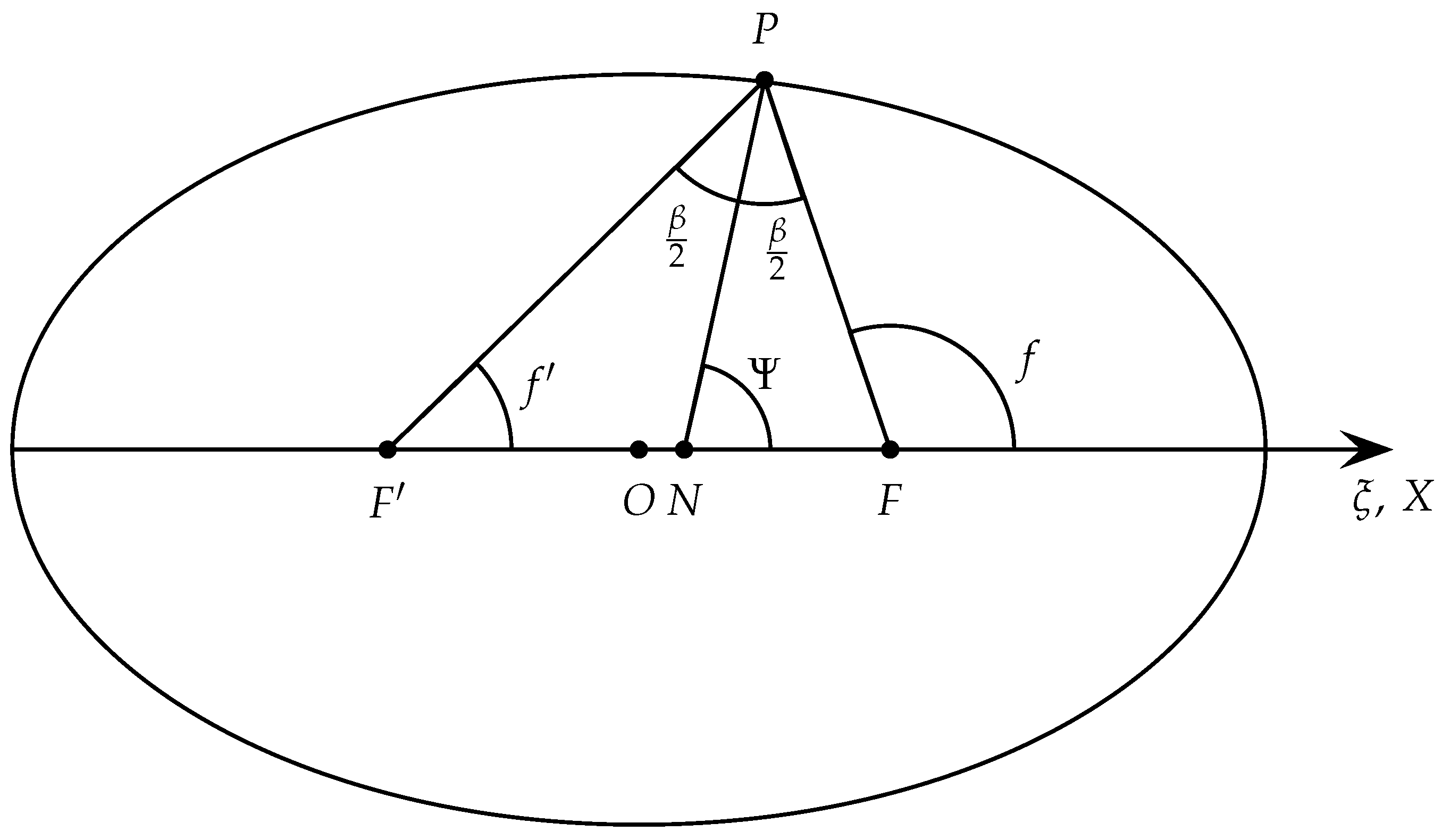
The reduced latitude u is better known as an eccentric anomaly g in celestial mechanics. The geodesic latitude coincides with the semifocal latitude defined by the authors, since a characteristic of the ellipse is the so-called property of elliptical billiards, according to which a ball located at the primary focus, once thrown, bounces off the ellipse and heads to the secondary focus. Therefore, if we consider the point N intersection of the bisector of the angle $\beta$ formed by the radii vectors $\overrightarrow{r}$ and ${\overrightarrow{r}}^{\prime }$ in P, it results that, on the one hand Figure 3, in the triangle of vertices $NFP$, we have that $\pi -f+\beta /2+\Psi =\pi$, and in the triangle of vertices $F^{\prime }PN$ is verified $f^{\prime }+\beta /2+\pi -\Psi =\pi$, from which, eliminating $\beta$, we have $\Psi =\frac{f+f^{\prime }}{2}$. The third latitude variable is the geocentric latitude $\Phi$, which gives rise to a new symmetric anomaly that we will call the central anomaly. Since the radii r, $r^{\prime }$ are, according to the property of elliptical billiards, reflected from each other in the ellipse, the direction $\overrightarrow{PN}$ is normal to the ellipse and therefore $\Psi$ coincides with the geodetic latitude. The semifocal latitude, although it belongs to the biparametric family, will be simply denoted by $\Psi$ instead of ${\Psi }_{2,1}$, as it does not lead to confusion and simplifies the notation.

On the other hand, as is well known, the coordinates of the secondary with respect to the primary $(\xi ,\eta )$ are given by:

$$\xi =a(e-cosg),\eta =a\sqrt{1-e^2}sing,$$

(19)

and the distances between the primary and secondary foci by (4).

Many classical authors have studied the eccentric anomaly [1,2,5], among others. The semifocal anomaly, which, for the reasons explained above, we will also call the geodesic anomaly, has also been studied by [14,23]. At this point, it remains to study the central anomaly $\Phi$. To do this, let $\rho$ be the distance $\overline{OP}$, which is determined by the coordinates of the point P with respect to the system of axes $XY$ with origin in O. Thus, we have:

$$X=\rho cos\Phi ,Y=\rho sin\Phi ,$$

(20)

Depending on the eccentric anomaly, we have $\Phi$. For this, let $\rho$ be the distance $\overline{OP}$, which is determined by the coordinates of the point P with respect to the axis system $XY$ with origin in O; thus, we have:

$$X=acosg,Y=bsing,$$

(21)

where a, $b=a\sqrt{1-e^2}$ are the semimajor and semiminor axes of the ellipse. From the previous equation, we have:

$$\rho =a\sqrt{1-e^2{sin}^{2}g}.$$

(22)

On the other hand, from the equation of the ellipse $\frac{X^2}{a^2}+\frac{Y^2}{b^2}=1$, $\rho$ is obtained as a function of $\Phi$ as:

$$\rho =\frac{a\sqrt{1-e^2}}{\sqrt{1-e^2{sin}^2\Phi }}.$$

(23)

From (20), (21), and (22), it follows that:

$$cos\Phi =\frac{cosg}{\sqrt{1-e^2{sin}^{2}g}},sin\Phi =\frac{\sqrt{1-e^2}sing}{\sqrt{1-e^2{sin}^{2}g}}.$$

(24)

From this equation, and after some elemental calculations, we obtain:

$$cosg=\frac{\sqrt{1-e^2}cos\Phi }{\sqrt{1-e^2{cos}^2\Phi }},sing=\frac{sin\Phi }{\sqrt{1-e^2{cos}^2\Phi }}.$$

(25)

From (24) or (25), we immediately have:

$$tang=\frac{tan\Phi }{\sqrt{1-e^2}}.$$

(26)

Deriving (26), and after some calculations, we have:

$$dg=\frac{1-e^2{sin}^{2}g}{a^2\sqrt{1-e^2}}d\Phi ,$$

(27)

and taking into account (22), the following relationship is obtained:

$$dg=\frac{{\rho }^2}{a^2\sqrt{1-e^2}}d\Phi .$$

(28)

and considering Kepler’s equation for the eccentric anomaly:

$$M=g-esing,$$

(29)

where M is the mean anomaly. It is obtained by derivation:

$$dM=(1-ecosg)dg,$$

(30)

Finally, from (30), (28), and (4), we obtain:

$$dM=\frac{r{\rho }^2}{a^3\sqrt{1-e^2}}d\Phi ,$$

(31)

where, from (22) and (31), the partition function $Q\left(r\right)=\frac{r{\rho }^2}{a^3\sqrt{1-e^2}}$, and after some calculations, we can express $Q\left(r\right)$ as:

$$Q\left(r\right)=\frac{r}{a}\frac{2-e^2}{\sqrt{1-e^2}}-\frac{r{r}^{\prime }}{a^2\sqrt{1-e^2}}=\frac{r}{a\sqrt{1-e^2}}\left[2-e^2-\frac{r(2a-r)}{a^2}\right].$$

(32)

It is evident that the central anomaly $\Phi$ is not in the biparametric family of anomalies. This is not new, since the intermediate radials of Cid [17], the natural family of anomalies [19], and the geometric family of anomalies [20] are not in general in the biparametric family, but they are in the symmetrical case since they coincide, respectively, with the semifocal anomaly and with the eccentric anomaly. Therefore, we have a symmetrical anomaly that does not belong to the biparametric family.

However, it is possible to represent (32) in the form:

$$Q\left(r\right)=\frac{r}{a}\left[\frac{2-e^2}{\sqrt{1-e^2}}-\frac{r{r}^{\prime }}{a^2\sqrt{1-e^2}}\right]=r\left[\frac{2-e^2}{a\sqrt{1-e^2}}-\frac{R}{a^2}\right],$$

(33)

from which we have $Q\left(r\right)=rh\left(R\right)$, where $h\left(R\right)$ is a function of R given by $h\left(R\right)=\frac{2-e^2}{a\sqrt{1-e^2}}-\frac{R}{a^2}$.

This fact can be generalized to $\Theta$ reparameterizations:

$$dM=r^{\gamma }h\left(R\right)d\Theta ,$$

(34)

where the partition function can be written as the product of a power of r times a function of the mean radius of curvature of the ellipsoid of revolution generated by the orbital ellipse. Note that, on the one hand, the normalization factor has been included in the function h and, on the other hand, $dM=Q\left(r\right)d\Theta$ must be an admissible reparametrization.

As a final consideration in this section, it should be noted that $r^{\delta }$ plays the same role as in the case of symmetric anomalies and $h\left(R\right)$ plays a role similar to that of $R^{\delta }$. However, in the latter case, there are more types of symmetrical motions of the points with respect to the semi-axes than those given by the term $R^{\delta }$, which appears in the case of the biparametric family.

4. Numerical Examples

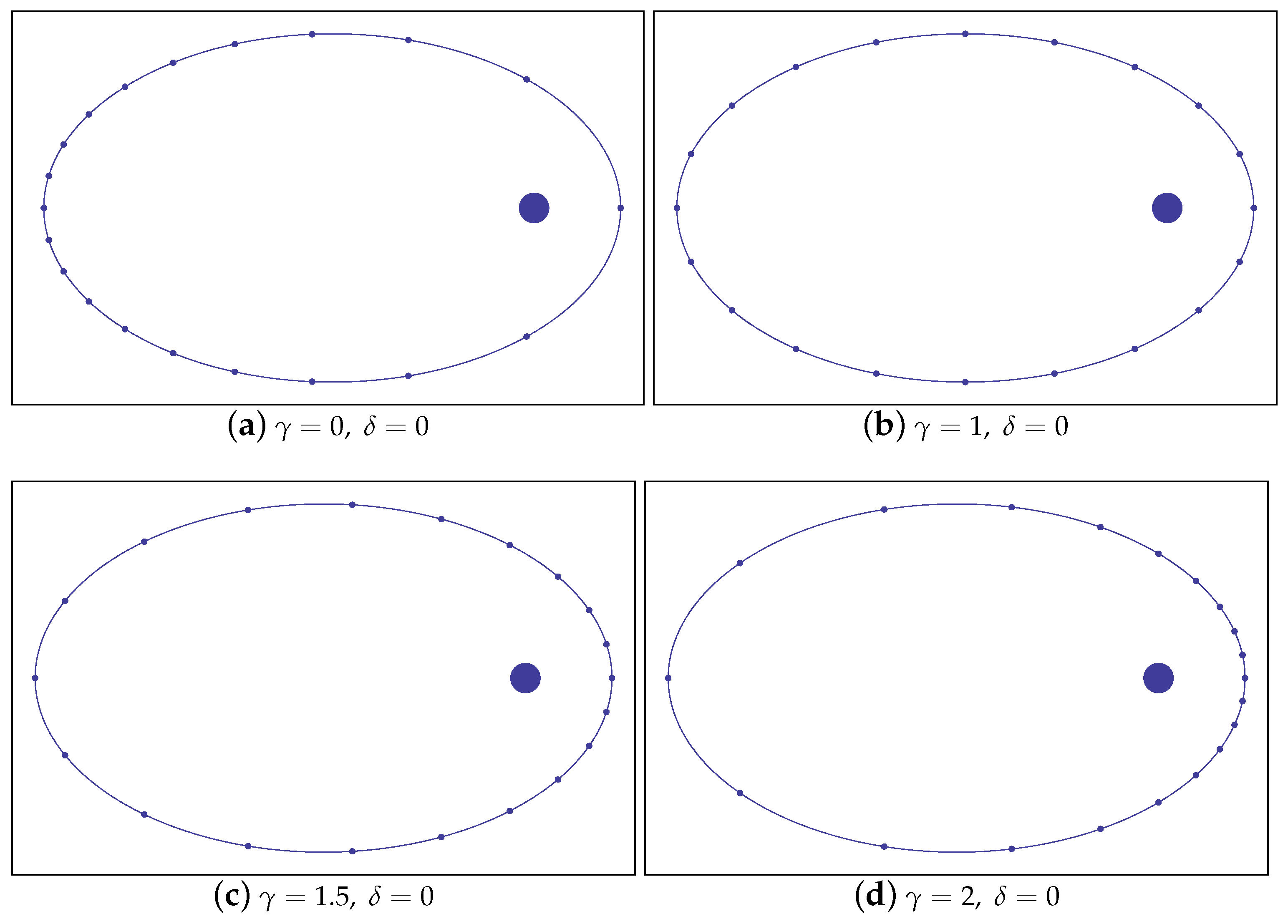
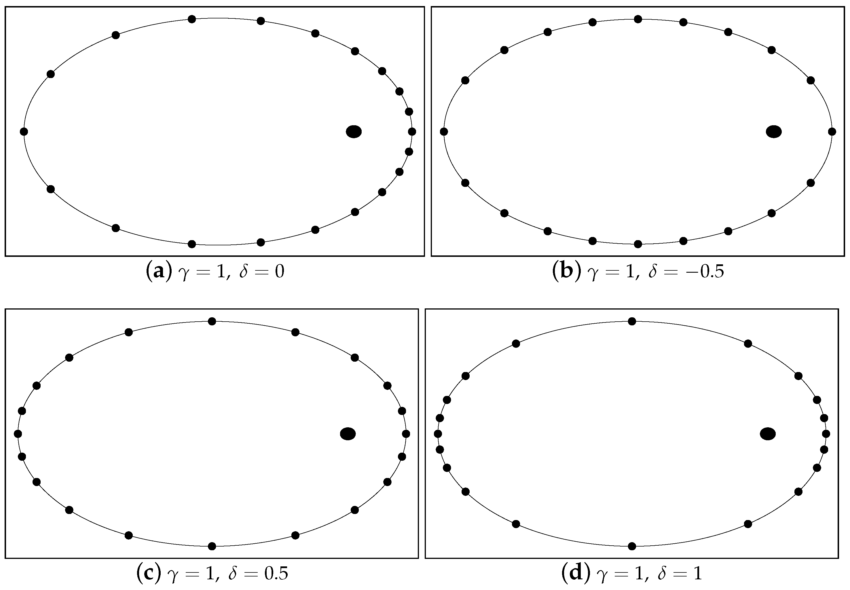
To illustrate the previously obtained results with respect to the new geometric interpretation that transforms the anomaly ${\Psi }_{\alpha ,\eta }$ into its equivalent ${\Phi }_{\gamma ,\delta }$ we will first proceed to represent a set of 20 equally spaced points ${\Phi }_{\gamma ,\delta }$. For this, we will take as an example a satellite with eccentricity $e=0.7$ and M corresponding to $\gamma =0$, $\delta =0$; g corresponding to $\gamma =1$, $\delta =0$; $\tau$ corresponding to $\gamma =1.5$, $\delta =0$; and f corresponding to $\gamma =1.5$, $\delta =0$.

In Figure 4, it can be seen that the factor $r^{\gamma }$ causes a displacement of points from the region corresponding to the apoapsis, that is, from the left part of the ellipse to the region of the periapsis, the right part of the ellipse. This fact implies a distribution of points more in line with the dynamics, which is reflected in better integration values.

Secondly, if the value of $\gamma$ is fixed, we will focus on the example in Figure 5 in the case $\gamma =1$ corresponding to symmetric anomalies. This choice is to show the action of $\gamma$ more clearly.

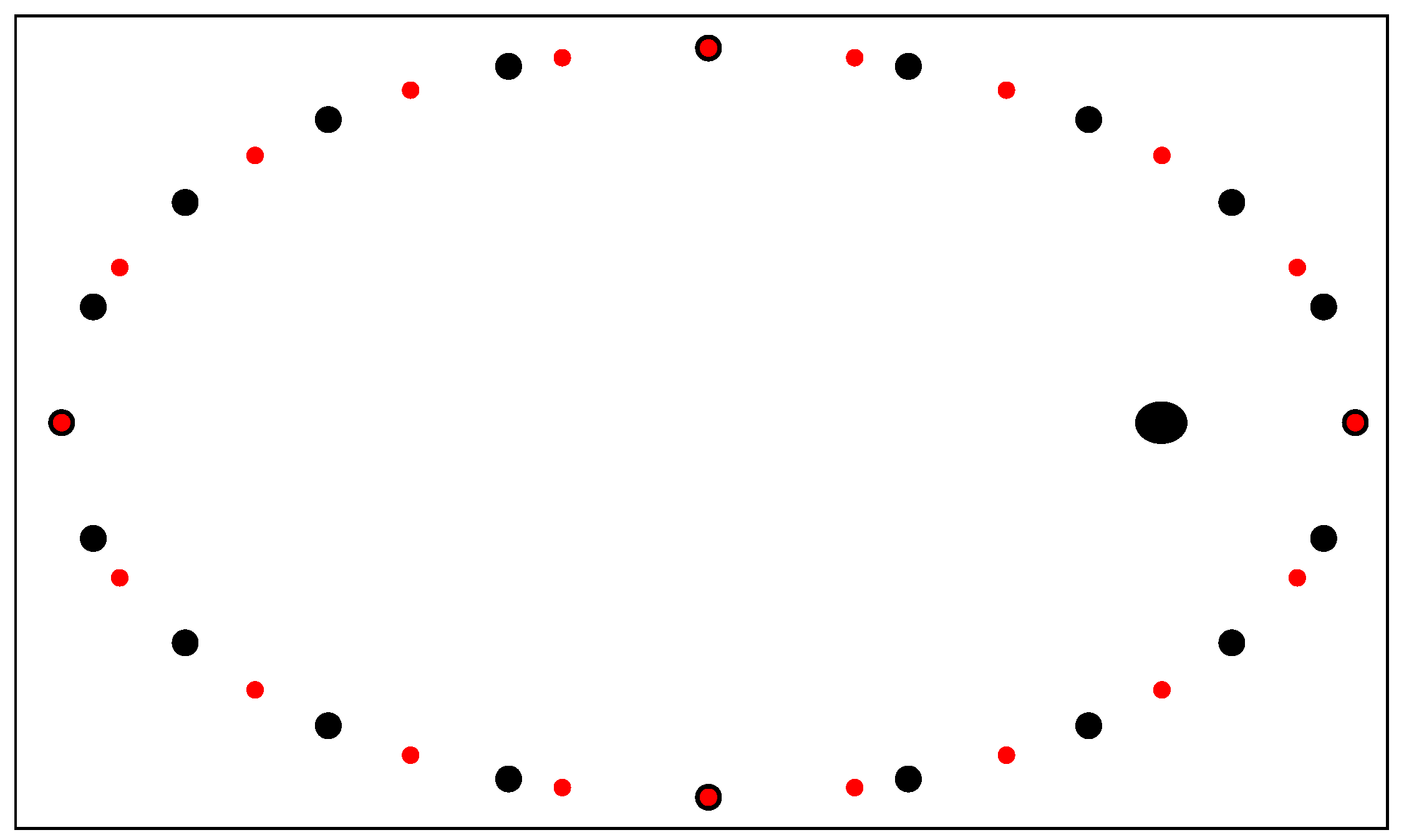
Also, in Figure 6, twenty uniformly distributed points for the eccentric anomaly and the central anomaly are presented on the same graph, and it can be seen that the big black points are more concentrated towards the periapsis and apoapsis regions than those corresponding to the central anomaly. The smaller red dots are more concentrated in the regions corresponding to the intersection of the orbit with respect to the semiminor axis, so it is expected that for large eccentricities, the central anomaly will provide worse precision in the study of orbital motion than the eccentric anomaly.

To interpret the effect on the errors in numerical integration, we proceed to integrate the old artificial satellite Heos II, which is performed in order to compare our results with those of other authors cited above who used this satellite as a test. The satellite’s orbital elements are given by $a=118,363.47$ km, $e=0.942572319$, $i=28°$.16096, $\Omega =185°$.07554, $\omega =270°.07151$, $M0=0°$. The period of the satellite is $4.69$ days and for the Earth the spaceflight constant $\mu =GM=3.986005·{10}^5$ ${\mathrm{km}}^3·$${\mathrm{s}}^{-2}$. Finally, we will analyze the integration errors for various anomalies in the biparametric family according to the new interpretation based on ${\Phi }_{\gamma ,\delta }={\Psi }_{\alpha ,\beta }$.

The results obtained are listed in

Table 1. Integration errors in position (Km) and velocity (Km/s) for different anomalies in the biparametric family ${\Psi }_{\alpha ,\beta }$ and in their equivalents in the representation ${\Phi }_{\gamma ,\delta }$.

	M	g	f	${\mathit{\tau }}^{*}$	${\mathit{s}}^{*}$	w	${\mathit{f}}^{\prime }$	$\mathbf{\Psi }$
$\alpha$	0	1	2	$1.5$	$0.5$	$1.5$	1	2
$\beta$	0	0	0	0	$-0.5$	$0.5$	1	1
$\left|\right|\Delta \overrightarrow{r}\left|\right|$	$9.54\times {10}^{+00}$	$1.12\times {10}^{-05}$	$9.49\times {10}^{-10}$	$2.86\times {10}^{-08}$	$4.51\times {10}^{-04}$	$1.07\times {10}^{-07}$	$2.60\times {10}^{+00}$	$8.03\times {10}^{-06}$
$\left|\right|\Delta \overrightarrow{v}\left|\right|$	$7.71\times {10}^{-03}$	$9.01\times {10}^{-09}$	$3.56\times {10}^{-11}$	$2.41\times {10}^{-11}$	$3.64\times {10}^{-07}$	$4.41\times {10}^{-11}$	$2.10\times {10}^{-03}$	$6.51\times {10}^{-09}$
$\gamma$	0	1	2	$1.5$	1	1	0	1
$\delta$	0	0	0	0	$-0.5$	$0.5$	1	1

, which is, in essence, the same Table 1 that appears in [16] corrected, to which the column corresponding to the semifocal anomaly has been added, and the one that has been added in the lower part the values $(\gamma ,\delta )$ corresponding to the respective $(\alpha ,\beta )$.

Table 1 shows the errors regarding the position and initial velocity made in the numerical integration using $10,000$ equally spaced points, taking different anomalies as integration variables. If the table with value $\gamma =0$ is observed, the mean anomaly M and the antifocal anomaly $f^{\prime }$ appear, which are differentiated by the value of $\delta$, which in the case of the mean anomaly takes a value of 0 and in the case of the antifocal anomaly takes a value of 1. It can be seen in Figure 6 that the distribution of points differs in both cases, concentrating more points in the periapsis region, and correspondingly in the apoapsis region in the case of the antifocal anomaly, which is reflected in the results.

In the case of $\gamma =1$, which corresponds to symmetric anomalies, if the eccentric anomaly g is taken as a basis, the regularized arc length $s^{*}$$\delta$ takes the value $-0.5$, which moves the points away from the apsidal regions, causing worse results. In the case of the elliptical anomaly w and the semifocal anomaly $\Psi$, delta takes the values $0.5$ and 1, respectively. It appears that the precision in position and speed improves with respect to the eccentric anomaly g, which corresponds to a greater concentration of points in the apsidal regions, with the values being better in the case of w. It can be understood that for large values of $\delta$, too many points have been removed over the region corresponding to the ellipse intersection with its semiminor axis, causing a certain loss of precision.

5. Concluding Remarks

In the present study, the relationship between the curvature of a point P of the orbit with the main curvatures of an ellipsoid of revolution generated by the rotation of the orbital ellipse around its semiminor axis has been addressed from a strictly geometric point of view.

Geometric geodesy studies in depth, as a preliminary topic, the geometry of the ellipsoid of revolution, resulting that at a point P, the directions of the main curvature are given by the curvature of the meridian ellipse that passes through the point ${\kappa }_1$ and the normal direction of the parallel to the ellipsoid that passes through the given point. Since the parallel is not normal to the surface of the ellipsoid, the second principal curvature ${\kappa }_2$ is determined by the intersection curve between the first vertical that passes through the point P and the ellipsoid. The inverses of the principal curvatures determine the radii of the main curvatures ${\rho }_1$ and ${\rho }_2$. From these curvatures and given a direction in P of geodesic azimuth A, we have, without further ado than applying classical theory, the curvatures of the normal sections in P, ${\kappa }_A$ according to the directions corresponding to the different azimuths, as well as the corresponding radii of normal curvature ${\rho }_A$. The expressions for the curvatures and radii of curvature above are somewhat complicated, as they contain fractional exponents.

Next, the mean curvature is obtained as an integral mean of the normal curvature with respect to the different azimuths and the average radius of curvature, as well as an integral mean with respect to the different azimuths. The mean curvature and the mean radius of curvature are not inverse, so for simplicity and convenience, R is denoted by the mean radius of curvature, whose $R^2$ turns out to be the inverse of the Gaussian curvature $\kappa ={\kappa }_1{\kappa }_2$, an expression in which fractional powers no longer appear in its latitude-dependent part. The calculation of the product of the radius vectors $r{r}^{\prime }$ leads to an expression directly proportional to R, so that the partition function of the biparametric family of anomalies $Q\left(r\right)=K_{\alpha ,\beta }{r}^{\alpha }{r}^{\prime \beta }$ can be written as $Q\left(r\right)=C_{\gamma ,\delta }{r}^{\gamma }{R}^{\delta }$, where $\gamma =\alpha -1$ and $\delta =\beta$, which appears perfectly factored with respect to the radius vector of the secondary with respect to the primary r and the average radius of curvature of the ellipsoid at point P.

On the other hand, in geodesy, three latitudes are used: the parametric latitude u, the geodetic latitude $\Psi$, and the geocentric latitude $\Psi$, which can be modified for a meridian ellipse by making its value oscillate between $[0,2\pi ]$, thus making u coincide with the eccentric anomaly g. The geodetic latitude is shown to coincide with the semifocal anomaly, and the modified geocentric latitude $\Phi$ does not coincide with any of the known anomalies and is defined as a central anomaly. Once a sufficiently complete study of this variable has been carried out, we obtain the relationships between $\Phi$ and the eccentric anomaly g in closed form. The partition function that relates the anomaly $\Phi$ to the mean anomaly M is also obtained.

One of the first results observed is that said anomaly, which is obviously symmetrical, does not belong to the biparametric family of anomalies. Despite this, it is possible to factorize the partition function as a function proportional to $r·h\left(R\right)$, which allows an interpretation similar to that of the anomalies of the biparametric family, which allows the method to be extended to anomalies whose function of partition is proportional to $r^{\alpha }h\left(R\right)$, provided that they constitute an admissible reparametization of the ellipse.

In the numerical examples section, the effect of $\gamma$ and $\delta$ is observed for the case of the biparametric family. The factor $r^{\gamma }$ causes a translation of the points from the apoapsis region to the periapsis region when a set of equally spaced points is taken in the corresponding anomaly. This translation is more significant the larger $\gamma$ is. The factor $R^{\delta }$ causes a symmetric distribution of the points with respect to the axes, bringing them closer to the apsidal region when $\gamma >0$ and to the region of the orbit that cuts the semiminor axis when $\delta <0$. Finally, a case of integration over one revolution of a highly eccentric artificial satellite is studied, interpreting the precision obtained following these guidelines, which is totally coherent.

In this way, the main objective of the present work is achieved, which consists of finding a geometric explanation of why, among similar anomalies $\alpha -\beta =cte$ some behave better than others, not only through empirical knowledge such as that currently developed by numerous authors, ourselves included, but through an analytical explanation that allows us to interpret, for example, why the antifocal anomaly produces less error in integration than the average anomaly; why the eccentric anomaly e, the regularized arc length $s^{*}$, the elliptical anomaly w, and the geodesic anomaly $\Psi$, all of which are symmetrical, produce different errors in the integration, etc. In this study, we provide a theoretical explanation for this, which considerably increases the consistency of the method by going from a simple empirical description of a biparametric family to being able to provide a causal explanation. As we have seen previously, the result can be extended to other families, although this should be addressed in the future.