

Design of PIDDα Controller for Robust Performance of Process Plants


 ,
,  and
and 
Abstract
1. Introduction
1.1. Power System Applications
1.1.1. AVR Systems
1.1.2. Two and Multi-Area Power System
1.2. Control System Applications
1.3. Power Electronic Applications
- A new controller structure for PIDD has been proposed, which includes the second derivative term from PIDD and utilizes fractional order parameters exclusively for the second derivative term.
- The controllers’ robust performance has been tested in both simulation and experiment compared to PID, PIDD, and FOPID controllers regarding transient response characteristics.
- The controllers’ robust performance has also been tested for fixed and variable set points and in the presence of external disturbances.
2. Design of Proposed PIDD Controller
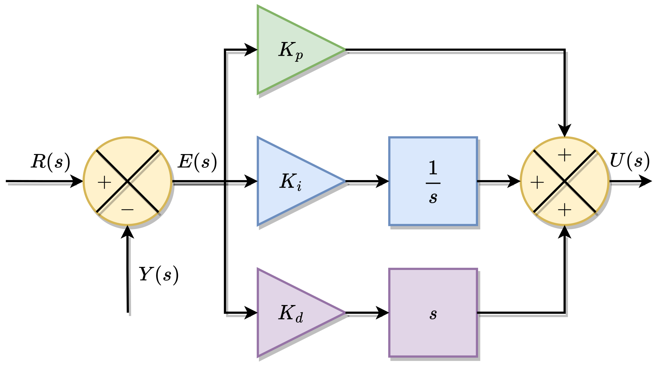
2.1. PID Controller
- Proportional Control: This term refers to correcting action proportionate to the present error.
- Integral Control: This term is a correction based on accumulating errors over time through low-frequency compensation.
- Derivative Control: This term applies a correction based on the error’s rate of change through high-frequency compensation.
2.2. PIDD Controller
2.3. FOPID Controller
2.4. Proposed PIDD Controller
3. Simulation Study
3.1. First-Order System
3.2. Second-Order Model with Inertia and Time Delay
3.3. Magnetic Levitation System
3.4. Automatic Voltage Regulation System
4. Experimental Study
4.1. Real-Time Pressure Process Plant
4.2. Real-Time Flow Process Plant
5. Conclusions
Author Contributions
Funding
Institutional Review Board Statement
Informed Consent Statement
Data Availability Statement
Conflicts of Interest
Abbreviations
| ABC | Artificial Bee Colony |
| AEF | Artificial Electric Field |
| ASO | Atom Search Optimization |
| AVR | Automatic Voltage Regulator |
| DOF | Degree of Freedom |
| FLC | Fuzzy Logic Control |
| FOPID | Fractional-order Proportional Integral Derivative |
| FPID | Fuzzy PID |
| FPIDD | Fuzzy Proportional-Integral-Derivative-Double Derivative |
| GA | Genetic Algorithm |
| GBO | Gradient-Based Optimization |
| IAE | Integral Absolute Error |
| IMC | Internal Model Control |
| ISAE | Integral Square Absolute Error |
| ISE | Integral Square Error |
| ITAE | Integral Time Absolute Error |
| ITSE | Integral Time Square Error |
| MAPE | Mean Absolute Percentage Error |
| MICE | Marine Internal Combustion Engines |
| P&ID | Piping and Instrumentation Diagram |
| PCI | Peripheral Interface Cards |
| PCV | Process Control Valve |
| PI | Proportional Integral |
| PID | Proportional Integral Derivative |
| PIDA | Proportional-Integral-Derivative-Acceleration |
| PIDD2 | PID with Derivative Filter |
| PSO | Particle Swarm Optimization |
| PT | Pressure Transmitter |
| RMSE | Root Mean Square Error |
| SCA | Sine Cosine Algorithm |
| WDO | Wind-Driven Optimization |
References
- Veinović, S.; Stojić, D.; Ivanović, L. Optimized PIDD2 controller for AVR systems regarding robustness. Int. J. Electr. Power Energy Syst. 2023, 145, 108646. [Google Scholar] [CrossRef]
- Jahanshahi, H.; Sari, N.N.; Pham, V.T.; Alsaadi, F.E.; Hayat, T. Optimal adaptive higher order controllers subject to sliding modes for a carrier system. Int. J. Adv. Robot. Syst. 2018, 15, 1729881418782097. [Google Scholar] [CrossRef]
- Chatterjee, S.; Mukherjee, V. Comparative performance analysis of classical controllers for automatic voltage regulator. In Proceedings of the 2017 7th International Conference on Power Systems (ICPS), Pune, India, 21–23 December 2017; pp. 296–301. [Google Scholar]
- Simanenkov, A.; Rozhkov, S.; Borisova, V. An algorithm of optimal settings for PIDD 2 D 3-controllers in ship power plant. In Proceedings of the 2017 IEEE 37th International Conference on Electronics and Nanotechnology (ELNANO), Kyiv, Ukraine, 18–20 April 2017; pp. 152–155. [Google Scholar]
- Devan, P.A.M.; Ibrahim, R.; Omar, M.B.; Bingi, K.; Abdulrab, H.; Hussin, F.A. Improved Whale Optimization Algorithm for Optimal Network Coverage in Industrial Wireless Sensor Networks. In Proceedings of the 2022 International Conference on Future Trends in Smart Communities (ICFTSC), Kuching, Malaysia, 1–2 December 2022; pp. 124–129. [Google Scholar]
- AboRas, K.M.; Ragab, M.; Shouran, M.; Alghamdi, S.; Kotb, H. Voltage and frequency regulation in smart grids via a unique Fuzzy PIDD2 controller optimized by Gradient-Based Optimization algorithm. Energy Rep. 2023, 9, 1201–1235. [Google Scholar] [CrossRef]
- Izci, D.; Ekinci, S.; Çetin, H. Arithmetic Optimization Algorithm based Controller Design for Automatic Voltage Regulator System. In Proceedings of the 2022 Innovations in Intelligent Systems and Applications Conference (ASYU), Antalya, Turkey, 7–9 September 2022; pp. 1–5. [Google Scholar]
- Devan, P.A.M.; Ibrahim, R.; Omar, M.; Bingi, K.; Abdulrab, H. A Novel Hybrid Harris Hawk-Arithmetic Optimization Algorithm for Industrial Wireless Mesh Networks. Sensors 2023, 23, 6224. [Google Scholar] [CrossRef]
- Izci, D.; Ekinci, S. An improved RUN optimizer based real PID plus second-order derivative controller design as a novel method to enhance transient response and robustness of an automatic voltage regulator. e-Prime-Adv. Electr. Eng. Electron. Energy 2022, 2, 100071. [Google Scholar] [CrossRef]
- Emiroglu, S.; Gümüş, T.E. Optimal Control of Automatic Voltage Regulator System with Coronavirus Herd Immunity Optimizer Algorithm-Based PID plus Second Order Derivative Controller. Acad. Platf. J. Eng. Smart Syst. 2022, 10, 174–183. [Google Scholar] [CrossRef]
- Omar, M.B.; Bingi, K.; Prusty, B.R.; Ibrahim, R. Recent advances and applications of spiral dynamics optimization algorithm: A review. Fractal Fract. 2022, 6, 27. [Google Scholar] [CrossRef]
- Agwa, A.; Elsayed, S.; Ahmed, M. Design of Optimal Controllers for Automatic Voltage Regulation Using Archimedes Optimizer. Intell. Autom. Soft Comput. 2022, 31, 799–815. [Google Scholar] [CrossRef]
- Micev, M.; Ćalasan, M.; Radulović, M. Optimal design of real PID plus second-order derivative controller for AVR system. In Proceedings of the 2021 25th International Conference on Information Technology (IT), Zabljak, Montenegro, 16–20 February 2021; pp. 1–4. [Google Scholar]
- Ćalasan, M.; Micev, M.; Radulović, M.; Zobaa, A.F.; Hasanien, H.M.; Abdel Aleem, S.H. Optimal PID controllers for avr system considering excitation voltage limitations using hybrid equilibrium optimizer. Machines 2021, 9, 265. [Google Scholar] [CrossRef]
- Micev, M.; Ćalasan, M.; Ali, Z.M.; Hasanien, H.M.; Aleem, S.H.A. Optimal design of automatic voltage regulation controller using hybrid simulated annealing–Manta ray foraging optimization algorithm. Ain Shams Eng. J. 2021, 12, 641–657. [Google Scholar] [CrossRef]
- Chatterjee, S.; Dalel, M.A.; Palavalasa, M. Design of PID plus second order derivative controller for automatic voltage regulator using whale optimizatio algorithm. In Proceedings of the 2019 3rd International Conference on Recent Developments in Control, Automation & Power Engineering (RDCAPE), Noida, India, 10–11 October 2019; pp. 574–579. [Google Scholar]
- Sahib, M.A. A novel optimal PID plus second order derivative controller for AVR system. Eng. Sci. Technol. Int. J. 2015, 18, 194–206. [Google Scholar] [CrossRef]
- Moschos, I.; Parisses, C. A novel optimal PIλDND2N2 controller using coyote optimization algorithm for an AVR system. Eng. Sci. Technol. Int. J. 2022, 26, 100991. [Google Scholar] [CrossRef]
- Tabak, A. A novel fractional order PID plus derivative (PIλDμDμ2) controller for AVR system using equilibrium optimizer. COMPEL Int. J. Comput. Math. Electr. Electron. Eng. 2021, 40, 722–743. [Google Scholar] [CrossRef]
- Hossam-Eldin, A.A.; Negm, E.; Ragab, M.; AboRas, K.M. A maiden robust FPIDD2 regulator for frequency-voltage enhancement in a hybrid interconnected power system using Gradient-Based Optimizer. Alexandria Eng. J. 2023, 65, 103–118. [Google Scholar] [CrossRef]
- Priyadarshani, S.; Satapathy, J. Novel Application of Gradient-Based Optimizer for tuning a Fuzzy-PIDD 2 controller for Load Frequency Stabilization. In Proceedings of the 2021 IEEE International Conference on Electronics, Computing and Communication Technologies (CONECCT), Bangalore, India, 8–10 July 2022; pp. 1–6. [Google Scholar]
- Khudhair, M.; Ragab, M.; AboRas, K.M.; Abbasy, N.H. Robust control of frequency variations for a multi-area power system in smart grid using a newly wild horse optimized combination of PIDD2 and PD controllers. Sustainability 2022, 14, 8223. [Google Scholar] [CrossRef]
- Kumar, M.; Hote, Y.V. Robust PIDD2 controller design for perturbed load frequency control of an interconnected time-delayed power systems. IEEE Trans. Control Syst. Technol. 2020, 29, 2662–2669. [Google Scholar] [CrossRef]
- Shankar, R. Sine-Cosine algorithm based PIDD 2 controller design for AGC of a multisource power system incorporating GTPP in DG unit. In Proceedings of the 2018 International Conference on Computational and Characterization Techniques in Engineering & Sciences (CCTES), Lucknow, India, 14–15 September 2018; pp. 197–201. [Google Scholar]
- Debbarma, S.; Nath, A.; Sarma, U.; Saikia, L.C. Cuckoo search algorithm based two degree of freedom controller for multi-area thermal system. In Proceedings of the 2015 International Conference on Energy, Power and Environment: Towards Sustainable Growth (ICEPE), Shillong, India, 12–13 June 2015; pp. 1–6. [Google Scholar]
- Lazarević, M.P.; Mandić, P.D.; Cvetković, B.; Bučanović, L.; Dragović, M. Advanced open-closed-loop PIDD 2/PID type ILC control of a robot arm. In Proceedings of the 2018 Innovations in Intelligent Systems and Applications (INISTA), Thessaloniki, Greece, 3–5 July 2018; pp. 1–8. [Google Scholar]
- Todd, C.; Koujan, H.; Fasciani, S. A Hybrid Controller for Inflight Stability and Maneuverability of an Unmanned Aerial Vehicle in Indoor Terrains. Autom. Control Syst. Eng. J. 2017, 17, 27–39. [Google Scholar]
- Izci, D.; Ekinci, S.; Eker, E.; Dündar, A. Assessment of slime mould algorithm based real PID plus second-order derivative controller for magnetic levitation system. In Proceedings of the 2021 5th International Symposium on Multidisciplinary Studies and Innovative Technologies (ISMSIT), Ankara, Turkey, 21–23 October 2021; pp. 6–10. [Google Scholar]
- Simanenkov, A. An analysis of PIDD2 controllers optimal adjusting algorithm in mpp fuel preparation system. EUREKA Phys. Eng. 2017, 3–12. [Google Scholar] [CrossRef]
- Qiankun, M.; Xuyong, W.; Fan, Y.; Jianfeng, T.; Peng, L. Research on feed-forward PIDD2 control for hydraulic continuous rotation motor electro-hydraulic servo system with long pipeline. In Proceedings of the 2016 UKACC 11th International Conference on Control (CONTROL), Belfast, UK, 31 August–2 September 2016; pp. 1–6. [Google Scholar]
- Zhou, K.; Wang, X.; Tao, J.; Guo, X.; Xu, C. Research on a novel PID based controller for nonmagnetic hydraulic navigation simulator with AMESim simulation. In Proceedings of the 2012 UKACC International Conference on Control, Cardiff, UK, 3–5 September 2012; pp. 496–501. [Google Scholar]
- Pashchenko, F.; Pikina, G.; Rodomanova, Y. Universal searchless method for parametric optimization of predictive algorithms. In Proceedings of the 2017 13th IEEE International Conference on Control & Automation (ICCA), Ohrid, North Macedonia, 3–6 July 2017; pp. 952–957. [Google Scholar]
- Izvoreanu, B.; Cojuhari, I. The Tuning of the PID and PIDD2 Algorithms to the Model Objects with Inertia and Identical Elements and Time Delay. 2013. Available online: http://repository.utm.md/handle/5014/17375 (accessed on 15 July 2023).
- Alexík, M. Adaptive Self-Tuning PIDD2 Algorithm. IFAC Proc. Vol. 2003, 36, 83–88. [Google Scholar] [CrossRef]
- Huba, M. Extending spectrum of filtered controllers for ipdt plant models. In Proceedings of the 2018 Cybernetics & Informatics (K&I), Lazy pod Makytou, Slovakia, 31 January–3 February 2018; pp. 1–6. [Google Scholar]
- Jaradat, M.A.; Sawaqed, L.S.; Alzgool, M.M. Optimization of PIDD2-FLC for blood glucose level using particle swarm optimization with linearly decreasing weight. Biomed. Signal Process. Control 2020, 59, 101922. [Google Scholar] [CrossRef]
- Kumar, M.; Hote, Y.V. PIDD2 Controller Design Based on Internal Model Control Approach for a Non-Ideal DC-DC Boost Converter. In Proceedings of the 2021 IEEE Texas Power and Energy Conference (TPEC), College Station, TX, USA, 2–5 February 2021; pp. 1–6. [Google Scholar]
- Bingi, K.; Ibrahim, R.; Karsiti, M.N.; Hassan, S.M.; Harindran, V.R. Fractional-Order Systems and PID Controllers; Springer: Berlin/Heidelberg, Germany, 2020; Volume 264. [Google Scholar]
- Mystkowski, A.; Zolotas, A. PLC-based discrete fractional-order control design for an industrial-oriented water tank volume system with input delay. Fract. Calc. Appl. Anal. 2018, 21, 1005–1026. [Google Scholar] [CrossRef]
- Lendek, A.; Tan, L. Mitigation of derivative kick using time-varying fractional-order PID control. IEEE Access 2021, 9, 55974–55987. [Google Scholar] [CrossRef]
- Ghamari, S.M.; Narm, H.G.; Mollaee, H. Fractional-order fuzzy PID controller design on buck converter with antlion optimization algorithm. IET Control Theory Appl. 2022, 16, 340–352. [Google Scholar] [CrossRef]
- Bingi, K.; Ibrahim, R.; Karsiti, M.N.; Hassan, S.M. Fractional order set-point weighted PID controller for pH neutralization process using accelerated PSO algorithm. Arab. J. Sci. Eng. 2018, 43, 2687–2701. [Google Scholar] [CrossRef]
- Bingi, K.; Ibrahim, R.; Karsiti, M.N.; Hassam, S.M.; Harindran, V.R. Frequency response based curve fitting approximation of fractional-order PID controllers. Int. J. Appl. Math. Comput. Sci. 2019, 29, 311–326. [Google Scholar] [CrossRef]
- Faieghi, M.R.; Nemati, A. On fractional-order PID design. In Applications of MATLAB in Science and Engineering; IntechOpen: London, UK, 2011. [Google Scholar]
- Shanmugam, S.K.; Duraisamy, Y.; Ramachandran, M.; Arumugam, S. Mathematical modeling of first order process with dead time using various tuning methods for industrial applications. Math. Model. Eng. 2019, 5, 1–10. [Google Scholar] [CrossRef]
- Bingi, K.; Rajanarayan Prusty, B.; Pal Singh, A. A Review on Fractional-Order Modelling and Control of Robotic Manipulators. Fractal Fract. 2023, 7, 77. [Google Scholar] [CrossRef]


| Ref. | Year | Controller | Parameters | Comparison | System | Tuning | Measures | Simulation/Practical | Software |
|---|---|---|---|---|---|---|---|---|---|
| [6] | 2023 | Fuzzy PIDD | 8 | PID, Fuzzy PID | Conventional and hybrid two-area power systems | Gradient-based optimization | ITAE | Simulation | MATLAB |
| [1] | 2023 | PIDD | 5 | PID | AVR of synchronous generator | Constrained optimization problem via an iterative procedure | IAE | Practical | MATLAB |
| [20] | 2023 | FPIDD | 6 | GBO tuned ID-T, FPID | Two-area hybrid system | Gradient-based optimisation | rise time, settling time, max overshoot and undershoot, ITAE | Simulation and Practical | MATLAB/Simulink |
| [22] | 2022 | PIDD-PD | 9 | PID-TID, ID-T | Two-area linked power system | Wild horse optimizer | Settling time, maximum overshoot, and undershoot values | Simulation | MATLAB/Simulink |
| [10] | 2022 | PIDD | 4 | IWO-PIDD, PSO-PIDD, OBASO-PIDD, ASO-PIDD | AVR system | Coronavirus herd immunity optimization | ITAE, ITSE | Simulation and Practical | MATLAB |
| [7] | 2022 | PIDD-PD | 6 | PIDD-PSO, FOPID-SMA, PID-SCA, PIDA-WOA | AVR system | Arithmetic optimisation algorithm | overshoot, rise time, settling time, phase margin, bandwidth | Simulation | MATLAB |
| [9] | 2022 | PIDD | 6 | PID, PID-F, PIDA, FOPID, PIDD | AVR system | Improved Runge Kutta optimiser | rise time, settling time, percent overshoot | Simulation | – |
| [12] | 2022 | PIDD | 4 | PID, FOPID, RPID, SPID | AVR system | Archimedes optimization algorithm | settling time, rise time, overshoot voltage | Simulation | – |
| [18] | 2022 | PIkDND2N2 | 7 | FOPID, PID, PIDA, PIDD | AVR system | Coyote optimization algorithm | transient response and disturbance rejection | Simulation | MATLAB |
| [37] | 2021 | PIDD | 4 | IMC PID | Non-ideal DC-DC boost converter | Internal model control | max sensitivity, rise time, total variation | Practical | MATLAB |
| [13] | 2021 | PIDD | 6 | PID, FOPID, ideal PIDD | AVR system | Equilibrium optimizer | rise time, settling time, overshoot | Simulation | – |
| [14] | 2021 | PIDD | 4 | SA-MRFO-PIDD, PSO-PIDD, AEO-PID | AVR system | Equilibrium optimizer-evaporation rate water cycle | rise time, delay time, overshoot | Simulation | MATLAB |
| [21] | 2021 | Fuzzy PIDD | 5 | (HSCOA, GBO, BFO)-FPIDD, FPID, PID | Two-area linear thermal model and linear multi-source topology in two-area environments | Gradient-based optimisation | settling time, maximum overshoot, and undershoot values | Simulation | MATLAB/Simulink |
| [28] | 2021 | PIDD-PID | 6 | (ASO, AEF, ABC)-FOPID, (SCA, WDO, ABC)-ideal PID | Magnetic levitation system | Slime mould algorithm | settling time, rise time, overshoot voltage | Simulation | MATLAB |
| [19] | 2021 | FOPIDD | 7 | FOPID, PID, PIDA, PIDD | AVR system | Equilibrium Optimizer | settling time, rise time, overshoot voltage | Simulation | MATLAB |
| [23] | 2021 | PIDD | 4 | PI, PID | Two-area time delayed power system model | Internal model control | Settling time, maximum overshoot and undershoot values | Simulation | MATLAB/Simulink |
| [15] | 2021 | PIDD | 5 | ideal PID, real PID, FOPID, PIDD | AVR system | Simulated annealing—Manta ray foraging optimization algorithm | settling time, rise time, overshoot voltage | Simulation | MATLAB |
| [36] | 2020 | Fuzzy PIDD | 9 | PD, PI, parallel PID, and single-rule-based PID fuzzy controllers | Two-delay differential model | Particle swarm optimization with linearly decreasing weight | MAPE, RMSE, insulin used | Simulation | – |
| [16] | 2019 | PIDD | 4 | (MOL, PSO, CS, ABC)-PID | AVR system | Whale optimisation algorithm | settling time, rise time, overshoot voltage | Simulation | MATLAB/Simulink |
| [24] | 2018 | PIDD | 7 | – | Two-area power system | Sine cosine algorithm | ISE | Simulation | MATLAB/Simulink |
| [35] | 2018 | PIDD | 4 | PI, PID, PIDD | IPDT plant model | Quintuple real dominant poles tuning | IAE | Simulation | MATLAB/Simulink |
| [26] | 2018 | PIDD/PID | 8 | – | Neuroarm robotic manipulator | Iterative learning control | – | Simulation and Practical | – |
| [2] | 2018 | PI2IDD2, PI2ID, PIDD, PID2, and PI2D | 3 to 5 | PI2IDD2, PI2ID, PIDD, PID2, and PI2D | Cansat carrier launch system | Multi-objective GA | time response of angular velocity and control gain | Practical | – |
| [32] | 2017 | PIDD | 4 | predictive PID | 3rd-order model with time delay | Universal search-less method | transient response of set-point signal | Simulation | – |
| [3] | 2017 | PIDD | 4 | PID tuned with DEA, PSO, ABC algorithms and LQR method | AVR system | Linear quadratic method | peak magnitude, rise time, settling time | Simulation | MATLAB |
| [4] | 2017 | PIDDD3 | 5 | PID, PIDD | Ship power plant | Simulation model of a digital control system | integral index, oscillation index | Simulation | MATLAB |
| [29] | 2017 | PIDD | 4 | PID | MICE fuel preparation system | – | integral criterion, oscillation index, control parameter deviation | Simulation | MATLAB |
| [27] | 2017 | FLC-PID-PIDD | 4 | FLC PID, PID | Unmanned aerial vehicles in indoor terrains | Complimentary error minimization algorithms | response time, control accuracy | Simulation | MATLAB/Simulink |
| [30] | 2016 | Feedforward PIDD | 4 | PID | Hydraulic continuous rotation motor electro-hydraulic servo system | – | system response | Simulation | AMESim |
| [25] | 2015 | 2-DOF-PIDD | 6 | I, PI, PID | Multi-area thermal system | Cuckoo search algorithm | settling time, peak overshoot, oscillation rate | Simulation | MATLAB |
| [17] | 2015 | PIDD | 4 | PID, FOPID with other tuning algorithms | AVR system | Particle swarm optimization | maximum overshoot, rise time, settling time | Simulation | MATLAB |
| [33] | 2013 | PIDD | 4 | PID | 2nd-order model with inertia and time delay | Maximal stability degree method with iteration | control time, overshoot | Simulation | MATLAB |
| [31] | 2012 | Feedforward PIDD | 4 | PID, PIDD, Dff-PID | Valve-controlled hydraulic motor system | – | position tracking capability | Simulation | AMESim |
| [34] | 2003 | PIDD | 4 | PID | Analogue model of control plant | Identification algorithm REDIC | transient responses | Simulation and Practical | ADAPTLAB |
| Controller | ||||||||||
|---|---|---|---|---|---|---|---|---|---|---|
| PID | 1 | 1 | 2 | – | - | – | – | 20.3731 | 3.6417 | 27.4682 |
| PIDD | 1 | 1 | 2 | 1 | - | – | – | 22.8111 | 4.985 | 28.1916 |
| FOPID | 1 | 1 | 2 | – | 0.5 | 0.98 | – | 9.6332 | 3.8846 | 14.2615 |
| PIDD | 1 | 1 | 2 | 1 | – | – | 0.1 | 11.068 | 3.867 | 14.2194 |
| Controller | ||||||||||
|---|---|---|---|---|---|---|---|---|---|---|
| PID | 17.5 | 4.12 | 9.46 | – | – | – | – | 3.7692 | 0.3821 | 6.1165 |
| PIDD | 17.5 | 4.12 | 9.46 | 0.3 | – | – | – | 0 | 0.4606 | 6.1126 |
| FOPID | 17.5 | 4.12 | 9.46 | – | 1 | 1.2 | – | 2.9108 | 0.3869 | 3.1772 |
| PIDD | 17.5 | 4.12 | 9.46 | 0.3 | – | – | 1.75 | 0.0864 | 0.4037 | 6.1118 |
| Controller | ||||||||||
|---|---|---|---|---|---|---|---|---|---|---|
| PID | −159 | −139 | −8 | – | – | – | – | 44.5024 | 0.0167 | 0.1723 |
| PIDD | −159 | −139 | −8 | −0.18 | – | – | – | 13.0223 | 0.0207 | 0.1914 |
| FOPID | −159 | −139 | −8 | – | 0.9 | 1.1 | – | 35.1198 | 0.0128 | 0.1989 |
| PIDD | −159 | −139 | −8 | −0.18 | – | – | 2.04 | 12.8299 | 0.0075 | 0.2025 |
| Controller | ||||||||||
|---|---|---|---|---|---|---|---|---|---|---|
| PID | 4.8938 | 3.2301 | 2.2479 | - | - | - | - | 4.7876 | 0.2582 | 1.1458 |
| PIDD | 4.8938 | 3.2301 | 2.2479 | 0.2048 | - | - | - | 0.2872 | 0.0245 | 0.0373 |
| FOPID | 4.8938 | 3.2301 | 2.2479 | - | 1.1122 | 1.0624 | - | 3.8758 | 0.2196 | 0.9012 |
| PIDD | 4.8938 | 3.2301 | 2.2479 | 0.2048 | – | – | 2.01 | 0.1923 | 0.0232 | 0.0984 |
| Controller | ||||||||||
|---|---|---|---|---|---|---|---|---|---|---|
| PID | 0.5 | 0.5 | −0.01 | - | - | - | - | 6.2148 | 2.8287 | 9.2664 |
| PIDD | 0.5 | 0.5 | −0.01 | −0.1 | - | - | - | 5.1179 | 2.8486 | 9.0571 |
| FOPID | 0.5 | 0.5 | −0.01 | - | 0.99 | 0.15 | - | 5.5126 | 2.8792 | 8.96 |
| PIDD | 0.5 | 0.5 | −0.01 | −0.1 | - | - | 1.7 | 4.838 | 2.6272 | 8.9543 |
| Controller | ||||||||||
|---|---|---|---|---|---|---|---|---|---|---|
| PID | 1 | 1 | 0.1 | - | - | - | - | 0 | 25.8559 | 46.788 |
| PIDD | 1 | 1 | 0.1 | −0.01 | - | - | - | 0 | 25.8284 | 46.2981 |
| FOPID | 1 | 1 | 0.1 | - | 0.99 | 0.1 | - | 0 | 27.2797 | 50.6053 |
| PIDD | 1 | 1 | 0.1 | −0.01 | - | - | 2.05 | 0 | 25.7819 | 46.0495 |
Disclaimer/Publisher’s Note: The statements, opinions and data contained in all publications are solely those of the individual author(s) and contributor(s) and not of MDPI and/or the editor(s). MDPI and/or the editor(s) disclaim responsibility for any injury to people or property resulting from any ideas, methods, instructions or products referred to in the content. |
© 2023 by the authors. Licensee MDPI, Basel, Switzerland. This article is an open access article distributed under the terms and conditions of the Creative Commons Attribution (CC BY) license (https://creativecommons.org/licenses/by/4.0/).
Share and Cite
Fawwaz, M.A.; Bingi, K.; Ibrahim, R.; Devan, P.A.M.; Prusty, B.R. Design of PIDDα Controller for Robust Performance of Process Plants. Algorithms 2023, 16, 437. https://doi.org/10.3390/a16090437
Fawwaz MA, Bingi K, Ibrahim R, Devan PAM, Prusty BR. Design of PIDDα Controller for Robust Performance of Process Plants. Algorithms. 2023; 16(9):437. https://doi.org/10.3390/a16090437
Chicago/Turabian StyleFawwaz, Muhammad Amir, Kishore Bingi, Rosdiazli Ibrahim, P. Arun Mozhi Devan, and B. Rajanarayan Prusty. 2023. "Design of PIDDα Controller for Robust Performance of Process Plants" Algorithms 16, no. 9: 437. https://doi.org/10.3390/a16090437
APA StyleFawwaz, M. A., Bingi, K., Ibrahim, R., Devan, P. A. M., & Prusty, B. R. (2023). Design of PIDDα Controller for Robust Performance of Process Plants. Algorithms, 16(9), 437. https://doi.org/10.3390/a16090437